Reconciling Semiclassical and Bohmian Mechanics:
III. Scattering states for continuous potentials

Abstract

In a previous paper [J. Chem. Phys. 121 4501 (2004)] a unique bipolar decomposition, $\Psi=\Psi_{1}+\Psi_{2}$ was presented for stationary bound states $\Psi$ of the one-dimensional Schrödinger equation, such that the components $\Psi_{1}$ and $\Psi_{2}$ approach their semiclassical WKB analogs in the large action limit. The corresponding bipolar quantum trajectories, as defined in the usual Bohmian mechanical formulation, are classical-like and well-behaved, even when $\Psi$ has many nodes, or is wildly oscillatory. A modification for discontinuous potential stationary stattering states was presented in a second paper [J. Chem. Phys. !!! !!!! (2005)], whose generalization for continuous potentials is given here. The result is an exact quantum scattering methodology using classical trajectories. For additional convenience in handling the tunneling case, a constant velocity trajectory version is also developed.

I INTRODUCTION

This paper is the third in a series investigating the use of “counter-propagating wave methods” (CPWMs)poirier04bohmI ; poirier05bohmII ; babyuk04 ; wyatt for solving the Schrödinger equation exactly. CPWMs are a particular variant of the more general multipolar decomposition methods, wherein the wavefunction $\Psi$ is decomposed into two or more components, $\Psi_{j}$. Thus, for a two-term, or “bipolar” decomposition, $\Psi=\Psi_{1}+\Psi_{2}$. This rather trivial-seeming procedure can be quite advantageous in the context of quantum trajectory methods (QTMs),wyatt ; lopreore99 ; mayor99 ; wyatt99 ; shalashilin00 ; wyatt01b ; wyatt01c ; burghardt01b ; bittner02b ; hughes03 i.e. trajectory-based numerical techniques for performing exact quantum dynamics calculations, based on Bohmian mechanics.madelung26 ; vanvleck28 ; bohm52a ; bohm52b ; takabayasi54 ; holland Conventional QTMs use a single-term or “unipolar” representation of the wavefunction from which all other quantities, such as the quantum trajectories themselves, are uniquely determined. Multipolar decomposition, on the other hand, can lead to radically different QTM behavior for the individual $\Psi_{j}$ components, owing to the fact that the Bohmian equations of motion are non-linear.poirier04bohmI ; poirier05bohmII

As applied to wavepacket dynamics for reactive scattering systems, QTMs suffer from a significant and well-known numerical drawback, which to date, precludes a completely robust application of these methods. Namely, QTMs are numerically unstable in the vicinity of amplitude nodes and “quasi-nodes” (i.e. rapid oscillations),wyatt ; wyatt01b owing to singularities in the “quantum potential,” $Q$, which together with the classical potential, $V$, determines the quantum trajectories. In the reactive scattering context, such behavior is always observed, due to interference between the incident and reflected waves. On the other hand, if the latter two contributions to the total $\Psi$ were somehow separated, and associated with two different interference-free $\Psi_{j}$ components, the node problem might well be circumvented. If, in addition, the $\Psi_{j}$ component field functions were smooth and slowly-varying, far fewer QTM trajectories and time-steps might be required than for $\Psi$ itself—although the latter could be reconstructed at any desired time simply via linear superposition of the components. These numerical advantages thus provide significant motivation for consideration of the bipolar approach. A much more detailed discussion may be found in the first two articles of this series, paper I (LABEL:poirier04bohmI) and paper II (LABEL:poirier05bohmII).

The most obvious aspect of any bipolar decomposition, including those restricted along the lines of the preceding paragraph,poirier04bohmI ; poirier05bohmII ; floyd94 ; brown02 is that it is not unique. The covering function method,babyuk04 ; wyatt for instance, treats $\Psi$ as the difference between two very large-amplitude components, thus “diluting” the effects of interference. The one-dimensional (1D) CPWM approach,poirier04bohmI ; poirier05bohmII on the other hand, regards the bipolar decomposition

$$\Psi=\Psi_{+}+\Psi_{-}$$ (1)

as a superposition of right- and left-traveling counter-propagating waves, $\Psi_{\pm}$. For stationary states at least, the Eq. (1) decomposition is defined such that the $\Psi_{\pm}$ components correspond to semiclassical WKB approximations, $\Psi_{\pm}^{\text{sc}}$, in the large-action limit. In addition to providing pedagogical value (semiclassical and Bohmian mechanics can not be so reconciled in a unipolar context), the semiclassical field functions are typically smooth and slowly-varying, i.e. the semiclassical-like CPWM components $\Psi_{\pm}$ provide the desirable numerical advantages described in the preceding paragraph.

In paper I (LABEL:poirier04bohmI), a unique CPWM bipolar decomposition was determined for bound stationary eigenstates of arbitrary 1D Hamiltonians. The resultant $\Psi_{\pm}$ field functions are smooth and interference-free, and approach the WKB approximations in the large-action limit (within the classically allowed region of space) as desired. Moreover, the quantum potentials $q_{\pm}$ become vanishingly small in this limit, so that the bipolar quantum trajectories approach classical trajectories, and only a small number are required for a numerical propagation, regardless of excitation energy, $E$. In contrast, the unipolar $\Psi$ exhibits motionless trajectories, and an arbitrarily increasing number of nodes in the large-action/energy limit. Results were presented for both the harmonic and Morse oscillator potentials.

In paper II (LABEL:poirier05bohmII), the 1D CPWM ideas were modified somewhat for stationary scattering states of discontinuous potentials. Although the CPWM decomposition of paper I is uniquely specified for any arbitrary 1D eigenstate—bound or scattering—and in the bound case, always satisfies the correspondence principle, the non-$L^{2}$ nature of the scattering states is such that the paper I decomposition generally does not satisfy correspondence globally. As discussed in Sec. II.1, this requires that global modifications must be made in order to enable a correspondence between $\Psi_{\pm}^{\text{sc}}$ and $\Psi_{\pm}$. These are such as to lead to substantial differences between the density functions $|\Psi_{\pm}^{\text{sc}}(x)|^{2}$ and $|\Psi_{\pm}(x)|^{2}$, although the trajectories are identical. Moreover, the resultant $\Psi_{\pm}$ are found to correspond to the familiar “incident,” “transmitted,” and “reflected” waves of traditional scattering theorytaylor in the appropriate asymptotic limits. From the time-dependent standpoint, reflection was found to be due to trajectory hopping from one CPWM component to the other, as can be naturally understood using a simple ray optics analogy. The method was applied to several elementary discontinuous potential systems, including the square barrier/well.

In the present paper (paper III), the LABEL:poirier05bohmII formulations are generalized to incorporate both continuous and discontinuous potential systems. Once again, an analogy is drawn from semiclassical mechanics, albeit a “sophisticated” versionheading ; froman ; berry72 less frequently considered (Sec. II.1). As in paper II, a time-dependent method based on ray optics is developed for computing stationary states of any desired energy and boundary conditions. For the most part, the discussion of the preceding paragraph still applies, but some additional key points should be emphasized. First, the bipolar decomposition now provides a sensible definition of “incident,” “transmitted,” and “reflected” waves throughout all space, not just asymptotically. Second, the explicit hopping of trajectories from one CPWM component to the other is replaced with a coupling term in the time-evolution equations. Third, the trajectories become completely classical. Finally, an alternative methodology is also developed, based on the use of constant velocity trajectories, which can be readily applied to barrier tunneling situations. The new methods are found to be remarkably efficient, accurate, and robust across a diverse range of 1D test potentials and system energies (Sec. IV).

The paper is organized as follows. A derivation and discussion of the time-evolution equations for the CPWM bipolar components $\Psi_{\pm}$, both for classical and constant velocity trajectories, are presented in Sec. II and the Appendices. Sec. III provides numerical details of the various bipolar algorithms used to compute stationary states. Results are presented in Sec. IV for four benchmark applications: Eckart barrier; square barrier; uphill ramp; double-Gaussian barrier. For the first three, these are compared with known analytic solutions. Concluding remarks, including prospects for future development, may be found in Sec. V.

II THEORY

II.1 Semiclassical Approximations

Let $V(x)$ be the potential energy for a 1D scattering system, and $E$ the energy of some stationary state $\Psi(x)$ such that $E>V(x)$ for all $x$. In reality, $\Psi(x)$ always manifests some reflection, even though the energy is above the potential barrier. However, basic WKB theory predicts zero reflection in this case, as the classical trajectories do not turn around. This is also evident from the form of the two basic WKB counter-propagating wave solutions,

$$\Psi_{\pm}^{\text{sc}}(x)=r_{\text{sc}}(x)e^{\pm is_{\text{sc}}(x)/\hbar},$$ (2)

where

$$r_{\text{sc}}(x)=\sqrt{{mF\over s^{\prime}_{\text{sc}}(x)}}\quad\text{and}\quad s^{\prime}_{\text{sc}}(x)=\sqrt{2m\left[{E-V(x)}\right]},$$ (3)

$m$ is the mass, $F$ is the invariant flux (paper I), and primes denote spatial differentiation. Note that since scattering solutions are non-square-integrable, the choice of $F$ is arbitrary; however, throughout this paper we shall adopt the usual left-incident wave normalization convention, $\lim_{x\rightarrow-\infty}r_{\text{sc}}(x)=1$, so that $F=\lim_{x\rightarrow-\infty}s^{\prime}_{\text{sc}}(x)/m$. The positive and negative momentum functions, $p_{\pm}^{\text{sc}}(x)=\pm s^{\prime}_{\text{sc}}(x)$, specify the classical trajectories and semiclassical Lagrangian manifoldspoirier04bohmI ; keller60 ; maslov ; littlejohn92 (LMs) associated with the $\Psi_{\pm}^{\text{sc}}(x)$ solutions. Clearly, the classical trajectories do not change direction, as there are no turning points along the real $x$ axis. Therefore, for an arbitrary linear combination solution,

$$\Psi=\alpha_{+}\Psi_{+}^{\text{sc}}+\alpha_{-}\Psi_{-}^{\text{sc}},$$ (4)

the entire reflected wave must be due to the $\Psi_{-}^{\text{sc}}(x)$ contribution. The boundary conditions presume that the left-traveling wave contribution vanish in the $x\rightarrow\infty$ limit, implying that $\alpha_{-}=0$ and $\Psi(x)=\Psi_{+}(x)$—i.e., there is no reflected wave.

Various strategies have been developed to deal with the above difficulty of the basic WKB method.heading ; froman ; berry72 The most common involve analytic continuation into the complex plane. Specifically, if no turning point is located along the real axis, then one is found elsewhere in the complex plane. The path of the incident wave is deformed so as to give rise to a reflected wave upon encountering the complex turning point. An analysis of the Stokes and anti-Stokes linesheading ; froman ; berry72 ; child ; poirier03capII that emanate from the complex turning point and cross the real $x$ axis, enables one to effectively recast the above procedure in terms of purely real-valued $x$. The net effect (as interpreted in this paper) is the introduction of coupling from $\Psi_{+}=\alpha_{+}\Psi_{+}^{\text{sc}}$ to $\Psi_{-}=\alpha_{-}\Psi_{-}^{\text{sc}}$, resulting in an $\alpha_{-}$ value that changes over $x$, thus yielding meaningful semiclassical partial reflection probabilities.

Alternatively, there is an approach due to Bremmerheading ; berry72 ; bremmer51 that from the start is formulated entirely on the real $x$ axis. This approach is preferred for the present purpose, as it provides a common bipolar foundation not only for basic WKB and “sophisticated” (i.e. capable of predicting partial reflection) semiclassical methods, but also for exact quantum scattering applications, as will be shown in Sec. II.2. Bremmer’s idea is to model the continuous potential $V(x)$ using a collection of discontinuous steps. Solutions are determined for an arbitrary step size, which is then made infinitesimally small.

Locally, along any given step, the two “exact” Schrödinger solutions (for the model step potential) are plane waves, $\exp(\pm ip_{k}x)$, where $p_{k}=\sqrt{2m\left(E-V_{k}\right)}$, and $V_{k}$ is the (constant) potential value along the $k$’th step (Appendix A). A viable global solution, $\Psi(x)$, must match boundary conditions appropriately at each of the step edges. In reality, a pure positive momentum local plane wave in one step would be joined to some linear combination of positive and negative momentum plane waves in the adjacent step, corresponding to partial reflection and transmission off of the local step. If the reflection contribution is ignored, e.g. so that only positive momentum local plane waves are involved, then the resultant approximate global solution can be easily shown to be just $\Psi_{+}^{\text{sc}}(x)$ in the limit of infinitesimal step size. Similarly, $\Psi_{-}^{\text{sc}}(x)$ is obtained from the negative momentum local plane waves. This approximation thus leads to the uncoupled basic WKB solutions of Eqs. (2) and (3).

The above approach clearly demonstrates how “continuous reflection”poirier03capI —i.e. that arising from continuous potentials—may be interpreted in more familiar discontinuous terms. It also suggests that reflection requires coupling between positive and negative momentum wavefunction components. This approach has been used to develop a sophisticated WKB approximation, similar to the Stokes/anti-Stokes approach described above, wherein one-way reflection from $\Psi_{+}$ to $\Psi_{-}$ is retained, but back reflection is ignored.berry72 On the other hand, if all reflection is retained, one can derive a coupled pair of first order differential equations for $\Psi_{\pm}$ that exactly describes the quantum scattering solution $\Psi$ of Eq. (1). Although the $\Psi_{\pm}$ components are not themselves stationary solutions, they do correspond to the familiar incident/transmitted/reflected interpretations as discussed in paper II.

II.2 Exact Quantum Dynamics Using Classical Trajectories

II.2.1 Time-evolution equations

In paper II, an exact quantum, CPWM bipolar decomposition scheme for stationary scattering states was presented such that a suitable $\Psi_{\pm}$ could be constructed for a solution $\Psi$ with any desired boundary conditions, using a simple time-dependent approach. The classical trajectories and LMs were found to be identical to those of the basic WKB approximations, $\Psi_{\pm}^{\text{sc}}(x)$—thus satisfying the correspondence principle, and giving rise to smooth, well-behaved, interference-free CPWM component functions, $\Psi_{\pm}$. Although the method formally applies only to discontinuous potentials, Sec. II.1 suggests that it ought to be extendible to continuous potentials as well, simply by modeling the latter using infinitesimally small steps. This idea is indeed quite straightforward to implement, as discussed in Appendix A and Fig. 1. As in paper II, the result is a trajectory-based scattering methodology that is both local and exact in its treatment of reflection and transmission, due to the time-dependent nature of the approach. In contrast, the global character of reflection and transmission in conventional time-independent exact quantum methods is well-recognized. Of the time-independent semiclassical approximations, the most sophisticated depend on the relative placement of local potential features such as discontinuities and turning points,heading ; froman ; berry72 although the more approximate methods treat such features independently.

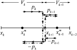
Figure 1: Time-dependent analysis of the $\Psi_{\pm}$ coupling, obtained via trajectory hopping due to local reflection off of infinitesimal potential steps. Continuous potential reflection is thus described in more pedagogical discontinuous terms.

From Appendix A, the hydrodynamic (Lagrangian) time-evolution equations for the CPWM bipolar components are found to be

$${d\Psi_{\pm}\over dt}=\left[{\mp{p^{\prime}\over 2m}+{i\over\hbar}\left(E-2V\right)}\right]\Psi_{\pm}\pm{p^{\prime}\over 2m}\Psi_{\mp},$$ (5)

where $\pm p=\pm\sqrt{2m(E-V)}$ are the momenta, which define the $\Psi_{\pm}$ LM and trajectories. Note that as expected, these are identical to those of $\Psi_{\pm}^{\text{sc}}(x)$, i.e. the trajectories are completely classical even though the solutions are exactly quantum mechanical (Appendix B). All of the other desirable properties, as described in the preceding paragraph and in paper II, are also found to be true.

II.2.2 Comparison with unipolar Bohmian mechanics

It is worthwhile to compare Eq. (5) with the usual unipolar evolution equations of Bohmian mechanics.wyatt ; bohm52a ; bohm52b ; holland Both are exact QTMs, but quantum effects are incorporated in very different ways. In unipolar Bohmian mechanics, the trajectory evolution is determined by the modified potential $V+Q$, where the quantum potential correction $Q$ is responsible for all quantum effects. Evaluation of $Q$ requires explicit double spatial differentiation of the wavefunction $\Psi$, which in turn requires specialized numerical techniques (Sec. III.2). Also, $Q$ diverges at nodes, and is otherwise numerically unstable in the presence of interference. In contrast, the present bipolar QTM scheme avoids interference difficulties as desired, owing to the semiclassical correspondence. Quantum effects do not manifest in the trajectories themselves (as these evolve completely classically), and there is no quantum potential in Eq. (5).

So where do quantum effects come from in Eq. (5)? As anticipated in Sec. II.1, these must be due to inter-component coupling, i.e. the last term in the equation. Note that the amount of coupling is proportional to $p^{\prime}\propto V^{\prime}$. Thus, the coupling vanishes in the limit that $V^{\prime}\rightarrow 0$ which is reasonable, considering that this is also the usual WKB condition and that the basic WKB solutions are uncoupled. Note that no wavefunction spatial derivatives are required in Eq. (5)—a decided advantage over the unipolar approach. In principle, every trajectory “splits” into a forward and backward moving trajectory pair at every point in space and time (paper II). The forward-moving trajectory remains on the same LM as the source, whereas the backward trajectory “hops” onto the other LM. However, unlike the situation in paper II, this splitting, hopping, and subsequent recombining need not be considered explicitly, as it is all implicitly dealt with at the differential equation level. Nevertheless, conceptually, one may regard trajectory hopping as the source of coupling and quantum effects.

Note that for scattering systems, $V^{\prime}\rightarrow 0$ in the asymptotic limits of $x$. This implies that there is no asymptotic coupling (or trajectory hopping) between the two $\Psi_{\pm}$ components—an essential feature from the perspective of computing scattering quantities such as global reflection and transmission probabilities (which according to normalization and boundary conventions discussed in Sec. II.1, are obtained respectively via $P_{\text{refl}}=\lim_{x\rightarrow-\infty}|\Psi_{-}(x)|^{2}$ and $P_{\text{trans}}=\lim_{x\rightarrow\infty}\left[{p(x)/p(-x)}\right]|\Psi_{+}(x)|^{2}$). Equation (5) also ensures that the asymptotic $\Psi_{\pm}(x,t)$ solutions are the desired plane waves, and not some arbitrary linear superposition such as a sine wave. Note that in this regard, the hydrodynamic time-derivative aspect of Eq. (5) is essential, e.g. the ordinary Schrödinger equation would not preclude asymptotic sine wave solutions.

Although $\Psi_{\pm}$ and $\Psi_{\pm}^{\text{sc}}(x)$ are identical in the asymptotic limits (apart from the constant scaling factor $\alpha_{\pm}$), they differ in the interaction region [i.e. $\alpha_{\pm}(x)$ depends on $x$ in this region], even though the trajectories and LMs are the same throughout. This raises some interesting questions vis-a-vis the interpretation of standard Bohmian quantities in a coupled bipolar context, which will be explored more fully in Sec. II.2.3. Here, we consider the bipolar quantum potential, which in the conventional sense would be obtained via $q_{\pm}=-(\hbar^{2}/2m)(r_{\pm}^{\prime\prime}/r_{\pm})$ with $\Psi_{\pm}=r_{\pm}\exp(is_{\pm}/\hbar)$ and $r_{\pm}$ and $s_{\pm}$ real. But, it is not clear that such a definition should apply in the case where the $\Psi_{\pm}$ are coupled and do not individually evolve according to the Schrödinger equation. Indeed, such a definition would be inconsistent with the time evolution of $s_{\pm}^{\prime}$, which in any event is itself inconsistent with the classical trajectory evolution ($s_{\pm}^{\prime}\neq\pm p$). In this context, it is perhaps more natural to define $q_{\pm}$ such that $(V+q_{\pm})$ determines the trajectory evolution. According to this definition, $q_{\pm}=0$ for the present bipolar CPWM formulation, even throughout the interaction region.

II.2.3 Additional properties

As in paper II, the desired stationary state solution, as obtained from the Eq. (5) evolution equations, is not observed at all times, but only asymptotically in the large $t$ limit. The same ray optics and continuous wave cavity ring-down interpretations that apply in paper II also apply here. Thus, at $t=0$, one starts with a left-incident asymptotic plane wave truncated outside the interaction region.

It can be shown (paper II, Appendix B) that as $t\rightarrow\infty$, within any finite $x$ interval that includes the interaction potential, the resultant $\Psi(x,t)$ converges exponentially quickly to the correct time-dependent stationary state solution with appropriate $x$ boundary conditions. A proof is provided in Appendix B, which, for comparison with the time-dependent Schrödinger equation, relies on the Eulerian (partial time derivative) version of Eq. (5), i.e.

$${\partial\Psi_{\pm}\over\partial t}=\mp{p\over m}\Psi_{\pm}^{\prime}+\left[{\mp{p^{\prime}\over 2m}+{i\over\hbar}\left(E-2V\right)}\right]\Psi_{\pm}\pm{p^{\prime}\over 2m}\Psi_{\mp}.$$ (6)

Note that Eq. (6) involves a single spatial derivative of the wavefunction, unlike Eq. (5).

Equation (6) above can be employed to derive a very useful flux relationship,

$${\partial\rho_{\pm}\over\partial t}=-j_{\pm}^{\prime}\pm{p^{\prime}\over m}\text{Re}\left[{{\Psi_{+}}^{*}\,\Psi_{-}}\right],$$ (7)

where $\rho_{\pm}=|\Psi_{\pm}|^{2}$ is the density, and $j_{\pm}=\pm(p/m)\rho_{\pm}$ is the flux, defined in terms of the actual classical trajectory velocities. Taken individually, the $\partial\rho_{\pm}/\partial t$ do not obey continuity (except when $p^{\prime}=0$), implying that the total probability for each $\Psi_{\pm}$ component is not conserved. Together, however, they do satisfy a kind of continuity relation, in that $\partial(\rho_{+}+\rho_{-})/\partial t=-(j_{+}+j_{-})^{\prime}$, implying that the total probability for both $\Psi_{+}$ and $\Psi_{-}$ is conserved. This is an important, nontrivial result—quite distinct from the usual probability conservation of $\Psi$ itself. As described in Fig. 2, Eq. (7) in effect states that $\partial\rho_{\pm}/\partial t$ is equal to the usual negative flux divergence plus a coupling term, $\pm\partial\rho_{\text{cpl}}/\partial t=\pm(p^{\prime}/m)\text{Re}\left[{{\Psi_{+}}^{*}\,\Psi_{-}}\right]$, representing the rate at which probability flows from one CPWM component to the other.

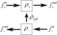
Figure 2: Schematic indicating the flux, probability, and continuity relationships that exist between $\Psi_{\pm}$ components for the CPWM bipolar decompositions considered in this paper. All probability that leaves the $\Psi_{-}$ component must flow into the $\Psi_{+}$ component. Consequently, $\int\left[{\rho_{+}(x)+\rho_{-}(x)}\right]\,dx$ is conserved for all time.

It should be stated that the classical trajectory CPWM bipolar decomposition scheme, in the form described above, is not viable for computing stationary eigenstates below the potential barrier maximum. Tunneling per se is not the issue, since one can in principle apply Eq. (5) in the tunneling regime using analytic continuation (in a manner similar to that applied in paper II) as has been confirmed in numerical tests. However, a difficulty arises when $|p|\rightarrow 0$ and $|p^{\prime}|\rightarrow\infty$, i.e. in the vicinity of the real $x$ axis turning points. For discontinuous potentials, this only occurs for energies near a piece-wise barrier energy $V_{k}$, manifesting as substantially increased propagation times (paper II). For continuous potentials, all energies below the barrier height exhibit turning points along the real $x$ axis, and are therefore problematic. Specifically, the $p^{\prime}$ terms in Eqs. (5) and (6) lead to numerical instabilities near the turning points.

II.3 Exact Quantum Dynamics Using Constant Velocity Trajectories

II.3.1 Motivation

It should be noted that turning point/caustic issues similar to those described in Sec. II.2.3 are also faced by semiclassical methods. Thus, similar remedies may presumably be applied here (e.g. complex plane path deformation), although these are not considered further in this paper. Instead, we are guided by one of our original motivations,poirier04bohmI ; poirier05bohmII to develop methods that avoid such semiclassical difficulties altogether. To this end, we turn once again to the ray optics interpretation of the bipolar approach, as discussed in paper II.

Note that in classical optics, the “ray” interpretation of a given time-evolving electromagnetic field is not necessarily unique; one has a certain freedom to define rays as convenient for a given application.jackson Consider the case of total internal reflection, for instance, at the boundary between two materials with different indices of refraction. Quantum mechanically, this corresponds to a single-step discontinuous potential at an energy below the barrier height (paper II). According to the usual ray interpretation, the incident rays refract to the extent that they become parallel to the interface, and therefore do not penetrate at all into the second medium. This picture is physically somewhat incorrect however, in that it does not capture the exponentially-damped evanescent wave.jackson ; brillouin14 Quantum mechanically, this corresponds to tunneling into the discontinuous step, which is simply not described using the bipolar classical trajectory method as presented in Sec. II.2.

On the other hand, a simple, alternative ray interpretation can be applied to total internal reflection that does predict the evanescent wave correctly. According to this interpretation, the incident ray velocities remain constant across the interface. These rays are reflected within the second medium, giving rise to the evanescent wave, and also providing an explanation for the Goos-Hänchen phenomenon.poirier05bohmII ; jackson ; hirschfelder74 The quantum-mechanical analog would be constant velocity bipolar trajectories, for which the incident wave asymptotic velocities remain constant throughout the interaction region. Presumably, the time evolution equations derived from such a choice of trajectories would not depend very sensitively on the energy $E$, even in the vicinity of the barrier height, so that tunneling, and classical turning points/caustics would pose no special difficulties.

II.3.2 Fröman and Fröman methodology

The semiclassical-like CPWM discussed in Sec. II.2 and the Appendices does not generalize in any straightforward manner for trajectories other than classical. However, there is an alternative time-independent formulation, conceptually similar to the Bremmer (B) approach but differing in the details, which does allow for such a generalization. This approach is due to Fröman and Fröman (F),froman who use it to define generalized semiclassical approximations, although it can also be used to derive corresponding exact quantum bipolar decompositions. The guiding principle of the F approach (as interpreted here) is that semiclassical solutions should satisfy the invariant flux propertypoirier04bohmI ; poirier05bohmII ; froman —i.e., the left side of Eq. (3) with $s^{\prime}_{\text{sc}}(x)$ essentially arbitrary. If $s^{\prime}_{\text{sc}}=p$ is chosen classically, then the usual basic WKB solutions result for $\Psi_{\pm}^{\text{sc}}(x)$. Curiously, however, the corresponding exact quantum $\Psi_{\pm}(x)$ are not the same as in Sec. II.2. In the F case, the decomposition of Eqs. (1) and (4) is uniquely defined via the time-independent Schrödinger equation and the relation

$$\Psi^{\prime} = \alpha_{+}{\left(\Psi_{+}^{\text{sc}}\right)}^{\prime}+\alpha_{-}\left({\Psi_{-}^{\text{sc}}}\right)^{\prime}$$ (8)

$$= -{p^{\prime}\over 2p}\Psi+{ip\over\hbar}\left(\Psi_{+}-\Psi_{-}\right).$$ (9)

Thus, in comparing Eq. (8) to Eq. (4), the $\alpha_{\pm}$ coefficients behave in the derivative as if they were $x$-independent constants, though, in fact, they are not (except when there is no coupling).

Although not identical, the F and B bipolar decompositions are somewhat similar in the classical trajectory case [compare Eq. (9) to Eq. (31)], and both are plagued by similar numerical instabilities near turning points, as has been confirmed in numerical testing. However, the main advantage of the F approach is that it can be applied to arbitrary trajectories, $p$. In particular, we choose constant velocity trajectories obtained from the left-incident plane waves, i.e. $p=\sqrt{2mE}$ [with $\lim_{x\rightarrow-\infty}V(x)=0$]. This gives rise to exact quantum CPWM components $\Psi_{\pm}$ that are smooth and well-behaved everywhere, even near turning points and barrier maxima. Note that for constant velocity trajectories, Eqs. (1) and (9) imply that $\Psi_{\pm}$ are linear combinations of $\Psi$ and $\Psi^{\prime}$.

II.3.3 Time-evolution equations

In analogy with Sec. II.2, the goal is to develop a time-dependent method to compute the F constant velocity CPWM bipolar decomposition in the large $t$ limit. However, since the F construction of the $\Psi_{\pm}$ is radically different from that of B, a substantially different approach than that of Appendix A must be used. We have developed several different derivations, all of which yield the same final results. The simplest strategy is to “work backwards” through Appendix B, but using Eq. (9) for constant velocity trajectories instead of Eq. (31). However, a more pedagogical approach may also be employed, as presented below.

As in Eq. (8), the basic idea is to presume that the coefficients $\alpha_{\pm}$ act as constants, but with respect to time derivatives rather than spatial derivatives. In particular, it seems more natural here to refer to total rather than partial time derivatives, given the trajectory-based nature of the methodology. Less obvious at this stage is the fact that the linear combination $\left(\Psi_{+}-\Psi_{-}\right)$ must be used rather than $\Psi=\Psi_{+}+\Psi_{-}$ itself, in order to be consistent with the time-independent F results. We thus obtain the condition

$${d\Psi_{+}\over dt}-{d\Psi_{-}\over dt} = \alpha_{+}{d\Psi_{+}^{\text{sc}}\over dt}-\alpha_{+}{d\Psi_{+}^{\text{sc}}\over dt}$$ (10)

$$= -{iE\over\hbar}\left(\Psi_{+}-\Psi_{-}\right)+{p\over m}\Psi^{\prime}$$

Together with the time-dependent Schrödinger equation (converted to total derivative form), as applied to the Eq. (1) linear combination, Eq. (10) above gives rise to a unique set of time-evolution equations for $d\Psi_{\pm}/dt$. In the constant velocity trajectory case, for which $\Psi_{\pm}^{\text{sc}}(x,t)\propto\exp\left[{i(\pm\sqrt{2mE}x-Et)/\hbar}\right]$, these are found to be

$${d\Psi_{\pm}\over dt}={i\over\hbar}\left(E-V\right)\Psi_{\pm}-{i\over\hbar}V\Psi_{\mp}.$$ (11)

II.3.4 Additional properties

Using a procedure analogous to that described at the start of Appendix B, one can show that for stationary states, Eq. (11) is in fact consistent with the time-independent F constant velocity CPWM bipolar decomposition. This requires the Eulerian version of Eq. (11), i.e.

$${\partial\Psi_{\pm}\over\partial t}=\mp{p\over m}\Psi_{\pm}^{\prime}+{i\over\hbar}\left(E-V\right)\Psi_{\pm}-{i\over\hbar}V\Psi_{\mp}.$$ (12)

What is not so clear, however, is whether starting with a truncated asymptotic plane wave, one necessarily approaches the stationary solution in the large $t$ limit (Sec. II.2.3, paper II). Although this has not yet been proven, it is a reasonable assumption, given both the counter-propagating trajectory nature of the method and flux properties similar to the B classical trajectory case (discussed below). Moreover, for all of the numerical applications considered in Sec. IV, exponentially fast convergence is in fact observed.

The F constant velocity time-evolution equations [Eq. (11)] offer some decided advantages over the classical trajectory approach. Since only energy quantities appear on the right hand side, there is no need to resort to analytic continuation in order to handle tunneling for the below-barrier energies. The equations may therefore be applied with equal ease throughout the energy spectrum, and in fact, the resultant $\Psi_{\pm}$ are qualitatively similar above, below, and just at the potential barrier maximum (Sec. IV.1). Another advantage is that the numerical propagation does not require spatial differentiation of any kind—not even of the potential, V, to determine forces driving the trajectories. Furthermore, Eq. (11) may be numerically implemented as is for discontinuous potentials, just as easily as for continuous potentials, without the need for explicit splitting and recombining of trajectories as in paper II (Sec. IV.2).

On the other hand, the F constant velocity approach introduces a drawback that the classical trajectory methods do not have to contend with when the potential is “asympotically asymmetric”—by which we mean simply that $\lim_{x\rightarrow-\infty}V(x)=0\neq\lim_{x\rightarrow\infty}V(x)=V_{0}$, corresponding e.g. to an exoergic or endoergic chemical reaction. Whereas in the $x\rightarrow-\infty$ limit, the evolution equations are uncoupled, this is not true in the $x\rightarrow\infty$ limit if $V_{0}\neq 0$, in which case the time-dependent $\Psi_{\pm}$ are not expected to converge. Many techniques could be used to remedy this situation, e.g. trajectories described via smoothly-varying sigmoid (tanh-like) functions rather than uniform or classical trajectories. For purposes of this paper, we adopt a simpler solution, wherein two F constant velocity CPWM bipolar decompositions are used, one each for the reactant and product regions. Standard boundary condition matching techniques are then applied to join these together (Sec. III.3).

Regarding flux properties, Eq. (12) can be used to obtain

$${\partial\rho_{\pm}\over\partial t}=-j_{\pm}^{\prime}\pm{2V\over\hbar}\text{Im}\left[{{\Psi_{+}}^{*}\,\Psi_{-}}\right],$$ (13)

which should be compared with Eq. (7) for the B classical trajectory case. Note that the total combined probability for both $\Psi_{+}$ and $\Psi_{-}$ is conserved here as well, i.e. $\partial(\rho_{+}+\rho_{-})/\partial t=-(j_{+}+j_{-})^{\prime}$, and Fig. 2 still applies. The coupling term $\partial\rho_{\text{cpl}}/\partial t=(2V/\hbar)\text{Im}\left[{{\Psi_{+}}^{*}\,\Psi_{-}}\right]$ is of course different from that of Sec. II.2.3, although in both cases, the wavefunction inner product cross terms are involved. Several additional relations unique to the constant velocity case may also be easily derived from the above equations, e.g.

$$d\rho_{\pm}/dt=\pm\partial\rho_{\text{cpl}}/\partial t,$$ (14)

which states that the probability lost by a positive momentum trajectory is gained by the negative momentum trajectory directly “beneath” it (same $x$), and

$$\rho_{+}^{\prime}=\rho_{-}^{\prime}\quad\text{for stationary solutions},$$ (15)

which states that the positive and negative component density functions are identical apart from a constant. Note that for asymptotically symmetric potentials, and the normalization and boundary conditions described in Secs. II.1 and II.2.2, this constant must be the transmission probability itself, $P_{\text{trans}}$.

III Numerical Details

In this section, we discuss the numerical details associated with implementing the bipolar time-evolution equations of Sec. II as a practical and robust algorithm for computing stationary scattering states. Although any boundary conditions may be considered, our emphasis shall be on left-incident solutions, for which $\Psi_{-}\rightarrow 0$ as $x\rightarrow\infty$. The region of interest is defined via $x_{L}\leq x\leq x_{R}$, a region presumed to include the entire potential interaction to the desired level of accuracy. According to the time-dependent ray optics picture developed in paper II, at the initial time, $\Psi=\Psi_{+}$ is a left-incident plane wave truncated on the right at $x=x_{L}$. This initial wave propagates into the interaction region, wherein it is coupled to $\Psi_{-}$ and eventually reaches a stationary state. Outside of the interaction region, the $\Psi_{\pm}$ coupling may be regarded as effectively zero. Thus, one may compute reflection and transmission probabilities, $P_{\text{refl}}$ and $P_{\text{trans}}$, simply by evaluating $\Psi_{+}(x_{R})$ and $\Psi_{-}(x_{L})$ at sufficiently large times.

From a purely numerical point of view, the above scheme offers many advantages—e.g., the ability to compute specific scattering states without the need for complex scalingcomplexscaling78 ; reinhardt82 ; ryaboy94 or complex absorbing potentialspoirier03capII ; poirier03capI ; jolicard85 ; seideman92a ; riss93 ; muga04 that would increase the coordinate range unnecessarily. Moreover, the density of grid points may be substantially reduced, owing to the fact that the interference-free component functions $\Psi_{\pm}$ are generally smooth and slowly varying as compared to $\Psi$ itself. For the same reason, a larger time-step is also anticipated. Most importantly however, since $q_{\pm}=0$, there is no need to compute on-the-fly numerical spatial derivatives. With regard to parallel computation, therefore, there is no need for trajectories to communicate within a LM, although the coupling requires position-dependent communication between positive and negative LM trajectories.

III.1 Algorithmic Issues

In order to solve the time-evolution equations numerically, two trajectory grids are created, one for each bipolar component of the total wavefunction. Hereafter, “upper” will be used to describe attributes of the $\Psi_{+}$ component, and “lower” for the $\Psi_{-}$ component (e.g. “lower/upper grid,” etc.). On each grid, the corresponding wavefunction component is spatially discretized at the grid point locations and evolved in time.

For the applications considered here, we have found it convenient to modify the ray optics picture somewhat from the form described above and in paper II. First, we define an initial negative LM grid, even though $\Psi_{-}$ itself is zero initially. The idea here is that unlike paper II, we wish to avoid explicit trajectory hopping. Consequently, both sets of grid points exist for all time and evolve independently of each other (though the component wavefunctions do interact). Second, to avoid unnecessary computational effort, no propagation is done outside of the interaction region of interest. Instead, at uniform time intervals, new $\Psi_{+}$ trajectories are fed in at $x=x_{L}$, with an initial $\Psi_{+}$ value consistent with the positive momentum asymptotic plane wave solution. Later, as these upper grid trajectories reach $x=x_{R}$, they are discarded. The $\Psi_{-}$ situation is similar, except that the initial $\Psi_{-}(x_{R})$ value is set to zero, and the trajectories are discarded as they reach $x=x_{L}$.

The most substantial difference from the ray optics picture, however, is found in our implementation of the constant velocity method, for which the grids are distributed uniformly throughout the interaction region at all times. At the initial time, the upper and lower grids coincide. The initial $\Psi_{+}$ is taken to be the asymptotic plane wave solution throughout the interaction region, and the initial $\Psi_{-}$ is set to zero. The above modification, which we call the “non-wavefront” approach, is certainly not necessary, and is introduced simply for convenience. Calculations performed both ways reveal that both converge exponentially to the correct stationary solution. However, the initial convergence of the non-wavefront calculations is faster, owing to the fact that the coupling takes effect immediately. The numerical algorithm is also easier to implement. Consequently, all constant velocity results presented in Sec. IV were obtained using the non-wavefront code.

As per Sec. II, the upper and lower grids move classically or with constant velocity, as appropriate, and the $\Psi_{\pm}$ contributions evolve in accord with Eq. (5) or Eq. (11). Since the grids move in opposite directions, they do not remain commensurate over time. Numerical interpolation (Sec. III.2) is therefore required to compute the coupling contribution from the component wavefunction of one grid to the other. As an alternative to the above trajectory-based (Lagrangian) approach, we have also implemented a fixed-grid (Eulerian) bipolar propagation algorithm for the constant velocity case. The primary advantage of fixed-grid propagation is that the two grids remain commensurate for all time, thus avoiding the need for interpolation. However, this is achieved at the expense of switching to the Eulerian evolution equations [Eq. (12)], which require explicit numerical spatial differentation of the bipolar wavefunction components.

III.2 Low Level Issues

For the numerical propagation of the time-evolution equations, two fourth-order explicit integrators were considered—the multi-step Adam’s/Bashforth, and Runge-Kutta methods.phillips Although, both integrators are fourth-order accurate, and require approximately the same CPU time, multi-step integrators can not be trivially implemented for the asymptotically asymmetric potential case (Sec. III.3). Consequently, the basic fourth-order Runge-Kutta method was used for all results presented herein. In the future, the time integration can be made more accurate by using a time-adaptive Runge-Kutta approach such as the Cash-Carp method.press For most of the calculations performed here, a time-step of $\Delta=10$ a.u. was found to be sufficient to achieve a computed accuracy of $10^{-4}$ or better (Sec. IV). Generally speaking however, the time-step issue is quite problem-dependent, as it can depend on both grid point velocities and spacing.

As discussed in Sec. III.1, the trajectory-based algorithms require interpolation of both bipolar components in order to compute coupling contributions. For all examples considered here, these interpolates were calculated via a polynomial moving least squares (MLS) method.wyatt In MLS methods, local low-order polynomial fits are calculated about each grid point via a small stencil of surrounding neighbor points. To ensure that the fit will exactly represent the function values at the grid point locations, the stencil size and polynomial order must be set equal, thus effectively transforming the MLS method into a moving-interpolation method. For all calculations performed here, five stencil points were used, corresponding to a symmetric stencil (for the interior grid points) and quartic polynomial interpolation.

For the fixed-grid algorithms, explicit numerical spatial differentiation of both CPWM bipolar components must be performed. For the present study, these were calculated using centered, fourth-order finite differencesfornberg88 for the interior grid points, and one-sided fourth-order finite difference for the boundary grid points at $x_{L}$ and $x_{R}$.

III.3 Asymptotically Asymmetric Potentials

As discussed in Sec. II.3.4, the constant velocity time-evolution equations will exhibit coupling in the $x\rightarrow\infty$ asymptote if $V(x)$ is asymptotically asymmetric, i.e. if $\lim_{x\rightarrow\infty}V(x)=V_{0}\neq 0$. To remedy this, we construct two sets of solutions, one for the “reactant” region, $x\leq x_{0}$, and another for the “product” region, $x\geq x_{0}$, with $x_{0}$ the dividing point. For the former solutions (denoted via the “L” subscript), Eq. (11) may be used directly, with $p_{L}=\sqrt{2mE}$. For the product solutions, however (denoted “R”), the evolution equations must be modified slightly to accommodate the generalized asymptotic potential condition,

$${d\Psi_{R\pm}\over dt}={i\over\hbar}\left(E-V-V_{0}\right)\Psi_{R\pm}-{i\over\hbar}\left(V-V_{0}\right)\Psi_{R\mp},$$ (16)

since the positive trajectory momentum is now $p_{R}=\sqrt{2m(E-V_{0})}$. It is clear from Eq. (16) that the coupling vanishes as $x\rightarrow\infty$.

For all propagation times, the wavefunction and its first derivative must be continuous across $x_{0}$. Remarkably, we can treat this boundary condition like an elementary plane wave scattering off a step potential (paper II). This is achieved via Eq. (9), in terms of which the two exact conditions become

$$\Psi_{L+}^{0}+\Psi_{L-}^{0} = \Psi_{R+}^{0}+\Psi_{R-}^{0}$$

$$p_{L}\left[{\Psi_{L+}^{0}-\Psi_{L-}^{0}}\right] = p_{R}\left[{\Psi_{R+}^{0}-\Psi_{R-}^{0}}\right],$$ (17)

where $\Psi_{L+}^{0}=\Psi_{L+}(x_{0})$, etc. In the trajectory-based algorithm, the left and right incident wavefunction values, $\Psi_{L+}^{0}$ and $\Psi_{R-}^{0}$, are known at any given time, whereas the locally transmitted values $\Psi_{R+}^{0}$ and $\Psi_{L-}^{0}$ are unknown. Equation (17) enables one to solve for the two unknowns, and thus to continue propagating trajectories through the dividing point, $x_{0}$.

The solutions are

$$\Psi_{R+}^{0} = \left({2p_{L}\over p_{L}+p_{R}}\right)\Psi_{L+}^{0}+\left({p_{R}-p_{L}\over p_{L}+p_{R}}\right)\Psi_{R-}^{0}$$

$$\Psi_{L-}^{0} = \left({2p_{R}\over p_{L}+p_{R}}\right)\Psi_{R-}^{0}-\left({p_{R}-p_{L}\over p_{L}+p_{R}}\right)\Psi_{L+}^{0},$$ (18)

which do indeed correspond to transmission and reflection coefficients for stationary states of the discontinuous step potential (Appendix A and paper II). Numerically, the propagation is implemented as follows. Equations (11) and (16) are used until a trajectory reaches $x_{0}$, at which point it is replaced with a new trajectory on the other side of $x_{0}$ via Eq. (18). This requires a “known” value from the opposite LM. If the grids are not commensurate (i.e. trajectories from opposite LMs do not arrive at $x_{0}$ at the same time), it is necessary to apply extrapolation to the opposite manifold to determine the “known” value.

IV RESULTS

In this section, four different stationary scattering applications are considered, all with comparable characteristic parameters—e.g., the same proton-like mass of $m=2000$ a.u., barrier height $V_{0}=400\,\text{cm}^{-1}\approx 0.0018$ a.u. (note: $10\times$ smaller than in paper II), and interaction region, $[x_{L}=-3\,\text{a.u.},\,x_{R}=3\,\text{a.u.}]$. All four systems were solved using the non-wavefront, F, constant velocity trajectory-based method, hereinafter referred to as the “constant velocity trajectory” scheme. For the Eckart system (Sec. IV.1), additional calculations were also performed using the constant velocity fixed-grid scheme, and the wavefront, B, classical trajectory method, now referred to as the “classical trajectory” scheme.

IV.1 The Eckart Barrier

The first application considered is the symmetric Eckart problem,eckart30 ; ahmed93 defined via

$$V(x)=V_{0}\,\text{sech}(\alpha x)^{2},$$ (19)

with parameter values $V_{0}=400\,\text{cm}^{-1}$, and $\alpha=3.0$ a.u. The above potential is plotted on the scale of the interaction region in Fig. 3.

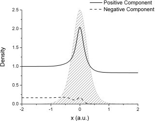
Figure 3: Converged positive component density $\rho_{+}(x)$ (solid line) and negative component density $\rho_{-}(x)$ (dashed line) for the $E=450\,\text{cm}^{-1}$ stationary state of the $V_{0}=400\,\text{cm}^{-1}$ Eckart barrier system, as obtained using the classical trajectory CPWM bipolar decomposition. Shaded area indicates the Eckart potential $V(x)$.

We have performed numerical calculations for the Eckart system using several of the previously described algorithms. In the first study, the classical trajectory scheme was employed, i.e. the continuous potential analog of paper II. A time-step of $\Delta=1$ a.u. was used, and a maximum of 45 trajectories per LM employed at any given time. $P_{\text{refl}}$ and $P_{\text{trans}}$ values were computed for various energies $E>V_{0}$, to a convergence error of $~{}10^{-4}$, and in every case found to match the exact analytical resultsahmed93 to within the same error. A density plot of the CPWM bipolar components for a typical solution ($E=450\,\text{cm}^{-1}\approx 0.002$ a.u.) is presented in Fig. 3. For most energies $E$, these calculations are roughly as efficient as the constant velocity calculations described below. However, the required propagation time does indeed increase rapidly as $E\rightarrow V_{0}$, as expected. In this limit, the classical trajectory bipolar decomposition also becomes unstable; the small central peaks evident in Fig. 3 become increasingly pronounced, eventually developing into singularities.

The second study is a detailed convergence and efficiency comparison between the trajectory and fixed-grid implementations of the constant velocity method (Sec. III.1). This study also serves as a benchmark for establishing the numerical parameter values needed to achieve a $10^{-4}$ accuracy level. Both schemes were applied to a calculation of the $E=V_{0}$ stationary state, i.e. the classical “worst-case scenario,” for a varying number of grid points, $N$. A time-step of $\Delta=1$ a.u. was used for the trajectory calculation, and $\Delta=0.1$ a.u. in the fixed-grid case. Both calculations were propagated to time $t_{\text{max}}=10,000$ a.u. These parameters were sufficiently converged as to ensure that their contribution to the total numerical error is insignificant (i.e. $~{}10^{-8}$ or less). In Fig. 4, the resultant CPU times on a 2.60 GHz Pentium computer are presented. Note that despite the ten-fold increase in the number of time-steps for the fixed-grid case, the total CPU time is still markedly faster for all grid sizes considered. This is due both to the search operation (to find the nearest opposite LM trajectories) and the interpolation matrix inversions required at each time-step by the trajectory scheme.

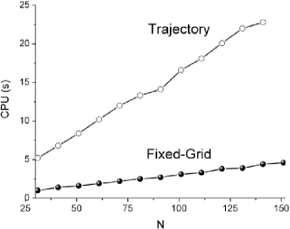
Figure 4: CPU time vs. no. of grid points, $N$, required to propagate trajectory (empty circles) and fixed-grid (filled circles) implementations of the constant velocity CPWM bipolar decomposition to a final system time of $t_{\text{max}}=10,000$ a.u. The trajectory and fixed grid time-steps used were $\Delta=1$ a.u. and $\Delta=0.1$ a.u., respectively.

In Fig. 5, the log of the computed $P_{\text{refl}}$ and $P_{\text{trans}}$ errors (relative to known analytical valuesahmed93 ) are plotted versus $N$. Across $N$, the trajectory-based results are seen to be much more accurate than the fixed-grid results, although the latter are substantially improved by increasing the density of grid points. For example, in order to achieve $10^{-4}$ accuracy for both $P_{\text{refl}}$ and $P_{\text{trans}}$, only $N=25$ trajectories were needed, whereas $N=91$ fixed-grid points were required. This is consistent with the fixed-grid method requiring explicit spatial differentiation, introducing an additional source of numerical error. Note that for this comparison, the CPU times are comparable—4.3 seconds and 2.7 seconds, respectively. The fixed-grid calculation is slightly faster, although this situation would be reversed for more accurate calculations (e.g. $10^{-6}$) and/or higher dimensionalities. The performance of both methods is in any event remarkable, with the large-$N$ trajectory case representative of the most accurate trajectory-based quantum scattering calculations performed to date. Further improvements are also possible, however, as discussed in Sec. III.2.

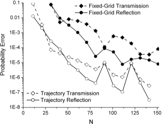
Figure 5: Errors in computed reflection probabilities $P_{\text{refl}}$ (solid lines) and transmission probabilities $P_{\text{trans}}$ (dashed lines) vs. no. of grid points $N$ for the $E=400\,\text{cm}^{-1}$ stationary state of the $V_{0}=400\,\text{cm}^{-1}$ Eckart barrier system, as obtained using trajectory and fixed-grid implementations of the constant velocity CPWM bipolar decomposition. Errors are relative to known analytical results (Ref. [47]).

The final study was a constant velocity trajectory calculation of $P_{\text{refl}}$ and $P_{\text{trans}}$ over a wide range of $E$ values—including those above, below, and at the barrier maximum, $E=V_{0}$. The parameters $\Delta=10$ a.u., $t_{\text{max}}=10,000$ a.u., and $N=31$ were chosen to correspond to a target accuracy of $~{}10^{-4}$. The resulting stationary state solution for the $E=V_{0}$ case is displayed in Figs. 6 and 7. Note the contrast between the smooth, slowly-varying CPWM bipolar densities $\rho_{\pm}$ in Fig. 6 vs. the oscillatory total density $\rho$ of Fig. 7. Nevertheless, as indicated in the latter figure, the numerically reconstructed total density agrees with the analytical resultahmed93 to within the target accuracy of $10^{-4}$ at all grid points. Note also that $\rho_{+}$ and $\rho_{-}$ are identical apart from a constant, as predicted in Sec. II.3.4.

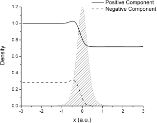
Figure 6: Converged positive component density $\rho_{+}(x)$ (solid line) and negative component density $\rho_{-}(x)$ (dashed line) for the $E=400\,\text{cm}^{-1}$ stationary state of the $V_{0}=400\,\text{cm}^{-1}$ Eckart barrier system, as obtained using the constant velocity trajectory CPWM bipolar decomposition. Shaded area indicates the Eckart potential $V(x)$.

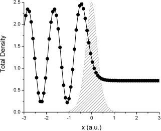
Figure 7: Total wavefunction density $\rho(x)$ for the $E=400\,\text{cm}^{-1}$ stationary state of the $V_{0}=400\,\text{cm}^{-1}$ Eckart barrier system, as obtained using the constant velocity trajectory CPWM bipolar decomposition (filled circles), and compared with exact analytical results (solid line). Shaded area indicates the Eckart potential $V(x)$.

For all 26 energy values considered, the resulting constant velocity bipolar decompositions are qualitatively similar to those presented here for $E=V_{0}$. Indeed, in no respect do these calculations seem to depend sensitively on the value of $E$, unlike the classical trajectory case. Consequently, the same numerical parameters as described above were used for all energies. The resulting computed $P_{\text{refl}}$ and $P_{\text{trans}}$ values are presented in Fig. 8 and compared with analytical values. Once again, all errors are found to be smaller than $10^{-4}$.

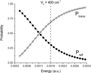
Figure 8: Computed reflection probabilities $P_{\text{refl}}$ (filled circles) and transmission probabilities $P_{\text{trans}}$ (empty circles) vs energy $E$ for the $V_{0}=400\,\text{cm}^{-1}$ Eckart barrier system, as obtained using the constant velocity trajectory CPWM bipolar decomposition, and compared with exact analytical results (solid line).

IV.2 The Square Barrier

Although the primary focus of this paper is continuous potentials, it is worth emphasizing that the methods presented here may be applied to discontinuous potentials as well. As a case in point, we reexamine the square barrier system introduced in paper II. Note that the classical trajectory scheme for $E>V_{0}$ would yield results identical to those of paper II, as is easily verified from Eq. (5). Instead, we focus on the constant velocity trajectory scheme, which can be applied directly without any algorithmic modification.

For the following square barrier study, we used a barrier height of $V_{0}=400\,\text{cm}^{-1}$, and barrier edges of $x_{1}=-1$ and $x_{2}=1$, respectively. As in Sec. IV.1, $N=31$ initial grid points were distributed uniformly throughout the interaction region, and the time-step was defined as $\Delta=10$ a.u. The energy was taken to be $E=450\,\text{cm}^{-1}\approx 0.002$ a.u., i.e. slightly above-barrier. The propagation was continued until the computed $P_{\text{refl}}$ and $P_{\text{trans}}$ values were both converged to less than $10^{-4}$, which was found to require approximately 1000 time-steps.

Figure 9 is a density plot of the converged CPWM bipolar component solutions. As in the Eckart case, the results are well-behaved and interference-free throughout, although there is a discontinuity in the first spatial derivative at the step edges (but not for the total $\Psi$ itself). For the total density $\rho$, the computed values and the analytical results are once again in agreement to $10^{-4}$ or better, at all grid points.

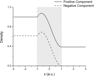
Figure 9: Converged positive component density $\rho_{+}(x)$ (solid line) and negative component density $\rho_{-}(x)$ (dashed line) for the $E=450\,\text{cm}^{-1}$ stationary state of the $V_{0}=400\,\text{cm}^{-1}$ square barrier system, as obtained using the constant velocity trajectory CPWM bipolar decomposition. Shaded area indicates the square barrier potential $V(x)$

The calculation described above was repeated for a total of 45 different energy values. The resultant converged $P_{\text{refl}}$ and $P_{\text{trans}}$ values are presented in Fig. 10, as are the exact analytical results. Relative to the latter, all computed probability errors are found to be less than $10^{-4}$.

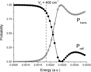
Figure 10: Computed reflection probabilities $P_{\text{refl}}$ (filled circles) and transmission probabilities $P_{\text{trans}}$ (empty circles) vs energy $E$ for the $V_{0}=400\,\text{cm}^{-1}$ square barrier system, as obtained using the constant velocity trajectory CPWM bipolar decomposition, and compared with exact analytical results (solid line).

IV.3 The Uphill Ramp

The next application considered is an asymptotically asymmetric system—the continuous “uphill ramp”flugge defined via

$$V(x)={V_{0}\over 2}\left[{1+\tanh\left({x\over 2\alpha}\right)}\right],$$ (20)

with the parameters $V_{0}=400\,\text{cm}^{-1}$ and $\alpha=0.2$ a.u. This is another scattering system that is analytically soluble.flugge Note that $\lim_{x\rightarrow-\infty}V(x)=0$ and $\lim_{x\rightarrow\infty}V(x)=V_{0}$, as presumed in Sec. III.3.

The propagation was performed using the constant velocity trajectory scheme described in Sec. III.3, with the dividing point chosen to be $x_{0}=0$. All other computational parameters were identical to those of the previous examples, except for the energy, which was chosen to be $E=500\,\text{cm}^{-1}\approx 0.0023$ a.u. Again, the propagation was continued until both $P_{\text{refl}}$ and $P_{\text{trans}}$ were converged to less than $10^{-4}$. Figure 11 is a density plot of the resultant CPWM bipolar component solutions. There is a discontinuity at $x_{0}=0$, which is to be expected given the “step-like” nature of the join (the same behavior is observed in paper II). Importantly, however, this discontinuity does not give rise to any numerical problems, since spatial derivatives are not required in the trajectory integration (though one must be a bit careful with the interpolation). Away from $x_{0}$, both density plots are smooth and well-behaved.

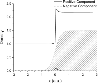
Figure 11: Converged positive component density $\rho_{+}(x)$ (solid line) and negative component density $\rho_{-}(x)$ (dashed line) for the $E=500\,\text{cm}^{-1}$ stationary state of the $V_{0}=400\,\text{cm}^{-1}$ uphill ramp system, as obtained using the constant velocity trajectory CPWM bipolar decomposition, modified for asymptotically asymmetric potentials. The dividing point is $x_{0}=0$. Shaded area indicates the uphill ramp potential $V(x)$.

Despite the discontinuities in $\rho_{\pm}$, the computed $\rho$ and its first derivative are continuous, owing to the Eq. (18) relations. This is evident in Fig. 12, a density plot for the converged total $\Psi$. As is clear from the plot, no visible discrepancies may be observed between the computed and analytically exact solutions.

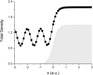
Figure 12: Total wavefunction density $\rho(x)$ for the $E=500\,\text{cm}^{-1}$ stationary state of the $V_{0}=400\,\text{cm}^{-1}$ uphill ramp system, as obtained using the constant velocity trajectory CPWM bipolar decomposition (filled circles), and compared with exact analytical results (solid line, Ref. [48]). Shaded area indicates the uphill ramp potential $V(x)$.

IV.4 The Double-Gaussian Barrier

The previous three example systems serve as useful benchmarks for testing and evaluating the new bipolar methodologies under a wide range of conditions. In particular, all three have known analytical solutions, against which the computed results may be compared. However, we feel it is also worthwhile to consider at least one system which has not previously been solved. One such example, which also presents a qualitatively new variety of problem, is the symmetric double-Gaussian barrier potential,

$$V(x)=V_{0}\left\{\exp\left[{-\beta\left(x-x_{0}\right)^{2}}\right]+\exp\left[{-\beta\left(x+x_{0}\right)^{2}}\right]\right\}.$$ (21)

For the results presented here, the following parameters were used: $V_{0}=400\,\text{cm}^{-1}$; $\beta=9$ a.u.; $x_{0}=0.75$ a.u.

Once again, the constant velocity trajectory method was employed, with the same computational parameters as described previously. The energy was chosen to be just at the barrier height, $E=V_{0}$. Figure 13 displays the resulting converged CPWM bipolar densities. As in the previous examples, these are identical apart from a constant, and are otherwise smooth and slowly-varying. Note that the double-barrier nature of the potential gives rise to interesting features in the bipolar densities not previously observed. In particular, despite the fact that $V(x)$ is changing in the central well region between the two barriers, the bipolar densities are nearly flat across this region, resulting in a well-defined “reaction intermediate” state between reactants and products. Moreover, the density plots enable one to assign quantitative probability values for the intermediate state.

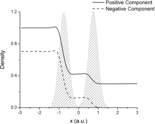
Figure 13: Converged positive component density $\rho_{+}(x)$ (solid line) and negative component density $\rho_{-}(x)$ (dashed line) for the $E=400\,\text{cm}^{-1}$ stationary state of the $V_{0}=400\,\text{cm}^{-1}$ double-Gaussian barrier system, as obtained using the constant velocity trajectory CPWM bipolar decomposition. Shaded area indicates the double-Gaussian potential, $V(x)$.

In contrast, the above interpretation and quantitative assignments would be very difficult, if not impossible, to glean directly from $\Psi(x)$ itself. This is evident from Fig. 14, a density plot of the total $\Psi$ for the above double-Gaussian barrier calculation, obtained via interpolation and superposition of the two converged bipolar component solutions, $\Psi_{\pm}$. Note the interference present both in the reactant region (due to reflected trajectories) and the intermediate region. Thus, not only the intermediate probabilities, but also the reflection probability, are difficult to read directly from such a plot.

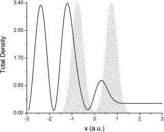
Figure 14: Total wavefunction density $\rho(x)$ (solid line) for the $E=400\,\text{cm}^{-1}$ stationary state of the $V_{0}=400\,\text{cm}^{-1}$ double-Gaussian barrier system, as obtained using the constant velocity trajectory CPWM bipolar decomposition. Shaded area indicates the double-Gaussian potential, $V(x)$.

V SUMMARY AND CONCLUSIONS

Scattering applications are of paramount importance for chemical reactions, because all reactions may be regarded as scattering events. From a theoretical exact quantum perspective, therefore, multichannel scattering theory,taylor both time-dependent and time-independent, will always play an essential role. At the same time however, trajectory-based methods also bring much to bear on dynamics, providing great insight into reactive processes, vis-a-vis the determination of which trajectories make it past the barrier to products vs. those that do not. Quantum trajectory methods (QTMs) therefore exhibit great potential promise as a chemical dynamics tool, combining a trajectory-based description with exact quantum dynamics. However, all reactive systems exhibit interference between the incident and reflected (non-reactive) waves, thus causing numerical instability problems for conventional unipolar QTMs. CPWM bipolar decompositions offer a natural means of alleviating this interference difficulty, by splitting the reactant region $\Psi$ into incident $\Psi_{+}$ and reflected $\Psi_{-}$ components, neither of which exhibits interference on its own. Moreover, this splitting can be extended through the interaction region over to the product region, by which point $\Psi_{+}$ has transformed smoothly into the transmitted wave, and $\Psi_{-}$ has damped to zero.

As discussed in Sec. II and the Appendices, the CPWM approach borrows conceptually from semiclassical scattering methods. Indeed, for the first bipolar decomposition considered (B, Sec. II.2) the bipolar trajectories are simply equal to the classical trajectories themselves, and the correspondence principle is satisfied in precisely the usual WKB limit, $V^{\prime}\rightarrow 0$. Three features, however, contribute to render the present approach fundamentally different from basic WKB theory: (1) time-dependent formulation; (2) coupling between $\Psi_{+}$ and $\Psi_{-}$; (3) universal, local reflection and transmission formulae (see also paper II). Point (3) is what determines point (2), i.e. if only local transmission were considered without reflection, then the coupling would vanish and the basic WKB solutions would result. The combination of (1) and (3) provides a local physical understanding related to the ray optics picture in electromagnetic theory, and also gives rise to useful flux relations and numerical algorithms. Regarding the second bipolar decomposition considered, i.e. the F, constant velocity scheme, this was motivated by practical concerns, but also by an alternative ray optics description (Sec. II.3). This can be related to the semiclassical approach of Fröman and Fröman, and in that context, also satisfies a generalized kind of correspondence principle.

Note that neither set of evolution equations [Eqs. (5) and (11)] involves a quantum potential; instead, all quantum effects manifest through $\Psi_{\pm}$ coupling. In both cases, the trajectories themselves are not “context-sensitive,”wyatt in that they may be computed independently of the $\Psi_{\pm}$ evolution. Moreover, no spatial differentiation of the wavefunction is required, although there may be situations where explicit calculation of one spatial derivative is numerically advantageous (Sec. IV.1). Several other numerical modifications have also been introduced for convenience (Sec. III.1), resulting in a shift from an exact time-dependent Schrödinger interpretation of the dynamics [wherein the exact stationary state is “revealed” over time (paper II)] to what may be regarded as more of a relaxation approach. Be that as it may, the resulting algorithms offer a remarkably simple, efficient, and accurate means of performing reactive scattering calculations of all kinds in 1D (Sec. IV). Indeed, the time-steps required for the benchmark molecule-like systems considered here are orders of magnitude larger than for typical fixed-grid calculations performed at a comparable level of accuracy. Moreover, the converged bipolar solution density plots render the determination of global reflection and transmission probabilities, as well as probabilities for reaction intermediate states, quite straightforward.

In future publications we will continue to generalize the methodology described here and in paper II, for the type of multidimensional time-dependent wavepacket dynamics relevant to real chemical physics applications. As additional motivation for the present work, we now sketch how this might be achieved. First, it is necessary to generalize the stationary state results of this paper and paper II for arbitrary time-evolving wavepackets. This is done initially for the discontinuous step potential, and then generalized for arbitrary continuous potentials in a manner similar to Appendix A. In fact, much of the groundwork is already laid, in that the time-dependent framework has already been introduced.

The generalization to multidimensional systems is less straightforward but can certainly be achieved (such calculations have already been performed, as will be reported in a future publication). Conceptually at least, many direct chemical reactions can be described using a single scattering reaction coordinate, plus additional “bound” coordinates. It is natural to consider applying the current CPWM bifurcation to the former, and the paper I bifurcation to each of the latter. However, the total number of wavefunction components would then be $2^{D}$ where $D$ is the number of degrees of freedom. On the other hand, for most time-dependent wavepacket calculations, node formation in $\Psi$ is associated primarily with the reaction coordinate itself, due to wavepacket reflection off of the reaction profile barrier. Thus, a natural approach would be to bifurcate only along the reaction coordinate. Only two component wavefunctions result, regardless of $D$. It remains to be seen whether such a procedure will render QTM calculations possible for actual molecular systems. Nevertheless, it seems very likely that some such bipolar or multipolar approach will go a long way towards ameliorating the infamous node problem, which has thus far severely limited the effectiveness of QTMs in the molecular arena.

Appendix A Derivation of bipolar time-evolution equations

Following the notation of paper II, Sec. II D 3, we presume a discontinuous potential, for which $x_{k}$ ($k=1,2,\ldots,l$) denote the locations of the $l$ discontinuities. The $x_{k}$ divide configuration space into $l+1$ regions, labeled $0\leq k\leq l$. In each region $k$, the potential has a different constant value, $V_{k}$. The discontinuous system described above may be used to model any continuous potential system, $V(x)$, by defining $V_{k}=V(x_{k}^{m})$ [where $x_{k}^{m}=(x_{k}+x_{k+1})/2$ is the region midpoint] and taking the limit that $(x_{k+1}-x_{k})\rightarrow 0$ for all $k$.

As the derivation is a time-dependent one, it is convenient to introduce a small (ultimately differential) time increment $\Delta$, which is then used to determine the $x_{k}$ as follows. Associated with each region $k$ is the positive classical momentum value, $p_{k}=\sqrt{2m\left[{E-V_{k}}\right]}$ [i.e. $p_{+}^{\text{sc}}(x_{k}^{m})$]. The $x_{k}$ are chosen such that a particle moving with momentum $p_{k}$ would traverse the region $k$ in time $\Delta$, i.e. $(x_{k+1}-x_{k})=\Delta(p_{k}/m)$. Consider a trajectory which at $t=0$, is located at the $k$’th region midpoint, $x_{k}^{m}$, heading to the right with momentum $p_{k}$. This is clearly a positive LM trajectory, carrying a contribution of the component wavefunction $\Psi_{+k}=\Psi_{+}(x=x_{k}^{m},t=0)$ (Fig. 1). It is presumed that there are also negative LM trajectories along which $\Psi_{-}$ is propagated, but for now the emphasis is on $\Psi_{+}$.

From $t=0$ to $t=\Delta/2$, the positive LM trajectory travels from $x=x_{k}^{m}$ to the discontinuity at $x=x_{k+1}$. As per paper II, the propagation is that of a plane wave, i.e.

$$\Psi_{+k} \rightarrow \Psi_{+}(x_{k+1},\Delta/2)$$ (22)

$$=\Psi_{+k}\exp\left({i\Delta\over 2\hbar}\left[{{p_{k}^{2}\over 2m}-V_{k}}\right]\right)$$

$$=\Psi_{+k}\exp\left({i\Delta\over 2\hbar}\left[{E-2V_{k}}\right]\right).$$

At this point, the trajectory splits into two: one that continues in the forward direction along the positive LM, transmitting into region $k+1$ with momentum $p_{k+1}$; the other reflected backwards along the negative LM with momentum $-p_{k}$ (Fig. 1). According to paper II Eqs. (17) and (18), the trajectory bifurcation introduces a factor of $2p_{k}/(p_{k}+p_{k+1})$ into the the transmitted $\Psi_{+}$ wave, and $(p_{k}-p_{k+1})/(p_{k}+p_{k+1})$ into the reflected $\Psi_{-}$ wave.

During the remaining time evolution from $t=\Delta/2$ to $t=\Delta$, the $\Psi_{+}$ trajectory moves to $x_{k+1}^{m}$ [the midpoint of the adjacent $(k+1)$’th region], resulting in an additional phase factor analogous to that of Eq. (22). The final result is

$$\Psi_{+k}\rightarrow\Psi_{+}(x_{k+1}^{m},\Delta)$$ (23)

$$=\Psi_{+k}\exp\left({i\Delta\over\hbar}\left[{E-V_{k}-V_{k+1}}\right]\right)\left({2p_{k}\over p_{k}+p_{k+1}}\right).$$

The reflected trajectory, meanwhile, moves back to the original location at $x_{k}^{m}$, resulting in the following for $\Psi_{-}$:

$$\Psi_{+k}\rightarrow\Psi_{-}(x_{k}^{m},\Delta)$$ (24)

$$=\Psi_{+k}\exp\left({i\Delta\over\hbar}\left[{E-2V_{k}}\right]\right)\left({p_{k}-p_{k+1}\over p_{k}+p_{k+1}}\right).$$

We thus find that $\Psi_{+k}$ at time $t=0$ contributes to both $\Psi_{+(k+1)}$ and $\Psi_{-k}$ at time $t=\Delta$. However, these must be combined with similar contributions from the initial $\Psi_{-(k+1)}$ in order to determine the total final $\Psi_{+(k+1)}$ and $\Psi_{-k}$ (Fig. 1). Following an analysis similar to the above, the negative LM contributions are easily shown to be the following:

$$\Psi_{-(k+1)}\rightarrow\Psi_{+}(x_{k+1}^{m},\Delta)$$ (25)

$$=-\Psi_{-(k+1)}\exp\left({i\Delta\over\hbar}\left[{E-2V_{k+1}}\right]\right)\left({p_{k}-p_{k+1}\over p_{k}+p_{k+1}}\right).$$

$$\Psi_{-(k+1)}\rightarrow\Psi_{-}(x_{k}^{m},\Delta)$$ (26)

$$=\Psi_{-(k+1)}\exp\left({i\Delta\over\hbar}\left[{E-V_{k}-V_{k+1}}\right]\right)\left({2p_{k+1}\over p_{k}+p_{k+1}}\right).$$

By adding Eqs. (A) and (25), we obtain the final expression for $\Psi_{+}(x_{k+1}^{m},\Delta)$. Subtracting $\Psi_{+k}$, dividing by $\Delta$, and taking the limit $\Delta\rightarrow 0$ yields the total (hydrodynamic) time derivative, $d\Psi_{+}/dt$. We thus obtain

$$\lim_{\Delta\rightarrow 0}\left[{{\Psi_{+}(x_{k+1}^{m},\Delta)-\Psi_{+k}\over\Delta}}\right]=$$

$$\lim_{\Delta\rightarrow 0}\Bigg{\{}\Bigg{.}\bigg{[}{1\over\Delta}\left({p_{k}-p_{k+1}\over p_{k}+p_{k+1}}\right)+{i\over\hbar}\left(E-V_{k}-V_{k+1}\right)$$

$$\times\left({2p_{k}\over p_{k}+p_{k+1}}\right)\Bigg{.}\Bigg{]}\Psi_{+k}-\left[{{1\over\Delta}+{i\over\hbar}\left(E-2V_{k+1}\right)}\right]$$

$$\times\left({p_{k}-p_{k+1}\over p_{k}+p_{k+1}}\right)\Psi_{-(k+1)}\Bigg{.}\Bigg{\}}.$$ (27)

Recall that $\Delta=(x_{k+1}-x_{k})m/p_{k}$. In the small $\Delta$ limit, $V_{k+1}\rightarrow V_{k}$, $p_{k+1}\rightarrow p_{k}$, and $-(p_{k}-p_{k+1})/(x_{k+1}-x_{k})\rightarrow p^{\prime}(x)=\partial p(x)/\partial x$. Substituting into Eq. (A), and replacing $k$ subscripts with functions of $x=x_{k}$ yields:

$${d\Psi_{+}\over dt}=\left[{-{p^{\prime}\over 2m}+{i\over\hbar}\left(E-2V\right)}\right]\Psi_{+}+{p^{\prime}\over 2m}\Psi_{-}$$ (28)

A similar analysis applied to Eqs. (A) and (26) yields:

$${d\Psi_{-}\over dt}=\left[{{p^{\prime}\over 2m}+{i\over\hbar}\left(E-2V\right)}\right]\Psi_{-}-{p^{\prime}\over 2m}\Psi_{+}$$ (29)

Appendix B Proof that bipolar stationary solutions satisfy time-independent Schrödinger equation

Consider the stationary solutions of Eq. (6), i.e. $\partial\Psi_{\pm}/\partial t=-(i/\hbar)E\Psi_{\pm}$. Substituting in these expressions for the time derivatives, and rewriting to obtain expressions for the spatial derivatives, yields:

$$\Psi_{\pm}^{\prime}=\left(-{p^{\prime}\over 2p}\pm{ip\over\hbar}\right)\Psi_{\pm}+{p^{\prime}\over 2p}\Psi_{\mp}$$ (30)

These equations are identical to those of the bipolar time-independent stationary state decomposition described in LABEL:berry72. Adding the ${\Psi_{+}}^{\prime}$ and ${\Psi_{-}}^{\prime}$ equations together results in

$$\Psi^{\prime}={ip\over\hbar}\left(\Psi_{+}-\Psi_{-}\right).$$ (31)

Applying spatial differentiation and substituting Eq. (30) into the resulting right hand side yields $\Psi^{\prime\prime}=-(p^{2}/\hbar^{2})\Psi$. Substitution into the Schrödinger equation then results in

$$-{\hbar^{2}\over 2m}\Psi^{\prime\prime}+V\Psi={p^{2}\over 2m}\Psi+V\Psi=E\Psi.$$ (32)

The stationary solutions of Eq. (6) are therefore consistent with the time-independent Schrödinger equation.

References

- (1) B. Poirier, J. Chem. Phys. 121, 4501 (2004).
- (2) B. Poirier, J. Chem. Phys. , (in press).
- (3) D. Babyuk and R. E. Wyatt, J. Chem. Phys. 121, 9230 (2004).
- (4) R. E. Wyatt, Quantum Dynamics with Trajectories: Introduction to Quantum Hydrodynamics (Springer, New York, 2005).
- (5) C. L. Lopreore and R. E. Wyatt, Phys. Rev. Lett. 82, 5190 (1999).
- (6) F. S. Mayor, A. Askar, and H. A. Rabitz, J. Chem. Phys. 111, 2423 (1999).
- (7) R. E. Wyatt, Chem. Phys. Lett. 313, 189 (1999).
- (8) D. V. Shalashilin and M. S. Child, J. Chem. Phys. 113, 10028 (2000).
- (9) R. E. Wyatt and E. R. Bittner, J. Chem. Phys. 113, 8898 (2001).
- (10) R. E. Wyatt and K. Na, Phys. Rev. E 65, 016702 (2001).
- (11) I. Burghardt and L. S. Cederbaum, J. Chem. Phys. 115, 10312 (2001).
- (12) E. R. Bittner, J. B. Maddox, and I. Burghardt, Int. J. Quantum Chem. 89, 313 (2002).
- (13) K. H. Hughes and R. E. Wyatt, Phys. Chem. Chem. Phys. 5, 3905 (2003).
- (14) E. Madelung, Z. Phys. 40, 322 (1926).
- (15) J. H. van Vleck, Proc. Natl. Acad. Sci. U.S.A. 14, 178 (1928).
- (16) D. Bohm, Phys. Rev. 85, 166 (1952).
- (17) D. Bohm, Phys. Rev. 85, 180 (1952).
- (18) T. Takabayasi, Prog. Theor. Phys. 11, 341 (1954).
- (19) P. R. Holland, The Quantum Theory of Motion (Cambridge University Press, Cambridge, 1993).
- (20) E. R. Floyd, Physics Essays 7, 135 (1994).
- (21) M. R. Brown, arXiv:quant-ph/0102102 (2002).
- (22) J. R. Taylor, Scattering Theory (John Wiley & Sons, Inc., New York, NY, 1972).
- (23) J. Heading, An Introduction to Phase-integral Methods (Methuen, London, 1962).
- (24) N. Fröman and P. O. Fröman, JWKB Approximation (North-Holland, Amsterdam, 1965).
- (25) M. V. Berry and K. V. Mount, Rep. Prog. Phys. 35, 315 (1972).
- (26) J. B. Keller and S. I. Rubinow, Ann. Phys. 9, 24 (1960).
- (27) V. P. Maslov, Théorie des Perturbations et Méthodes Asymptotiques (Dunod, Paris, 1972).
- (28) R. G. Littlejohn, J. Stat. Phys. 68, 7 (1992).
- (29) M. S. Child, Molecular Collision Theory (Dover, New York, 1996).
- (30) B. Poirier and T. Carrington, Jr., J. Chem. Phys. 119, 77 (2003).
- (31) H. Bremmer, Commun. Pure Appl. Math. 4, 105 (1951).
- (32) B. Poirier and T. Carrington, Jr., J. Chem. Phys. 118, 17 (2003).
- (33) J. D. Jackson, Classical Electrodynamics, 2nd ed. (John Wiley & Sons, New York, 1975).
- (34) L. Brillouin, Ann. Phys. 44, 177 (1914).
- (35) J. O. Hirschfelder, A. C. Christoph, and W. E. Palke, J. Chem. Phys. 61, 5435 (1974).
- (36) see for example, Int. J. Quant. Chem. 14, (1978), special issue.
- (37) W. P. Reinhardt, Ann. Rev. Phys. Chem. 33, 223 (1982).
- (38) V. Ryaboy, N. Moiseyev, V. A. Mandelshtam, and H. S. Taylor, J. Chem. Phys. 101, 5677 (1994).
- (39) G. Jolicard and E. J. Austin, Chem. Phys. Lett. 121, 106 (1985).
- (40) T. Seideman and W. H. Miller, J. Chem. Phys. 96, 4412 (1992).
- (41) U. V. Riss and H.-D. Meyer, J. Phys. B: At. Mol. Phys. 26, 4503 (1993).
- (42) J. G. Muga, J. P. Palao, B. Navarro, and I. L. Egusquiza, Phys. Rep. 395, 357 (2004).
- (43) G. M. Phillips and P. J. Taylor, Theory and Applications of Numerical Analysis (Academic Press, New York, 1996).
- (44) W. H. Press et al, in Numerical Recipes, 1st ed. (Cambridge University Press, Cambridge, England, 1989).
- (45) B. Fornberg, Math. Comp. 51, 699 (1988).
- (46) C. Eckart, Phys. Rev. 35, 1303 (1930).
- (47) Z. Ahmed, Phys. Rev. A 47, 4761 (1993).
- (48) S. Flugge, Practical Quantum Mechanics (Springer-Verlag, New York, 1971), Vol. 1.