Smectic-$C$ tilt under shear in smectic-$A$ elastomers

Abstract

Stenull and Lubensky [Phys. Rev. E 76, 011706 (2007)] have argued that shear strain and tilt of the director relative to the layer normal are coupled in smectic elastomers and that the imposition of one necessarily leads to the development of the other. This means, in particular, that a Smectic-$A$ elastomer subjected to a simple shear will develop Smectic-$C$-like tilt of the director. Recently, Kramer and Finkelmann [arXiv:0708.2024, Phys. Rev. E 78, 021704 (2008)] performed shear experiments on Smectic-$A$ elastomers using two different shear geometries. One of the experiments, which implements simple shear, produces clear evidence for the development of Smectic-$C$-like tilt. Here, we generalize a model for smectic elastomers introduced by Adams and Warner [Phys. Rev. E 71, 021708 (2005)] and use it to study the magnitude of Sm$C$-like tilt under shear for the two geometries investigated by Kramer and Finkelmann. Using reasonable estimates of model parameters, we estimate the tilt angle for both geometries, and we compare our estimates to the experimental results. The other shear geometry is problematic since it introduces additional in-plane compressions in a sheet-like sample, thus inducing instabilities that we discuss.

I Introduction

Smectic elastomers WarnerTer2003 are rubbery materials with the orientational properties of smectic liquid crystals deGennesProst93_Chandrasekhar92 . They possess a plane-like, lamellar modulation of density in one direction. In the smectic-$A$ (Sm$A$) phase, the Frank director $\bm{{\rm n}}$ describing the average orientation of constituent mesogens is parallel to the normal $\bm{{\rm k}}$ of the smectic layers whereas in the smectic-$C$ (Sm$C$) phase, there is a non-zero tilt-angle $\Theta$ between $\bm{{\rm n}}$ and $\bm{{\rm k}}$.

Recently, there has been some controversy about whether shear strain and tilt of the director relative to the layer normal are coupled in smectic elastomers and whether the imposition of one necessarily leads to the development of the other. Beautiful experiments by Nishikawa and Finkelmann nishikawa_finkelmann_99 , where a Sm$A$ elastomer was subjected to extensional strain along the layer normal, found a drastic decrease in Young’s modulus at a threshold strain of about $3\%$ accompanied by a rotation of $\bm{{\rm k}}$ through an angle $\varphi$ that sets in at the same threshold. Interpreting their x-ray data, the authors concluded that there was no Sm$C$-like order over the range of strains they probed, and that the reduction in Young’s modulus stems from a partial breakdown of smectic layering. Recently, Adams and Warner (AW) adams_warner_2005 developed a model for Sm$A$ elastomers which assumes that $\bm{{\rm n}}$ and $\bm{{\rm k}}$ are rigidly locked such that $\Theta=0$. This model produces a stress-strain curve and a curve for the rotation angle $\varphi$ of $\bm{{\rm k}}$ in full agreement with the experimental curves but without needing to invoke a breakdown of smectic layering. Evidently, because of the assumption $\Theta=0$, the AW model predicts no Sm$C$-like order. More recently, Stenull and Lubensky StenLubSmA2007 argued that shear strain and Sm$C$-like order are coupled and that the imposition of one inevitably leads to the development of the other. They developed a model based on Lagrangian elasticity that predicts, as does the AW model, a stress-strain curve and a curve for $\varphi$ in full agreement with the experiment. In contrast to the interpretation of Nishikawa and Finkelmann of their data and to the central assumption of the AW model, Ref. StenLubSmA2007 found that the tilt angle $\varphi_{\bm{{\rm n}}}$ of $\bm{{\rm n}}$ is not identical to that of the layer normal, $\varphi$, implying that there is Sm$C$-like order with non-zero $\Theta$ above the threshold strain. However, estimates of $\varphi$ and $\varphi_{\bm{{\rm n}}}$ based on reasonable assumptions guided by the available experimental data of the layer normal-director coupling, turn out the same order of magnitude. The upshot is that Ref. StenLubSmA2007 predicts Sm$C$-like tilt above the threshold strain but that the angle $\Theta$ is small. It is entirely possible that $\Theta$ is smaller than the resolution of the experiments by Nishikawa and Finkelmann. In this case, there is no disagreement between the predictions of Ref. StenLubSmA2007 and the experimental data by Nishikawa and Finkelmann.

The arguments of Ref. StenLubSmA2007 imply in particular that a Sm$A$ elastomer subjected to a shear in the plane containing $\bm{{\rm k}}$ will develop Sm$C$-like tilt of the director. Very recently, Kramer and Finkelmann (KF) KramerFinkel2007 ; KramerFinkel2008 performed corresponding shear experiments using two different shear geometries. One geometry, which we refer to as tilt geometry, imposes a shear that is accompanied by an effective compression of the sample along the layer normal. In this geometry, the elastomer ruptures at an imposed mechanical shear angle $\phi$ of $13\,\mbox{deg}$ KramerFinkel2008 or $14\,\mbox{deg}$ KramerFinkel2007 , and up to these values of $\phi$ no Sm$C$-like tilt is detected within the accuracy of the experiments of about $1\,\mbox{deg}$, as was the case in the earlier stretching experiments of Nishikawa and Finkelmann. The other shear geometry, which we refer to as slider geometry, imposes simple shear and can be used to probe values of $\phi$ exceeding $20\,\mbox{deg}$. For this geometry, the KF x-ray data provides clear evidence for the emergence of Sm$C$-like tilt.

In this communication, we generalize the model introduced by AW adams_warner_2005 and use it to study the magnitude of Sm$C$-like tilt under shear for the two geometries investigated by KF. Using reasonable estimates of model parameters, we estimate the tilt angle $\Theta$, and we compare our estimates to the experimental results.

The outline of the remainder of this communication is as follows. In Sec. II we develop our model, which generalizes the original AW model. In Sec. III we describe the two experimental setups that we consider. We discuss the respective deformation tensors for these setups and calculate for both setups the Sm$C$-tilt angle $\Theta$ as a function of the imposed mechanical tilt angle $\phi$. We address why the tilter apparatus is problematic for experiments where shear induces director tilt. In Sec. IV we discuss our findings and we make some concluding comments. There are two appendices. In App. A, we comment on analytical calculations of $\Theta$ for small $\phi$. In App. B, we briefly discuss the Euler instability in the context of the experiments by KF.

II Generalizing the Adams-Warner model

In this section we devise a theory for smectic elastomers based on the neo-classical approach, developed originally by Warner and Terentjev and coworkers BlandonWar1994 ; WarnerTer2003 for nematic elastomers, and the subsequent extension of the neo-classical approach by AW to smectics. The neo-classical approach generalizes the classical theory of rubber elasticity treloar1975 to include the effects of orientational anisotropy on the random walks of constituent polymer links. It treats large strains with the same ease as they are treated in rubbers in the absence of orientational order, it provides direct estimates of the magnitudes of elastic energies, it is characterized by a small number of parameters, and it accounts easily for incompressibility.

In the neo-classical approach, one formulates elastic energy densities in terms of the Cauchy deformation tensor $\underline{\underline{\Lambda}}$, defined by $\Lambda_{ij}=\partial R_{i}/\partial x_{j}$, where $\bm{{\rm R}}(\bm{{\rm x}})$ is the target space vector that measures the position in the deformed medium of a mass point that was at position $\bm{{\rm x}}$ in the undeformed reference medium. In this approach, a generic model elastic energy density for smectic elastomers that allows for a relative tilt between the director and the layer normal can be written in the form

$$f=f_{\text{trace}}+f_{\text{layer}}+f_{\text{tilt}}+f_{\text{semi}}\,.$$ (1)

Here and in the following, incompressibility of the material is assumed, i.e., the deformation tensor is subject to the constraint $\det\underline{\underline{\Lambda}}=1$. $f_{\text{trace}}$ is the usual trace formula of the neo-classical model with $\mu$ the shear modulus,

$$f_{\text{trace}}=\textstyle{\frac{1}{2}}\mu\mbox{Tr}\left[\underline{\underline{\Lambda}}\,\underline{\underline{\ell}}_{0}\,\underline{\underline{\Lambda}}^{T}\underline{\underline{\ell}}^{-1}\right]\,,$$ (2)

where $\underline{\underline{\ell}}_{0}=\underline{\underline{\delta}}+(r-1)\bm{{\rm n}}_{0}\bm{{\rm n}}_{0}$, with $\bm{{\rm n}}_{0}$ describing the uniaxial direction before deformation, is the so-called shape tensor describing the distribution of conformations of polymeric chains before deformation and $\underline{\underline{\ell}}^{-1}=\underline{\underline{\delta}}-(1-r^{-1})\bm{{\rm n}}\bm{{\rm n}}$ is the inverse shape tensor after deformation. $\underline{\underline{\delta}}$ denotes the unit matrix, and $r$ denotes the anisotropy ratio of the uniaxial Sm$A$ state. The contribution

$$f_{\text{layer}}=\frac{B}{2}\left[\left(\frac{d}{d_{0}\,\cos\Theta}\right)^{2}-1\right]^{2}$$ (3)

describes changes in the spacing of smectic layers with layer normal

$$\bm{{\rm k}}=\frac{\underline{\underline{\Lambda}}^{-T}\bm{{\rm k}}_{0}}{|\underline{\underline{\Lambda}}^{-T}\bm{{\rm k}}_{0}|}\,,$$ (4)

where $\bm{{\rm k}}_{0}=\bm{{\rm n}}_{0}$ is the layer normal before deformation and $B$ the layer compression modulus footnoteCompressionTerm . $d_{0}$ and $d$ are, respectively, the layer spacing before and after deformation which are related via

$$\frac{d}{d_{0}}=\frac{1}{\big{|}\underline{\underline{\Lambda}}^{-T}\bm{{\rm k}}_{0}\big{|}}\,.$$ (5)

The tilt energy density,

$$f_{\text{tilt}}=\textstyle{\frac{1}{2}}\,a_{t}\sin^{2}\Theta,$$ (6)

incorporates into the model the preference for the director to be parallel to the layer normal in the Sm$A$ phase. To study the Sm$C$ phase, we would have to include a term proportional to $\sin^{4}\Theta$, which, however, is inconsequential for our current purposes. Without the contribution $f_{\text{semi}}$, the model elastic energy density (1) is invariant with respect to simultaneous rotations of the smectic layers, the nematic director, and $\underline{\underline{\Lambda}}$ in the target space. To break this unphysical invariance, we include the semisoft term WarnerTer2003

$$f_{\rm semi} =\textstyle{\frac{1}{2}}\mu\alpha\,{\rm Tr}[(\underline{\underline{\delta}}-\bm{{\rm n}}_{0}\bm{{\rm n}}_{0})\underline{\underline{\Lambda}}^{T}\bm{{\rm n}}\bm{{\rm n}}\underline{\underline{\Lambda}}],$$ (7)

where $\alpha$ is a dimensionless parameter.

The relation of the model presented here to the AW model is the following: AW assume that the layer normal and the director are rigidly locked such that the angle $\Theta$ is constrained to zero. Moreover, the semi-soft term $f_{\text{semi}}$ is absent in the AW model. Essentially, we retrieve the AW model from Eq. (1) by setting $\Theta=0$ (or equivalently $a_{t}\rightarrow\infty$) and $\alpha=0$.

As mentioned above, one of the virtues of the neo-classical approach is that it involves only a few parameters, and for most of these there exist experimental estimates, which we will now review briefly. The shear modulus $\mu$ for rubbery materials is typically of the order of $10^{5}-10^{6}\,\mbox{Pa}$. A typical value for the smectic layer compression modulus in smectic elastomers, as observed in experiments with small strains along the layer normal, is $B\sim 10^{7}\,\mbox{Pa}$, which is greater than the values in liquid smectics. In previous experiments by the Freiburg group, the anisotropy ratio was approximately $r\approx 1.1$ nishikawa_finkelmann_99 , and we adopt this value for our arguments here. The value of $a_{t}$ can be estimated from experiments by Brehmer, Zentel, Gieselmann, Germer and Zungenmaier brehmer&Co_2006 on smectic elastomers and by Archer and Dierking ArcherDie2005 on liquid smectics. The former experiment indicates that $a_{t}$ is of the order of $10^{5}\,\mbox{Pa}$ at room-temperature, and the latter experiment produces a room-temperature value of the order of $10^{6}\,\mbox{Pa}$. We are not aware of any experimental data that allows us to estimate $\alpha$ for smectic elastomers reliably. For nematic elastomers, it has been estimated from the Fredericks effect TerWarMeyYam1999 and from the magnitude of the threshold to director rotation in response to stretches applied perpendicular to the original director FinKunTerWar1997 that $\alpha\approx 0.06$ or $\alpha\approx 0.1$, respectively. For our arguments here, we adopt the latter value acknowledging that $\alpha$ may be considerably larger in smectics than in nematics. As we will see in the following, our findings do not depend sensitively on this assumption. For the deformations that we consider, $\alpha$ appears only in the combination $\zeta=a_{t}+\alpha\mu$, that is, semi-softness simply adds to the director-layer normal coupling. Uncertainty in estimates for $\zeta$ is expected stem mainly from the spread in estimates for $a_{t}$. We account for this spread by discussing several values of $\zeta$ or, more precisely, for several values of $\zeta/\mu$.

III Experimental shear geometries and tilt angles

In this section we apply the model defined in Sec. II to study the behavior of Sm$A$ elastomers in shear experiments. We consider two experimental setups. In the first setup, which is perhaps the first that comes to mind from a physicist’s viewpoint, a simple shear is applied, i.e., a shear strain in which the externally imposed displacements all lie in a single direction. Figure 1 shows a sketch of such an experiment, and we call the apparatus sketched in it the slider apparatus.

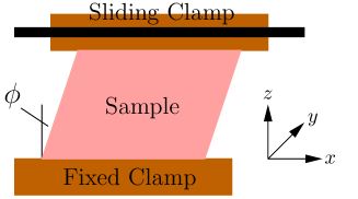
Figure 1: (Color online) Sketch of a slider apparatus where the upper clamp slides on a horizontal bar such that the extension of the sample in the $z$-direction remains fixed.

The second setup, which is depicted in Fig. 2, is one in which opposing surfaces of the sample remain essentially parallel but in which the height of the sample (its extension in the $z$-direction) decreases upon shearing. Hence, the applied shear is, strictly speaking, not just simple shear. In the following we will refer to the this apparatus as a tilt apparatus.

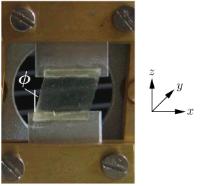
Figure 2: (Color online) One of the two tilt apparatuses used by KF. The photo has been taken from Ref. KramerFinkel2007 .

III.1 Slider apparatus

To make our arguments to follow as concrete and simple as possible, we now choose a specific coordinate system. That is, we choose our $z$ direction along the uniaxial direction $\bm{{\rm n}}_{0}$ of the unsheared samples, $\bm{{\rm n}}_{0}=(0,0,1)$, and we choose our $x$ direction as the direction along which the sample is clamped, which is perpendicular to $\bm{{\rm n}}_{0}$, cf. Fig. 1. With these coordinates, the deformation tensor for both the slider apparatus and the tilt apparatus is of the form

$$\underline{\underline{\Lambda}}=\left(\begin{array}[]{ccc}\Lambda_{xx}&0&\Lambda_{xz}\\ 0&\Lambda_{yy}&0\\ 0&0&\Lambda_{zz}\end{array}\right).$$ (8)

As can be easily checked, for this type of deformation, the layer normal lies along the $z$-direction for the unsheared and for the sheared samples. Thus, the tilt angle $\Theta$ between $\bm{{\rm n}}$ and $\bm{{\rm k}}$ is identical to the tilt angle between $\bm{{\rm n}}$ and the $z$-axis, and we can parametrize the director as

$$\bm{{\rm n}}=(\sin\Theta,0,\cos\Theta)\,.$$ (9)

It is worth noting that a deformation tensor of the form shown in Eq. (8) leads to a particularly simple expression for the semi-soft contribution to $f$, $f_{\rm semi}=(1/2)\alpha\mu\Lambda_{xx}^{2}\sin^{2}\Theta$, which combines with the tilt energy density to $f_{\text{tilt}}+f_{\rm semi}=(1/2)\zeta(\Lambda_{xx})\sin^{2}\Theta$. Thus, as indicated above, our model depends for the experimental geometries under consideration on $\alpha$ and $a_{t}$ through a single effective parameter, viz. $\zeta(\Lambda_{xx})=a_{t}+\Lambda_{xx}^{2}\alpha\mu$.

From the photos of the experimental samples provided in Ref. KramerFinkel2007 , see Figs. 1 and 2, it appears as if $\Lambda_{xx}$ does not deviate significantly from 1. In the following, we set $\Lambda_{xx}=1$ for simplicity footnoteLambdaXX . In this event $\zeta(\Lambda_{xx})=\zeta\equiv a_{t}+\alpha\mu$. In the slider apparatus, the extent of the sample in the $z$-direction is fixed, and hence $\Lambda_{zz}=1$. The incompressibility constraint $\det\underline{\underline{\Lambda}}=1$ thus mandates that $\Lambda_{yy}=1$. The remaining nonzero component of the deformation tensor is entirely determined by the externally imposed shear, $\Lambda_{xz}=\tan\phi$, where $\phi$ is the mechanical tilt angle of the sample, see Fig. 1. The only remaining degree of freedom in the problem is, therefore, the angle $\Theta$.

To calculate $\Theta$ as a function of $\phi$, we insert the just discussed deformation tensor into $f$ and then minimize $f$ over $\Theta$ holding $\phi$ fixed. For $\phi$ small, this can be done analytically by expanding $f$ to harmonic order in $\Theta$ and by then solving the resulting linear equation of state for equilibrium value of $\Theta$. This type of analysis is presented in the appendix. To provide reliable predictions for larger shears, one has to refrain from expanding in $\Theta$ and use numerical methods instead. To this end, we minimize $f$ numerically assuming, based on what we discussed at the end of Sec. II, that $B/\mu=10$ and $\zeta/\mu\in\{0.1,1,5,20\}$. For this minimization, we use Mathematica’s FindMinimum routine. Figure 3 shows the resulting curves for $\Theta$ as a function of $\phi$. The dashed horizontal line in Fig. 3 is a guide to the eye; it corresponds to the angle resolution in the KF experiments which was about $1$ degree kramerPrivate .

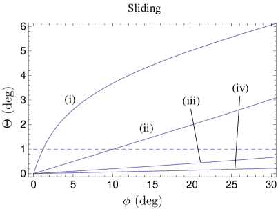
Figure 3: The tilt angle $\Theta$ between the layer normal and the director as a function of the mechanical tilt angle $\phi$ in the slider apparatus for (i) $\zeta/\mu=0.1$, (ii) $\zeta/\mu=1$, (iii) $\zeta/\mu=5$, and (iv) $\zeta/\mu=20$. The dashed line corresponds to the resolution for $\Theta$ in the experiments by KF.

For the slider geometry, the KF data produces clear evidence for the development of Sm$C$-like tilt under simple shear, and our theoretical estimates agree well with the experimental data. However, given that thus far only two data points are available for $\phi>0$, it cannot be judged reliably whether our theoretical curve could be fitted to an experimental curve with more data points. It is encouraging, though, that our curve for $\zeta/\mu=0.1$ agrees with the available experimental points within their errors.

III.2 Tilt apparatus

Now we turn to the tilt geometry. The essential difference between the slider and the tilt geometry is that in the former the height of the sample $L_{z}(\phi)$ remains constant, $L_{z}(\phi)=L_{z}$ ($d_{0}$ times the number of smectic layers) whereas in an ideal tilter, $L_{z}(\phi)$ is not constant but rather decreases as $\phi$ increases, $L_{z}(\phi)=L_{z}\cos\phi$. This difference has far reaching consequences. In the slider, the sample-height remains larger than the modified natural height of the sample created by the director tilt, $L_{z}\cos\Theta$. In other words, the sample is under effective tension. In the tilter, on the other hand, the sample-height $L_{z}\cos\phi$ can be smaller than $L_{z}\cos\Theta$, i.e., the sample can be under effective compression. For a sample under effective $zz$-compression, one has to worry, experimentally and theoretically, about all sorts of complications. Most notable are perhaps buckling and wrinkling.

The theory of buckling of elastic sheets is well established Landau-elas , and we now briefly comment on buckling in the context of the tilt geometry. As mentioned above, a sample clamped into the tilt apparatus can develop a buckling instability, if the height of the sample imposed by tilt, $L_{z}\cos\phi$, is smaller than the natural height of the sample created by the director tilt, $L_{z}\cos\Theta$. As we will see below, our results for $\Theta$ as a function of $\phi$ imply that $\cos\phi<\cos\Theta$, i.e., buckling is possible. Alternatively, this can be seen by calculating the engineering stress $\sigma^{\text{eng}}_{zz}=\partial f/\partial\Lambda_{zz}$, which can be done using the numerical approach outline above. $\sigma^{\text{eng}}_{zz}$ is positive for $\phi>0$ in the slider apparatus, whereas it turns out being negative for $\phi>0$ in the tilt apparatus. Thus, the sample is effectively under tension in the slider apparatus whereas it is effectively under compression in the tilt apparatus, opening the possibility for buckling in the $y$-direction in the latter. The angle $\phi^{c}$ at which buckling sets in is expected to be comparable to that for the well known Euler Strut instability Landau-elas ,

$$\phi^{c}\approx\phi^{\text{Euler}}=\arccos\left[1-\left(\frac{2\,\pi\,L_{y}}{3\,L_{z}}\right)^{2}\right],$$ (10)

where $L_{y}$ is the thickness of the sample in the $y$-direction, and where clamped (rather than hinged) boundary conditions are assumed. A brief derivation of Eq. (10) is given in App. B. In the experiments of KF, $L_{z}=5.0\,\mbox{mm}$ and $L_{y}=0.45\,\mbox{mm}$ kramerPrivate , which leads to $\phi^{\text{Euler}}\approx 15\,\mbox{deg}$. The experimental samples buckle immediately before they rupture kramerPrivate at $\phi=13\,\mbox{deg}$ or $\phi=14\,\mbox{deg}$, which is very close to our estimate for $\phi^{c}$. The observation that buckling occurs immediately before rupturing might suggest that the former actually triggers the latter.

A detailed analysis of sample-wrinkling in the tilt geometry is beyond the scope of the present paper. However, a few comments about wrinkling are in order. The wavelength of wrinkling is expected to be much shorter than that of buckling. Thus, wrinkling can be harder to detect by visual inspection of an experimental sample than buckling, and there is a risk that it remains unnoticed. The main problem is, however, that wrinkling can act as to effectively reduce the mechanical shear in the sample. When designing a tilt experiment, one thus has be very careful to avoid wrinkling. If not, the effects of wrinkling can bias the data, and there is the risk to underestimate the Sm$C$-tilt significantly.

Our calculation of the the Sm$C$-tilt will be for an ideal tilter. Figure 4 shows the tilter of Fig. 2 schematically in a non-tilted and a tilted configuration to make clear that shear and compression are complex in the non-ideal case because the frame-axles allowing angle change are off-set from the corners of the sample.

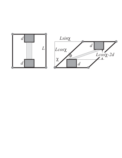
Figure 4: Schematic of shear and compression arising in a non-ideal tilter.

Using elementary trigonometry, one can deduce for the shears and the angle $\phi$

$$\lambda_{xz} = \frac{L}{L-2d}\sin\chi\,,\;\;\;\;\;\lambda_{zz}=\frac{L\cos\chi-2d}{L-2d}\,,$$ (11)

$$\tan\phi = \frac{\tan\chi}{1-(2d/L)\sec\chi}\,,$$ (12)

In particular, the relation between the shear angle $\phi$ and the deformation components $\lambda_{zz}$ and $\lambda_{xz}$ is not simple.

Returning to an ideal tilter, $d=0$, $\chi\equiv\phi$, we calculate the Sm$C$-tilt as a function of the applied mechanical shear, suppressing buckling and wrinkling. Then, the deformation tensor is of the same form (8) as for the slider apparatus, but with the essential difference that here $\Lambda_{xz}=\sin\phi$ and $\Lambda_{zz}=\cos\phi$. As we did for the slider apparatus, we assume $\Lambda_{xx}=1$. The incompressibility constraint then implies that $\Lambda_{yy}=1/\cos\phi$, leaving the angle $\Theta$ as the only degree of freedom. We calculate $\Theta$ as a function of $\phi$ in exactly the same way as above, i.e., we minimize $f$ numerically assuming the values of the model parameters discussed in Sec. II. The resulting curves are shown in Fig. 5.

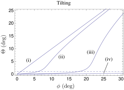
Figure 5: The tilt angle $\Theta$ between the layer normal and the director as a function of the mechanical tilt angle $\phi$ in the tilt apparatus for (i) $\zeta/\mu=0.1$, (ii) $\zeta/\mu=1$, (iii) $\zeta/\mu=5$, and (iv) $\zeta/\mu=20$. The dashed line corresponds to the resolution for $\Theta$ in the experiments by KF.

The dip in Fig. 5 occurs because of a competition between $\zeta$ which would prefer $\Theta=0$ and $B$ which would prefer $\Theta=\phi$. If $\zeta>B$ then it is possible to get curves where $\Theta$ stays close to $0$. The dashed horizontal line in Fig. 5 indicates the angle resolution of about $1$ degree of the KF experiments kramerPrivate .

As mentioned in Sec. III.1, the data points for the slider are compatible with $\zeta/\mu\approx 0.1$. The elastomers used by KF in the slider and the tilter are identical, and, therefore, curve (i) of Fig. 5 should describe the Sm$C$-tilt if the tilter used by KF were ideal or nearly so. Note from Fig. 5, however, that this implies that the Sm$C$-tilt for an ideal tilter at $\phi=13$ or $14\,\mbox{deg}$ should be significantly larger than the experimental resolution, which is incompatible with the findings of Refs. KramerFinkel2007 ; KramerFinkel2008 .

Since any effective compression of the sample along the layer normal, as in a tilter, promotes rather than hampers director rotation, we obtain a Sm$C$-tilt at a given $\phi$ in a tilter if it occurs at the same angle in the slider. It is likely that the failure of KF to observe director rotation in their tilter is due to mechanical instability that effectively reduces the mechanical shear of the sample and thus leads to a systematic suppression of the Sm$C$-tilt in the tilt geometry.

IV Discussion and concluding remarks

In summary, we have developed a neo-classical model for smectic elastomers, and we used this model to study Sm$A$ elastomers under shear in the plane containing the director and the layer normal. In particular, we investigated the tilt angle $\Theta$ between the layer normal and the director for two different experimental setups as a function of the mechanical tilt angle $\phi$ measuring the imposed shear.

Our model builds upon the neo-classical model for smectic elastomers by AW. In their original work, AW chose not to consider the possibility of Sm$C$ order in their theory: they forced the layer normal and the nematic director to be parallel. In our present theory, the fundamental tenet is different in that the nematic director $\bm{{\rm n}}$ and the deformation tensor $\underline{\underline{\Lambda}}$ are independent quantities that must be allowed to seek their equilibrium in the presence of imposed strains or stresses. The layer normal $\bm{{\rm k}}$ is determined entirely by $\underline{\underline{\Lambda}}$. Thus, $\bm{{\rm n}}$ and $\bm{{\rm k}}$ are independent variables that rotate to minimize the free energy - they are not locked together.

In the present paper, we have for simplicity focused on idealized monodomain samples. Boundary conditions in real experiments prevent this simple scenario and produce a microstructure structure of the type that AW discuss in Ref. adams_warner_2005 based on their original model that prohibits Sm$C$ ordering. Our current theory, which admits Sm$C$ ordering, predicts the same type of microstructure; stretching will produce a polydomain layer structure just as the AW theory does. In particular, the existence of Sm$C$ ordering does not contradict the appearance of optical cloudiness. To avoid undue repetition, we refrain discussing this here in more detail and refer the reader to Ref. adams_warner_2005 .

The main finding of our present work is that the tilt angle $\Theta$ between $\bm{{\rm n}}$ and $\bm{{\rm k}}$ is non-zero if a shear in the plane containing $\bm{{\rm k}}$ is imposed. This angle depends on material parameters, the experimental setup, and the magnitude of the imposed shear. Figures 3 and 5 depict our results for the slider apparatus and the tilt apparatus used by KF. As expected, in both setups the angle $\Theta$ decreases as the value of the parameter $\zeta/\mu$ increases, at fixed $\phi$. This is because the director is becoming more strongly anchored to the layer normal. If one keeps $\zeta/\mu$ fixed and varies $B/\mu$ instead, then for $B/\mu\to\infty$ $\Theta$ approaches $\phi$ because in this limit $f_{\text{layer}}$ locks $\Theta$ to $\Theta=\phi$. As $B/\mu$ is decreased then $\Theta$ decreases at fixed $\phi$, because the $f_{\mathrm{tilt}}$ term starts to compete with the $f_{\mathrm{layer}}$ term. In the opposite limit of very small $B/\mu$, $\Theta$ is locked to $\Theta=0$ by virtue of the tilt and semi-soft contributions to $f$. We refrain to show the corresponding curves, which are similar to those depicted in Figs. 3 and 5, to save space. The main difference between our results for the two setups is that for $B>\zeta$ and large $\phi$, say $40$ degrees or so, $\Theta$ is roughly one order of magnitude smaller than $\phi$ in the slider apparatus, whereas it is of the order of $\phi$ in the tilt apparatus.

In closing, we would like to stress once more that the experiment using the slider geometry produces clear evidence of the development of Sm$C$-like tilt under shear as predicted originally in Ref. StenLubSmA2007 . Our theory developed here allowed us to understand in some detail how the magnitude of this tilt depends on the shear geometry and on model/material parameters, such as $\zeta$, which can be reasonably estimated from nematic analogues. Given these estimates, the resulting estimates for the tilt angle vary over a range from being small enough to be essentially unobservable with the X-ray equipment used by the Freiburg group to exceeding the experimental resolution. While the latter is consistent with the shear experiments in the slider geometry, the former is consistent with the stretching experiments by Nishikawa and Finkelmann in which no Sm$C$-like tilt was detected. We believe that the reason for the discrepancy between the rotations in the slider and tilter apparatus lies in a possible wrinkling of the samples in the tilt apparatus used by KF. Mechanical instability leads to an effective reduction of the mechanical shear of the sample causing a systematic underestimation of the Sm$C$-like tilt in the tilt geometry.

Another experimental approach that could be used, at least in principle, to investigate $\Theta$ is to measure changes in the layer spacing, as was done by Nishikawa and Finkelmann nishikawa_finkelmann_99 . It should be noted, however, that in this approach one measures $\cos\Theta$ rather than $\Theta$ directly. For small values of Sm$C$ tilt, say $\Theta=1$ degree, $\cos\Theta\approx 0.9998$ which is practically indistinguishable from the $\cos\Theta=1$ pertaining to Sm$A$ order.

For a refined comparison between experiment and theory it would be useful to critically evaluate and potentially improve the design of the tilt apparatuses regarding sample-wrinkling. Also, it would be interesting to perform shear and stretching experiments with an angle resolution better than $1\,\mbox{deg}$. We hope that our work stimulates the interest for such experiments.

Appendix A Analytical consideration for small angles

For arbitrary Sm$C$-tilt angle $\Theta$, the total elastic energy density $f$ is, for the deformations discussed in Sec. III, a fairly complicated conglomerate of trigonometric functions (and powers thereof) of $\Theta$ and $\phi$. Thus, we resorted in Sec. III to a numerical approach to determine the equilibrium value of $\Theta$ over a wide range of the imposed mechanical tilt angle $\phi$. Here, we focus on the regime of $\phi$ where $\Theta$ is small, such that it is justified to expand $f$ to harmonic order in $\Theta$. In this case, the equations of state are linear in $\Theta$, of course, and are therefore readily solved. For the slider apparatus we obtain

$$\Theta=\frac{(r-1)r\mu\tan\phi}{r\zeta+\mu(1-r)[1-r+r\tan^{2}\phi]}\,,$$ (13)

and for the tilt apparatus we get

$$\Theta=\frac{2^{-1}(r-1)r\mu\sin 2\phi}{r\zeta-rB\sin^{2}2\phi+\mu(1-r)[1-r\cos 2\phi]}\,.$$ (14)

Equations (13) and (14) imply, that the Sm$C$-tilt in both setups is identical for small $\phi$,

$$\Theta=\frac{(r-1)r\mu\,\phi}{r\zeta+\mu(1-r)^{2}}+O(\phi^{3})\,.$$ (15)

This is consistent with Figs. 3 and 5, where the initial slopes are identical for identical values of $\zeta$ (though this is perhaps somewhat hard to see because the ordinate-scales are different in the two figures).

An interesting related question, which we have not addressed in the main text because there is currently no experimental data available, is that of the stress that is caused by the imposed shear strains. From the above, it is straightforward to calculate this stress for small $\phi$. Inserting Eq. (15) into the aforementioned harmonic (in $\Theta$) total elastic energy density provides us with an effective $f$ in terms of $\phi$. From this effective $f$, we readily extract the engineering or first Piola-Kirchhoff stress as

$$\sigma^{\text{eng}}_{xz}=\frac{\partial f}{\partial\Lambda_{xz}}=\frac{r^{2}\mu\zeta\,\phi}{r\zeta+\mu(1-r)^{2}}+O(\phi^{3})\,.$$ (16)

Equation (16) highlights a problem that arises when the tilt and the semi-soft contributions $f_{\text{tilt}}$ and $f_{\text{semi}}$ to the total elastic energy density are missing, and one allows $\bm{{\rm n}}$ and $\underline{\underline{\Lambda}}$ to be independent quantities. Setting $\zeta=0$ in Eq. (16) leads to zero stress for non-zero $\phi$, i.e., this truncated model predicts soft elasticity. This soft elasticity, however, is not compatible with Sm$A$ elastomers crosslinked in the Sm$A$ phase, such as the experimental samples of Refs. nishikawa_finkelmann_99 ; KramerFinkel2007 , where the anisotropy direction is permanently frozen into the system.

Appendix B Euler instability in the tilt apparatus

In this appendix, we give a brief derivation of Eq. (10). We are interested primarily in a rough estimate for $\phi^{c}$, and therefore, for simplicity, we assume that we can ignore the effects of smectic layering. In the following, we employ, for convenience, the Lagrangian formulation of elasticity theory.

In the Lagrangian formulation, the elastic energy density of a thin elastomeric film with thickness $L_{y}$ and height $L_{z}$ that is compressed along the $z$-direction can be written as

$$f_{\text{film}}=\textstyle{\frac{1}{2}}\,\kappa\left(\partial^{2}_{z}u_{y}\right)^{2}+\textstyle{\frac{1}{2}}\,Y_{2d}u_{zz}^{2}\,,$$ (17)

where the choice of coordinates is the same as depicted in Fig. 2. $u_{y}$ is the $y$-component of the elastic displacement $\bm{{\rm u}}=\bm{{\rm R}}-\bm{{\rm x}}$, and $u_{zz}^{2}$ is the $zz$-component of the Cauchy-Saint-Venant strain tensor, $u_{ij}=\frac{1}{2}(\partial_{i}u_{j}+\partial_{j}u_{i}+\partial_{i}u_{k}\partial_{j}u_{k})$. $\kappa$ and $Y_{2d}$ are, respectively, the bending modulus and Young’s modulus of the film, which are given in the incompressible limit by $\kappa=(\mu/3)L_{y}^{3}$ and $Y_{2d}=3\mu L_{y}$ Landau-elas . At leading order, $\partial_{z}u_{z}=-|\delta L_{z}/L_{z}|$, where we have used that the height change $\delta L_{z}$ is negative when the sample is effectively compressed as in the tilt apparatus. This leads to

$$u_{zz}=-|\delta L_{z}/L_{z}|+\textstyle{\frac{1}{2}}\,(\partial_{z}u_{y})^{2},$$ (18)

when we concentrate on the parts of $u_{zz}$ that are most important with respect to buckling in the $y$-direction. Next, we substitute the strain (18) into Eq. (17) and switch to Fourier space. To leading order in the elastic displacement, this produces

$$\tilde{f}_{\text{film}}=\frac{1}{2}\left\{\kappa\,q_{z}^{2}-Y_{2d}\,\left|\frac{\delta L_{z}}{L_{z}}\right|\right\}q_{z}^{2}\,\tilde{u}_{y}(\bm{{\rm q}})\tilde{u}_{y}(-\bm{{\rm q}})\,,$$ (19)

where $\bm{{\rm q}}$ is the wavevector conjugate to $\bm{{\rm x}}$, $\tilde{u}_{y}$ is the Fourier transform of $u_{y}$, and so on. Equation (19) makes it transparent that buckling occurs for

$$\left|\frac{\delta L_{z}}{L_{z}}\right|=\frac{\kappa}{Y_{2d}}\,q_{z}^{2}=\frac{L_{y}^{2}}{9}\,q_{z}^{2}\,.$$ (20)

The smallest value of $q_{z}$ is determined by the specifics of the boundary conditions. From Fig. 2 it appears as if the sample of KF is clamped such that it prefers to stay parallel to the clamps in their immediate vicinity. In this case, the smallest value of $q_{z}$ is $q_{z}=2\pi/L_{z}$. For hinged boundary conditions, in comparison, its smallest value would be $q_{z}=\pi/L_{z}$. Using the former value and exploiting that, approximately, $|\delta L_{z}/L_{z}|=1-\cos\phi$, we obtain the estimate (10) for the onset of the Euler instability in the tilt apparatus.

References

- (1) For a review on liquid crystal elastomers see M. Warner and E.M. Terentjev, Liquid Crystal Elastomers (Clarendon Press, Oxford, 2003).
- (2) For a review see P. G. de Gennes and J. Prost, The Physics of Liquid Crystals (Clarendon Press, Oxford, 1993); S. Chandrasekhar, Liquid Crystals (Cambridge University Press, Cambridge, 1992).
- (3) E. Nishikawa and H. Finkelmann, Macromol. Chem. Phys. 200, 312 (1999).
- (4) J. M. Adams and M. Warner, Phys. Rev. E 71, 021708 (2005).
- (5) O. Stenull and T. C. Lubensky, Phys. Rev. E 76, 011706 (2007).
- (6) D. Kramer and H. Finkelmann, arXiv:0708.2024.
- (7) D. Kramer and H. Finkelmann, Phys. Rev. E 78, 021704 (2008).
- (8) P. Bladon, E. Terentjev, and M. Warner, J. Phys. II (France) 4, 75 (1994).
- (9) L. R. G. Treloar, The Physics of Rubber Elasticity (Clarendon Press, Oxford, 1975).
- (10) Note that the layer compression term formulated by AW is of the form whereas setting in Eq. (3) produces . This form is chosen for consistency with the Chen-Lubensky model of smectics. This term can be factorized into for . Thus the difference is merely factor of in the definition of the smectic modulus in the two representations.
- (11) M. Brehmer, R. Zentel, F. Gieselmann, R. Germer, and P. Zungenmaier, Liquid Crystals 21, 589 (1996).
- (12) P. Archer and I. Dierking, Phys. Rev. E 72, 041713 (2005).
- (13) E. M. Terentjev, M. Warner, R. B. Meyer, and J. Yamamoto, Phys. Rev. E 60, 1872 (1999).
- (14) H. Finkelmann, I. Kundler, E. M. Terentjev, and M. Warner, J. Phys. II (France) 7, 1059 (1997).
- (15) We checked the validity of this assumption by allowing to relax to its equilibrium value, i.e., we repeated our analysis using the that minimizes rather than . The results obtained by using this more involved approach do not differ significantly from those obtained our simplified approach with .
- (16) D. Kramer and H. Finkelmann, private communication.
- (17) L.D. Landau and E.M. Lifshitz, Theory of Elasticity, 3rd Edition (Pergamon Press, New York, 1986).