REGULAR AND CHAOTIC MOTION IN ELLIPTICAL GALAXIES

Abstract

Here I review recent work, by other authors and by myself, on some particular topics related to the regular and chaotic motion in elliptical galaxies. I show that it is quite possible to build highly stable triaxial stellar systems that include large fractions of chaotic orbits and that partially and fully chaotic orbits fill different regions of space, so that it is important not to group them together under the single denomination of chaotic orbits. Partially chaotic orbits should not be confused with weakly fully chaotic orbits either, and their spatial distributions are also different. Slow figure rotation (i.e., rotation in systems with zero angular momentum) seems to be always present in highly flattened models that result from cold collapses, with the rotational velocity diminishing or becoming negligibly small for less flattened models. Finally, I comment on the usefulness and limitations of the classification of regular orbits via frequency analysis.

1 Introduction

It is fitting, in this conference in memory of N. Voglis, to recall that I became interested in the investigation of regular and chaotic motions in elliptical galaxies thanks to a paper of his VKS02 . By that time, I had been working on N–body problems for two decades, and on regular and chaotic motion for seven or eight years, but I had never been involved in research on elliptical galaxies. The paper by Voglis and his coworkers showed me that, with the computers and the numerical tools I had at my disposal, I might be able to contribute significantly to a very interesting subject and, in fact, I have been devoted to that subject ever since.

Having worked in this field for a few years only, it would be presumtuous from my part to attempt to present here a complete review of the subject. Alternatively, to be a relative newcomer to the field has the advantage of bringing to it views and opinions different from the prevailing ones: they may be wrong, but they stimulate progress.

Therefore, I will limit the scope of this review to a few items that have been of particular interest to me and which I have strived to clarify with my research: 1) Can we build stable triaxial models of stellar systems that contain high fractions of chaotic orbits?; 2) Is the distinction between partially and fully chaotic orbits of any use?; 3) Is figure rotation significant in triaxial stellar systems?; 4) Which are the usefulness and limitations of frequency analysis for the classification of large numbers of regular orbits in model stellar systems?

Since galactic dynamics is not the only subject of this conference, which includes other fields like celestial mechanics, it may be useful to recall that the time scales pertinent to galaxies are completely different from those that rule the Solar System. While the age of the latter is of the order of $10^{8}$ orbital periods, galactic ages are of the order of $10^{2}$ orbital periods only. Thus, the chaotic orbits we will refer here are much more strongly chaotic (i.e., their Lyapunov times measured in orbital periods are much shorter) than those of the Solar System. Technical tools, such as frequency analysis, should also be considered with this fact in mind.

2 Highly chaotic triaxial stellar systems

2.1 Building self–consistent triaxial stellar systems

A popular method to build a self–consistent triaxial stellar system is the one due to Schwarzschild Sch79 . One chooses a density distribution and obtains the potential that it creates; a library of thousands of orbits is then computed in that potential and weights are assigned according to the time that a body on that orbit spends in different regions of space; finally, those weights are used to compute the relative numbers of those orbits that are needed to obtain the original density distribution.

Another way to proceed is to use an N–body code to build a triaxial stellar system (e.g., through the collapse of an N–body system initially out of equilibrium), then to smooth and to freeze the potential fitting it with adequate formulae, to use these formulae, together with the positions and velocities of the bodies as initial conditions, to compute a representative sample of orbits in that potential and, finally, to classify those orbits to get the orbital structure of the system VKS02 .

Those two methods should be regarded as complementary. Schwarzschild’s one allows a very precise definition of the density distribution of the system one wants to study; alternatively, some properties of the models dictated by mathematical simplicity (e.g., constant axial ratios over the whole system) might bias its results, while the N–body method is free of that problem.

2.2 The problem of chaotic orbits in Schwarzschild’s method

Schwarzschild Sch93 found it necessary to include chaotic orbits in his models but, then, these were not fully stable. He built several models using orbits computed over a Hubble time and, subsequently, followed those orbits for two additional Hubble times. When he computed the axial ratios obtained using the data for the third Hubble time, he found significant differences with respect to the ratios computed over the first Hubble time, from a low of about 4% for his second and fourth models, to a high of about 17% for his fifth model.

The cause of that evolution is that chaotic orbits change their behaviour with time, resembling that of regular orbits at certain intervals, behaving more chaotically at other intervals and exploring different regions of space in the meantime. Moreover, that weaker or stronger chaotic behaviour can be traced with Lyapunov exponents computed over finite intervals which decrease and increase their values accordingly KM94 , Muz07 . Merritt and his coworkers tried to solve this problem using what they called ”fully mixed solutions” MF96 and, more recently, integrating orbits over five Hubble times Cap07 . In the former work, they found solutions for the weak cusp model, but not for their strong cusp model; the subsequent evolution of these models to test their stability was not investigated, however. In the latter work they indicate that there is ”a slight evolution toward a more prolate shape”, but they provide no quantitative estimates other than indicating that differences in velocity dispersions are ”almost always below 10%”. Clearly, it is very difficult to incorporate chaotic orbits in Schwarzschild’s method: as some chaotic orbits begin to behave more chaotically, one needs to have other chaotic orbits that behave more regularly as compensation; such a delicate equilibrium cannot be attained simply obtaining the weights of chaotic orbits over longer integration times and, moreover, the relatively low number of orbits used (typically a few thousands) makes even more difficult that task. Finally, the usual imposition of constant axial ratios over the whole system in Schwarzschild’s method prevents the existence of a rounder halo of chaotic orbits that seems to be a necessary condition to have highly chaotic triaxial stellar systems VKS02 , MCW05 , AMNZ07 .

2.3 The stability of highly chaotic triaxial stellar systems

The models of the N–body method are built self–consistently from the start and typically contain hundreds of thousands, or even millions, of bodies so that they should be free of the difficulties that plage the construction of highly chaotic triaxial stellar systems with Schwarzschild’s method. In fact, stable models with high fractions of chaotic orbits were obtained with the N-body method, using about $10^{5}$ particles VKS02 , MCW05 ; moreover, the fractions of the different types of orbits were not significantly altered when the potential was fitted to the N–body distribution at different times. A stable cuspy model that was mildly triaxial and made up of 512,000 particles, plus several others with 128,000 particles, were also built HB01 ; later on, it was shown that the introduction of a black hole, although affecting the inner regions of the model, did not alter the triaxiality at larger radii and the authors concluded that the triaxiality of elliptical galaxies is not inconsistent with the presence of supermassive black holes at their centers HB02 .

Highly stable models of $10^{6}$ particles were built by us with the N–body method AMNZ07 , MNZ08 : all of them have decreasing flattening from center to border, which arised naturally from the N–body evolution during the generation of the systems; they have different degrees of flattening and triaxiality, two of them are moderately cuspy ($\gamma\approx 1.0$), and all have high fractions (between 36% and 71%) of chaotic orbits. When integrated with the N–body code, our models suffer changes in their central density and minor semiaxis values which do not exceed, respectively, about 4% and 2% over a Hubble time. Nevertheless, these changes are most likely due to collisional effects of the N–body code HB90 because, when the number of bodies is reduced by a factor of 10 (and their masses are increased by the same factor), those changes increase by factors between 3 and 10. Alternatively, integrating the motion of the bodies in the fixed smooth potential, which suppresses the collisional effects (and which, by the way, is what Schwarzschild did) reduces those changes to 0.1% only (i.e., between one and two orders of magnitude smaller than those found by Schwarzchild Sch93 ).

Thus, we may conclude that highly stable triaxial models with large fractions of chaotic orbits can be built with the N–body method. The difficulties to build such models with Schwarzschild’s method should thus be attributed to the method itself and not to physical reasons.

3 Partially and fully chaotic orbits

Since we are dealing with stationary systems, the orbits of the particles that make them up obey the energy integral, but they need two additional isolating integrals to be regular orbits. Thus, we distinguish between partially chaotic orbits (one additional integral besides energy) and fully chaotic orbits (energy is the only integral they obey). A practical way to make the distinction is to compute the six Lyapunov exponents: they come in three pairs of equal value and opposite signs, due to the conservation of phase space volume, and each isolating integral makes zero one pair. Thus, in our case, two Lyapunov exponents are always zero (due to energy conservation); of the remaining four, if two are positive the orbit is fully chaotic, if only one is positive the orbit is partially chaotic and, finally, if all are zero the orbit is regular.

It was noted in PV84 that orbits obeying two isolating integrals have smaller fractal dimension than orbits obeying only one, but earlier hints of the differences between them can also be found in GS81 (whose semi-stochastic orbits are probably what we now call partially chaotic orbits) and in CGG78 (whose orbits in their big and small seas can be identified, respectively, with the fully and partially chaotic orbits).

The reason why distinguishing partially from fully chaotic orbits in galactic dynamics is important is that, since they obey different numbers of isolating integrals, they have different spatial distributions as shown in Muz03 , MM04 , MCW05 , AMNZ07 and MNZ08 . In triaxial systems, partially chaotic orbits usually exhibit a distribution intermediate between those of regular and of fully chaotic orbits, and a possible explanation is that some of the partially chaotic orbits lie in the stochastic layer surrounding the resonances and thus behave similarly to regular orbits NPM07 . Nevertheless, that is not the whole story as some partially chaotic orbits seem to obey a global integral, rather than local ones AMNZ07 .

Partially chaotic orbits should not be confused with fully chaotic orbits with low Lyapunov exponents, which also tend to have distributions more similar to those of regular orbits than those of fully chaotic orbits with high Lyapunov exponents MM04 , MCW05 . It is worth recalling that, no matter how small their Lyapunov exponents are, fully chaotic orbits obey only one isolating integral while partially chaotic orbits obey two so that, from a theoretical point of view, they are indeed different kinds of orbits. From a practical point of view, it is also easy to see that they have different distributions: Table 1 gives the axial ratios of the distributions of different kinds of orbits for models E4, E5 and E6 from AMNZ07 and E4c and E6c from MNZ08 ; the x, y and z axes are parallel, respectively, to the major, intermediate and minor axes of the models. The third column gives the axial ratios for the distributions of partially chaotic orbits, and the fourth and fifth columns give the same ratios for weakly fully chaotic orbits for two choices of the limiting value of the Lyapunov exponents used to define ”weakly”, 0.050 and 0.100. Although for some models (e.g. E4 and E4c) the possible differences are masked by the rather large statistical errors, it is clear from the Table that the distributions of partially chaotic orbits are significantly different from those of weakly fully chaotic orbits (at the $3\sigma$ level) for the other models.

Table 1: Axial ratios of the different classes of orbits in our models.

Ratio	System	Partially Ch.	W.F.Ch. (0.050)	W.F.Ch. (0.100)
y/x	E4	$0.896\pm 0.064$	$0.692\pm 0.027$	$0.745\pm 0.019$
	E5	$0.808\pm 0.036$	$0.764\pm 0.024$	$0.797\pm 0.017$
	E6	$0.658\pm 0.035$	$0.789\pm 0.027$	$0.845\pm 0.019$
	E4c	$0.748\pm 0.027$	$0.733\pm 0.016$	$0.730\pm 0.013$
	E6c	$0.528\pm 0.020$	$0.693\pm 0.013$	$0.700\pm 0.010$
z/x	E4	$0.790\pm 0.054$	$0.802\pm 0.035$	$0.826\pm 0.024$
	E5	$0.477\pm 0.018$	$0.684\pm 0.021$	$0.708\pm 0.014$
	E6	$0.286\pm 0.013$	$0.644\pm 0.022$	$0.673\pm 0.015$
	E4c	$0.692\pm 0.024$	$0.762\pm 0.017$	$0.757\pm 0.013$
	E6c	$0.334\pm 0.010$	$0.466\pm 0.007$	$0.490\pm 0.006$

At any rate, it is clear that the distributions of partially and fully chaotic orbits differ significantly and that they should not be bunched together as a single group of chaotic orbits. The problem is that the computation of the Lyapunov exponents demands long computation times and there are not yet faster methods that allow to distinguish partially from fully chaotic orbits. The fact that many chaotic orbits can be frequency analyzed and are found to lie in regions of the frequency map corresponding to regular orbits KV05 might, perhaps, lead to a faster method of separation in the future. Nevertheless, many fully chaotic orbits can be frequency analyzed, while many partially chaotic orbits cannot AMNZ07 , so that much remains to be done before a workable method based on frequency analysis can be designed.

4 Figure rotation in triaxial systems

Although the system investigated in MCW05 had been regarded as stationary, integrations much longer than those used in that work revealed that, in fact, it was very slowly rotating around its minor axis Muz06 . The total angular momentum of the system was zero, so that this was an unequivocal case of figure rotation.

Figure rotation was also found in most of the models studied in AMNZ07 and MNZ08 and it is clear that the rotational velocity increases with the flattening of the system; only model E4 from AMNZ07 , which is almost axially symmetric, prolate and with axial ratio close to 0.6 has no significant rotation. It should be stressed, however, that even the highest rotational velocities found thus far are extremely low: the systems can complete only a fraction of a revolution in a Hubble time or, put in a different way, the radii of the Lindblad and corotation resonances are at least an order of magnitude larger than the systems themselves.

It had been suggested that figure rotation might produce important changes in the degree of chaoticity MF96 and it turned out that, in spite of the extremely low rotational velocity, a significant difference in the fraction of chaotic orbits was found between the models of MCW05 and Muz06 which only differ in that the former is stationary and the latter is rotating. Alternatively, no significant difference was found for the different kinds of regular orbits in those two models. The most likely explanation is that, although the rotational velocity is too low to produce a measurable effect on the regular orbits, the break of symmetry caused by the presence of rotation suffices to increase chaos significantly.

5 Musings on orbital classification through frequency analysis

5.1 Classification methods

The spectral properties of galactic orbits were investigated by Binney and Spergel BS82 and, more recently, Papaphilippou and Laskar PL96 and PL98 applied to stellar systems the frequency analysis techniques developed by the latter for celestial mechanics. Following the ideas of Binney and Spergel, Carpintero and Aguilar CA98 developed an automatic orbit classification code. Kalapotharakos and Voglis KV05 developed a classification system based on the frequency map of Laskar and, later on, I Muz06 improved it somewhat.

Having used extensively both the Carpintero and Aguilar CMW99 , MCW00 , CVM01 , CMVW03 and MCW05 , and the Kalapotharakos and Voglis methods Muz06 , AMNZ07 and MNZ08 , I strongly prefer the latter. The main advantage of the Kalapotharakos and Voglis method is that one can see what is happening throughout the process. It is very easy to detect problems from the anomalous positions that the corresponding frequency ratios yield on the frequency map and, thus, to improve the method. This is an aspect that deserves to be emphasized: the need to use frequencies different from those corresponding to the maximum amplitudes had not been noted in KV05 , but it was in Muz06 , probably because a somewhat cuspier potential was investigated in the latter work; similarly, that distinction was unnecessary for the long axis tubes (LATs hereafter) of Muz06 , but had to be made for those of the almost axially symmetric E4 system of AMNZ07 . In other words, as one explores different stellar system models (cuspier, closer to axisymmetry, and so on) the orbital classification system may need to be improved and that need is quite evident with the Kalapotharakos and Voglis method. Thanks to these improvements, virtually all the regular orbits can be classified with the frequency map, while usually between 10% and 15% of them remain unclassified with the other method MCW05 and J05 .

Besides, separation of chaotic from regular orbits with the method of Carpintero and Aguilar is erratic, at least in rotating systems CMVW03 . Since the problem seems to arise from the presence of nearby lines in the spectra, which is worse in rotating systems but not exclusive of them, I strongly suspect that orbit classification in non–rotating systems may also be affected. That is why in our last work with that method MCW05 we used it only to classify regular orbits, previously selected using Lyapunov exponents.

5.2 Which frequency to choose?

Frequency analysis is usually performed on complex variables formed taking one coordinate as the real part and the corresponding velocity as the imaginary part. One thus gets the frequencies Fx, Fy and Fz corresponding, respectively, to motion along the (x, y, z) axes which, in turn, are parallel to the main axes of the stellar system. The frequencies usually selected for the frequency map are those corresponding to the maximum amplitudes in each coordinate WFM98 , KV05 , but it has been known since 1982 BS82 that, due to a libration effect, one should not always take those. Besides, another effect linked to very highly elongated orbits also demands to adopt frequencies which are not the ones corresponding to the maximum amplitudes Muz06 , AMNZ07 . Nevertheless, it is just fair to note that these exceptions are not too common: out of 17,103 orbits investigated in AMNZ07 and MNZ08 only 265 (1.5%) needed the former correction and 153 (0.9%) the latter one. These fractions vary considerably from one model to another, however, and as the affected orbits tend to concentrate at low absolute values of energy and/or are extremely elongated, not taking these effects into account might bias the sample of classified orbits.

5.3 The usefulness of the energy vs. frequency plane

Regular orbits obey two additional isolating integrals, besides energy, and the values of the orbital frequencies are related to these integrals. For a given energy, different frequencies imply different values of the other integrals and, thus, different types of orbits. Inner and outer LATs, short axis tubes, boxes and even different resonant orbits can be separated on the energy vs. frequency (or frequency ratio) plane, but that does not mean that it is practical to use it, because those separations are more easily done on the frequency map.

Nevertheless, some insight can be gained from the use of the energy vs. frequency plane. Figure 1 of Muz06 offers a good example, because that plane was used there to show that one should not always use the frequency corresponding to the maximum amplitude as the principal frequency. Besides, while in KV05 it was correctly stated that outer LATs had larger Fx/Fz values than inner LATs, no indication of which was the separating value was provided there. Actually, as shown in Figure 2 of AMNZ07 , one has to use the energy vs. frequency ratio plane to separate inner from outer LATs, because the separating value varies with the energy of the orbit.

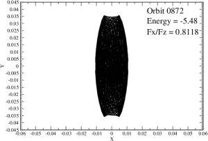
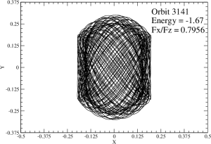
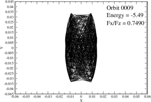
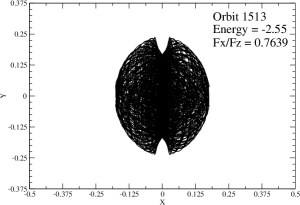
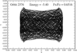
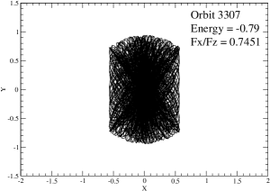
Figure 1: Projection on the (x, y) plane of several examples of LATs; see text for details

Figure 1 presents the (x, y) projections of several LATs from model E4 of AMNZ07 . The orbits on the left column have similar energy values, close to the minimum energy of -5.96 and, although their Fx/Fz values range from 0.6516 to 0.8118, they are all inner LATs, as evidenced by their concave upper and lower limits. We also notice that their extension along the x axis is reduced as their Fx/Fz values increase and, in fact, the regions of space occupied by orbits 0872 and 0009 resemble more those occupied by outer LATs than those occupied by inner LATs. We found a similar effect on the x extension of the orbits at other energy values although, when the separation shown in Figure 2 of AMNZ07 is crossed, there is also of course a change from inner to outer LATs. The upper and middle parts of the right column of Figure 1 correspond to orbits 3141 and 1513 that are virtually face to face at each side of the separation on the energy vs. frequency ratio plot: they have similar Fx/Fz values but, due to their energy difference, the former is an outer, and the latter an inner, LAT. Notice also that the Fx/Fz value of (outer LAT) orbit 3141 is lower than that of (inner LAT) orbit 0872. Finally, the lower right section of Figure 1 corresponds to (outer LAT) orbit 3307, whose Fx/Fz value is lower than those of (inner LAT) orbits 0009 and 0872.

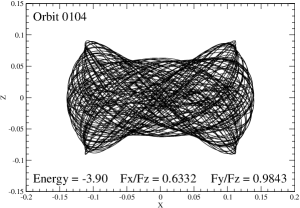
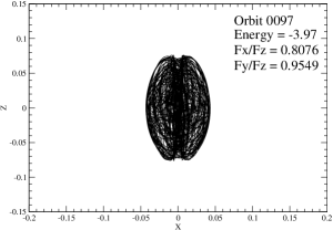
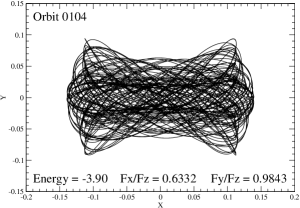
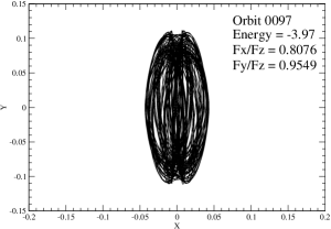
Figure 2: Projection on the (x, y) plane of two examples of boxes; see text for details

Interestingly, the shortening of the x axis as the Fx/Fz ratio increases, shown above for the LATs, affects the boxes as well. Figure 2 presents the (x, y) and (x, z) projections of orbits 0104 and 0097 from model E4 of AMNZ07 , which have both essentially the same energy. Nevertheless, while the former, with Fx/Fz = 0.6332, lies straight on the line occupied by the boxes on the energy vs. frequency ratio plane, the latter, with Fx/Fz = 0.8076, lies well above that line. We see on the left part of Figure 2 that 0104 is indeed a typical box, but the right part shows that 0097, although still a box, is strongly compressed along the x axis.

Due to their elongation along the major axis, inner LATs and boxes are usually considered as the main building blocks of highly elongated triaxial systems, but we now see that there are inner LATs and boxes that are, in fact, strongly compressed along that axis. To put things in the proper perspective we should emphasize, however, that these orbits were found in the almost rotationally symmetric model E4 of AMNZ07 and that they are not very abundant.

6 Discussion

We have reviewed several papers on triaxial stellar systems built with the N–body method that show that it is perfectly possible to have strongly chaotic triaxial stellar systems that are also highly stable over periods of the order of a Hubble time. The difficulties to build such systems with Schwarzschild’s method should thus be attributed to the method itself and not to physical reasons.

It is clear, both from a theoretical and from a practical point of view, that partially and fully chaotic orbits populate different regions of space and should not be bunched together under the single banner of chaotic orbits. The main problem here is that the single method thus far available to separate them, that of Lyapunov exponents, is very slow and faster methods are wanted. We also showed that the distribution of partially chaotic orbits is different from that of weakly fully chaotic orbits, in accordance with the fact that the former obey two isolating integrals of motion and the latter only one.

Very slow figure rotation seems to be an ordinary trait of strongly elongated triaxial stellar models formed through the collapse of cold N–body systems. The rotational velocity diminishes, and even disappears entirely, as one goes to less elongated and less triaxial models.

Frequency analysis offers a very useful tool for the classification of large numbers of regular orbits. I strongly favor the use of the method of Kalapotharakos and Voglis KV05 , with the improvements we introduced in Muz06 and AMNZ07 . Since the need for those improvements became apparent when models with different characteristics (cuspiness, approximate rotational symmetry) were considered, it would not be surprising that further refinements will be necessary as the method is applied to other systems. Nevertheless, a nice feature of this method is that, when there is such need, it becomes plainly evident. Besides, plots of known integrals, such as energy, and the orbital frequencies (or frequency ratios), that are related to the values of the integrals, are very useful to reveal peculiarities of the orbits as one explores different models; a good example of this is provided by the compression along the major axis of some LATs and boxes from an almost axisymmetric system, shown in our Figures 1 and 2.

7 Acknowledgements

I am very grateful to Héctor R. Viturro and to Ruben E. Martínez for their technical assistance, and to Lilia P. Bassino and to an anonimous referee for carefully reading the first version of this paper and suggesting some language improvements. This work was supported with grants from the Consejo Nacional de Investigaciones Científicas y Técnicas de la República Argentina, the Agencia Nacional de Promoción Científica y Tecnológica and the Universidad Nacional de La Plata.

References

- (1) R.O. Aquilano, J.C. Muzzio, H.D. Navone and A.F. Zorzi: Celest. Mech. Dynam. Astron., Vol.99, 307 (2007)
- (2) J. Binney and D. Spergel: Astrophys. J., Vol.252, 308 (1982)
- (3) R. Capuzzo-Dolcetta, L. Leccese, D. Merritt and A. Vicari, Astrophys. J., Vol.666, 165 (2007)
- (4) D.D. Carpintero and L.A. Aguilar: MNRAS, Vol.298, 1 (1998)
- (5) D.D. Carpintero, J.C. Muzzio, M.M. Vergne and F.C. Wachlin: Celest. Mech. Dynam. Astron., Vol.85, 247 (2003)
- (6) D.D. Carpintero, J.C. Muzzio, and F.C. Wachlin: Celest. Mech. Dynam. Astron., Vol.73, 159 (1999)
- (7) G. Contopoulos, L. Galgani and A. Giorgilli: Phys. Rev. A, Vol.18, 1183 (1978)
- (8) S.A. Cora, M.M. Vergne and J.C. Muzzio: Astrophys. J., Vol.546, 165 (2001)
- (9) J. Goodman and M. Schwarzschild: Astrophys. J., Vol.245, 1087 (1981)
- (10) Hernquist, L. and Barnes, J.: Astrophys. J., Vol.349, 562 (1990)
- (11) K. Holley-Bockelmann, J.C. Mihos, S. Sigurdsson and L. Hernquist: Astrophys. J., Vol.549, 862 (2001)
- (12) K. Holley-Bockelmann, J.C. Mihos, S. Sigurdsson, L. Hernquist and C. Norman: Astrophys. J., Vol.567, 817 (2002)
- (13) R. Jesseit, T. Naab and A. Burkert: Mon. Not. Royal Astron. Soc., Vol.360, 1185 (2005)
- (14) C. Kalapotharakos and N. Voglis: Celest. Mech. Dynam. Astron., Vol.92, 157 (2005)
- (15) H.E. Kandrup and M.E. Mahon: Astron. Astrophys., Vol.290, 762 (1994)
- (16) N.P. Maffione: Comparación de indicadores de la dinámica, Tesis de Licenciatura, Universidad Nacional de La Plata, La Plata (2007)
- (17) D. Merritt and T. Fridman: Astrophys. J., Vol.460, 136 (1996)
- (18) J.C. Muzzio: Bol. Asoc. Argentina Astron., Vol.45, 69 (2003)
- (19) Muzzio, J.C.: Celest. Mech. Dynam. Astron., Vol.96, 85 (2006)
- (20) J.C. Muzzio: Bol. Asoc. Argentina Astron., in press (2007)
- (21) J.C. Muzzio, D.D. Carpintero and F.C. Wachlin: Regular and chaotic motion in galactic satellites. In: The Chaotic Universe, Proceedings of the Second ICRA Network Workshop, Advanced Series in Astrophysics and Cosmology, vol 10, ed by V.G. Gurzadyan and R. Ruffini (World Scientific, Singapur 2000) pp 107–114
- (22) J.C. Muzzio, D.D. Carpintero and F.C. Wachlin: Celest. Mech. and Dynam. Astron., Vol.91, 173 (2005)
- (23) J.C. Muzzio, and M.E. Mosquera: Celest. Mech. and Dynam. Astron., Vol.88, 379 (2004)
- (24) J.C. Muzzio, H.D. Navone and A.F. Zorzi: in preparation (2008)
- (25) J.C. Muzzio, F.C. Wachlin and D.D. Carpintero: Regular and chaotic motion in a restricted three–body problem of astrophysical interest. In: Small Galaxy Groups, ASP Conference Series, vol 209, ed by M. Valtonen and C. Flynn (Astronomical Society of the Pacific, Provo 2000) pp 281–285
- (26) Y. Papaphilippou and J. Laskar: Astron. Astrophys., Vol.307, 427 (1996)
- (27) Y. Papaphilippou and J. Laskar: Astron. Astrophys., Vol.329, 451 (1998)
- (28) M. Pettini and A. Vulpiani: Physics Lett., Vol.106A, 207 (1984)
- (29) M. Schwarzschild: Astrophys. J., Vol.232, 236 (1979)
- (30) M. Schwarzschild: Astrophys. J., Vol.409, 563 (1993)
- (31) N. Voglis, C. Kalapotharakos and I. Stavropoulos: Mon. Not. Royal Astron. Soc., Vol.337, 619 (2002)
- (32) F.C. Wachlin and S. Ferraz-Mello: Mon. Not. Royal Astron. Soc., Vol.298, 22 (1998)