Relativistic Mean-Field Model
with Scaled Hadron Masses and Couplings

Abstract

Here we continue to elaborate properties of the relativistic mean-field based model (SHMC) proposed in ref. [6] where hadron masses and coupling constants depend on the $\sigma$-meson field. The validity of approximations used in [6] is discussed. We additionally incorporate contribution of meson excitations to the equations of motion. We also estimate the effects of the particle width. It is demonstrated that the inclusion of the baryon-baryon hole and baryon-antibaryon loop terms, if performed perturbatively, destroys the consistency of the model.

, and

1 Introduction

In recent years there has been a great interest in the description of hadronic properties of strongly interacting matter. It is based on the fact that various experiments indicate modifications of hadron masses and widths in the medium (see for example [1]). As expected previously, these changes are possibly related to a partial chiral symmetry restoration in hot and/or dense nuclear matter, cf.  [2]. Later on it was realized that the connection between the chiral condensate of QCD and hadronic spectral functions was not as direct as it was originally envisaged. Nevertheless, the study of an in-medium modification of hadrons is an essential point of scientific programs at new heavy ion facilities at FAIR (Darmstadt) [3], NICA (Dubna) [4] and low-energy campaign at RHIC (Brookhaven) [5].

Theoretical predictions for critical baryon density and temperature of the hadron-quark phase transition depend sensitively on the Equation of State (EoS) at high densities and temperatures. In [6] and here we focus on the study of the EoS of the hadronic matter. Any EoS of hadronic matter should satisfy experimental information extracted from the description of global characteristics of atomic nuclei such as the saturation density, the binding energy per particle, the compressibility, the asymmetry energy and some other. Definite constraints on hadronic models of EoS are coming from the analysis of direct and elliptic flows in Heavy-Ion Collisions (HIC). In addition to these constraints astrophysical bounds on the high-density behavior of $\beta$-equilibrium neutron star matter should be applied, see  [7].

In [6], we constructed a phenomenological Relativistic Mean-Field (RMF) based model that allows one to calculate particle in-medium properties and the EoS of hadronic matter in a broad density-temperature region. The validity of this model was demonstrated for the description of heavy ion collisions in a broad collision energy range. Microscopically based approaches, as the Dirac–Brueckner–Hartree–Fock method, see [8], are very promising but need rather involved calculations. The model of ref. [6] is a generalization to finite temperatures of the RMF model developed in [9] and applied in  [7] (KVOR model) for describing neutron star properties.

Following ref. [9] we assume relevance of the (partial) chiral symmetry restoration at high baryon densities and/or temperatures  [10] manifesting in the form of the Brown-Rho scaling hypothesis [11]: Masses and coupling constants of all hadrons decrease with the density increase approximately in the same way. In [6] we followed the simplest form of the scaling hypothesis and scaled the quadratic (mass) terms of $\sigma$, $\omega$, and $\rho$ fields, as well as the nucleon mass, by a universal scaling function $\Phi$ which was assumed to be dependent on the $\sigma$ mean field. In order to obtain a reasonable EoS, the meson-nucleon coupling constants were also scaled with the $\sigma$ mean field treated as an order parameter. Differences in scaling functions for the effective masses of the $\omega$- and $\rho$-fields and their couplings to a nucleon allowed us to get an appropriate density-dependent behavior of both the total energy and the nuclear asymmetry energy, in agreement with the constrains obtained from neutron star measurements, cf.  [7, 12].

Note that the idea of the dropping of the meson effective masses continues to be ” a hot point” being extensively discussing in the literature. There exist works which simulate different modifications of the simplest form of the scaling trying to find an optimal ansatz. E.g., the model [13] introduces a common dropping of the $\omega$, $\rho$ effective masses, whereas $\sigma$ is treated differently, as purely classical field, i.e. the static space-independent order parameter. Scalings of the $\omega$, $\rho$ effective masses on the one hand and the nucleon effective mass on the other hand are assumed to be different. Couplings are evaluated following quark counting. As in [6] and in the given paper, $\omega$, $\rho$ mesons are assumed to be coupled only to the classical $\sigma$ field, since in the quark model they are made of a quark and an antiquark, which couple oppositely to the vector field. A support for the common dropping of the $N,\sigma,\omega,\rho$ masses comes from lattice QCD in the strong coupling limit [14] where it was found that meson masses are approximately proportional to the equilibrium value of the chiral condensate.

There exist models, which do not accept the idea of the dropping of the effective meson masses at all. E.g., most of the RMF models continue to use the constant $\sigma$, $\omega$, $\rho$ effective masses. Some models introduce field interaction terms leading to an increase of the $\sigma$, $\omega$, $\rho$ effective masses with the increase of the nucleon density, e.g., see [15, 16]. Ref. [17] suggests an increase rather than a decrease of the $\rho$ meson mass with increase of the temperature, motivating it by mixing of vector and axial mesons at finite temperature, that authors consider as an indication towards chiral symmetry restoration. Another models simulate only the $\rho$ width rather than a modification of the mass, although from general point of view a modification of the imaginary part of the self-energy of the resonance should stimulate a modification of the real part of the self-energy (effective mass), as a consequence of the Kramers-Kronig relation.

In present paper, as in our previous paper [6], we avoid discussion of these interesting theoretical questions. Instead we will follow the Brown-Rho scaling hypothesis in its simplest form confronting further the results of the model with the HIC data. Besides the nucleon and meson $\sigma$, $\omega$ and $\rho$ mean fields, we included low-lying non-strange and strange baryon resonances, meson excitations $\sigma(600)$, $\rho(770)$, $\omega(782)$ constructed on the ground of mean fields, and the (quasi)Goldstone excitations $\pi(138)$, $K(495)$, $\eta(547)$ as well as their high mass partners in the $\rm{SU(3)}$ multiplet $K^{*}(892)$, $\eta^{{}^{\prime}}(958)$, and $\varphi(1020)$. All corresponding antiparticles are also comprised. Interactions with mean fields are incorporated as well. In ref. [18] it was shown that it is possible to reproduce particle scattering data when the lowest baryon octet and decouplet are assumed to be the only relevant degrees of freedom. Therefore we do not consider higher resonances within our model.

In order to construct a practical model in [6], we used several simplifications. First, we assumed the validity of the quasiparticle approximation for all baryons and mesons. Second, we supposed that baryons and meson excitations interact only via $\sigma$, $\omega$ and $\rho$ mean fields. Thus, the fermion-fermion hole and the fermion-antifermion loop diagrams for boson propagators and the boson-fermion loop diagrams for fermion propagators were disregarded. Also, meson-meson excitation interactions were neglected. Thus, effectively excitations were considered as an ideal gas of quasiparticles. Treating meson excitations perturbatively we have omitted their contribution in the equations of motion. With this Scaled Hadron Mass-Coupling (SHMC) model we constructed the EoS as a function of the temperature and the baryon density and used this EoS in a broad density-temperature region to describe properties of hot and dense matter in heavy ion collisions.

Note that the standard RMF models generalized to finite temperatures have been studied in the literature, e.g., see [19, 20, 21]. In [19] temperature dependence was included only into nucleon distributions. A general treatment of meson excitations has been considered within the imaginary time formalism [20] and a more convenient real time formulation [21]. We incorporate fluctuative terms expanding fields near their mean-field values. Simplifying we retain only quadratic fluctuations. Thus in our model the gas of excitations interacts only through mean fields. Within this approximation our results can be reproduced using above mentioned finite temperature quantum field theory techniques.

In the present paper, we check the validity of different approximations assumed in [6] and consider several possibilities how the model can further be improved. In sect. 2 we introduce the SHMC model of [6]. In Sect. 3, the pressure functional of the model is constructed and the equations of motion are derived. Boson excitation terms are incorporated in the equations of motion and a comparison is made with the perturbative treatment carried out in [6]. Section 4 estimates the effects of finite particle widths. In Appendix A, we discuss differences in two possible treatments of the $\sigma$ meson field, first, as an order parameter (as in [6]) and second, as an independent variable, i.e., considering $\sigma$ on equal footing with other field variables ($\omega$ and $\rho$). Appendix B demonstrates problems which arise if the baryon loop terms are included. Fermion loop effects on the boson excitation masses are evaluated within a perturbation theory approach and arguments are given why these effects are not included into the SHMC model.

In reality the nucleon self-energies have a momentum dependence which is not so small. It manifests itself in high energy heavy-ion collisions [22] and affects different properties of atomic nuclei [23]. P-wave pion- and kaon-baryon interactions may significantly affect properties of the pion and kaon sub-systems, see [24, 25, 26] and refs. therein. As in [6] and in most of RMF models, here we continue to disregard the p-wave effects.

A number of other important effects is not incorporated into our model. However the full theoretical quantum field description of many strongly interacting hadron species can’t be constructed in any case. Using RMF based models and their generalizations one should always balance between a realistic and practically tractable descriptions. Thus we postpone with further generalizations of the SHMC model. Further improvements of the model will be done after it will pass the check in actual hydrodynamical calculations of heavy ion collisions in a broad energy regime, that is our future program.

2 About the SHMC model

Following [9] we use the $\sigma$-field dependent effective masses of baryons

$${m_{b}^{*}}/{m_{b}}=\Phi_{b}(\chi_{\sigma}\sigma)=1-g_{\sigma b}\ \chi_{\sigma}\ \sigma/m_{b}\,,\;b\in\{b\}$$ (1)

with the baryon set

$\{b\}=N(938)$, $\Delta(1232)$, $\Lambda(1116)$, $\Sigma(1193)$, $\Xi(1318)$, $\Sigma^{*}(1385)$, $\Xi^{*}(1530)$, and $\Omega(1672)+$ all antibaryons.

The mass terms of the mean fields are

$${m_{m}^{*}}/{m_{m}} = |\Phi_{m}(\chi_{\sigma}\sigma)|\,,\quad m\in\{m\}=\sigma,\omega,\rho\,,$$ (2)

where $g_{\sigma b}$ are the $\sigma b$-coupling constants.

For the sake of simplicity we scale all couplings $g_{\sigma b}$ by a single scaling function $\chi_{\sigma}(\sigma)$, and all $g_{\omega b}$, $g_{\rho b}$ by $\chi_{\omega}(\sigma)$ and $\chi_{\rho}(\sigma)$ scaling functions, respectively. Therefore, all scaling functions depend only on $\sigma$ [6]. The idea behind that is as follows. The $\sigma$-field can be interpreted as an effective field simulating a response of the $ud$-quark condensate. The change of effective hadron masses and couplings is associated, namely, with a modification of the quark condensate in matter. Thus, we consider the $\sigma$-field as a composite field, like an order parameter, whereas other meson fields are treated as fundamental fields. The $\sigma$ excitations are then interpreted as fluctuations around the mean value of the order parameter. Similarly, long-scale fluctuations are treated in the Landau phenomenological theory of phase transitions.

To single out quasiparticles (excitations) from the mean fields, one should do the following replacements in the Lagrangian: $\omega_{0}=\omega_{0}^{\rm cl}+\omega^{\prime}$, $R_{0}=R_{0}^{\rm cl}+R_{0}^{\;\prime}$, $\vec{\omega}=\vec{\omega}^{\;{}^{\prime}}$ and $\vec{\rho}=\vec{\rho}^{\;{}^{\prime}}$. Here $\omega_{0}^{\rm cl}$, $R_{0}^{\rm cl}$ are the mean (classical) field variables and $\omega_{\mu}^{\prime}$, $(\rho^{\prime}_{0})^{\mu}$, $(\rho^{\prime}_{\pm})^{\mu}$ are responsible for new excitations, $R_{0}=\rho_{0}^{3}$. In [6] we constructed a thermodynamic potential that besides mean-field terms includes the contribution of $\omega$ and $\rho$ excitations. By varying with respect to the fields $\omega_{0}^{\rm cl}$, $R_{0}^{\rm cl}$ we obtain equations of motion from where the $\omega_{0}^{\rm cl}(\sigma)$, $R_{0}^{\rm cl}(\sigma)$ fields are extracted and put back into the thermodynamic potential. A similar procedure has been used in a number of works, e.g. in [13]. Then, in contrast with [13], supposing $\sigma=\sigma^{\rm cl}+\sigma^{\prime}$, we expand the thus obtained effective potential in $\sigma^{\prime}$ up to squared terms (contribution of $\sigma^{\prime}$ fluctuations) and, varying the thermodynamic potential in $\sigma^{\rm cl}$, derive the equation of motion for the resulting order parameter.

On the other hand, if the $\sigma$ field was treated on equal footing with $\omega_{0}$ and $R_{0}$, as it was done in the standard Walecka model, we would consider all three fields as independent variables. The comparison between two choices is performed in Appendix A.

The dimensionless scaling functions $\Phi_{b}$ and $\Phi_{m}$, as well as the coupling scaling functions $\chi_{m}$, depend on the scalar field in the combination $\chi_{\sigma}(\sigma)\ \sigma$. Therefore, we introduce the variable

$$f=g_{\sigma N}\ \chi_{\sigma}\ \sigma/m_{N}\,.$$ (3)

Following [9] we assume approximate validity of the Brown-Rho scaling ansatz in the simplest form

$$\Phi=\Phi_{N}=\Phi_{\sigma}=\Phi_{\omega}=\Phi_{\rho}=1-f,$$ (4)

using $\chi_{\sigma}=\Phi_{\sigma}$. Thereby, in terms of $\sigma$ one obtains $\Phi(\sigma)=[1+g_{\sigma N}\sigma/m_{N}]^{-1}$. One could partially break the scaling, if it were required from comparison with the data.

We keep the standard expression for the nonlinear self-interaction (potential $U$) of the RMF models, but now it is expressed in terms of the new variable $f$. Using (3) the potential $U$ can be rewritten as follows:

$$U = m_{N}^{4}(\frac{b}{3}\,f^{3}+\frac{c}{4}\,f^{4})=\frac{bm_{N}\,(g_{\sigma N}\,\chi_{\sigma}\,\sigma)^{3}}{3}+\,\frac{c(g_{\sigma N}\,\chi_{\sigma}\,\sigma)^{4}}{4}\,.$$ (5)

The presence of two additional parameters, ”$b$” and ”$c$”, allows one to accommodate realistic values of the nuclear compressibility and the effective nucleon mass at the saturation density. Extra attention should be paid to the fact that the coefficient ”$c$” must be positive to deal with the stable ground state. Values of the parameters used in our SHMC model can be found in [6]. In Fig. 1 we present the dependence of nucleon (cf. Fig. 1 of [6]) and antinucleon optical potentials on the single-particle energy. Comparison is presented with predictions of the standard Walecka model (with only $\sigma$ and $\omega$ mean fields). As it is seen, our model describes the nucleon optical potential in an optional way, better than the standard Walecka model. Differences in predictions of those models for antinucleon optical potentials are drastic. A phenomenological value of an antiproton optical potential is limited within the range $-100\div-350$ MeV [28], in favor of the given model compared to the standard Walecka model. Predictions for antiprotons are very important in a light of future experiments at FAIR.

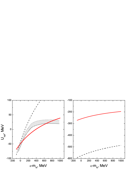
Figure 1: Energy dependence of the nucleon (left) and antinucleon (right) optical potentials. Solid lines – predictions of our model and dash lines, of the original Walecka model. Shaded area shows uncertainties in extrapolation from finite nuclei to cold nuclear matter [27].

There are mean-field solutions of the baryon and $\sigma,\omega,\rho$ meson Lagrangian $\sum_{b\in\{b\}}\mathcal{L}_{b}+\sum_{m\in\{m\}}\mathcal{L}_{m}^{\rm MF}$ [6]. To these terms we add the Lagrangian density for all meson excitations

$$\mathcal{L}_{\rm ex}=\sum_{ex\in\{ex\}}\mathcal{L}_{ex},\ \ \ \{ex\} = \pi^{\pm,0}(138);K^{\pm,0},\bar{K}^{0}(495);\eta(547);$$

$$K^{*\pm,0}(892),\eta^{\prime}(958),\phi(1020);\sigma^{\prime},\omega^{\prime},\rho^{\prime}.$$

The set $\{g\}=(\pi,K,\eta)$ is often treated as (quasi)Goldstone (index ”$g$”) bosons within the chiral SU(3) symmetrical models. Therefore, one may not scale their masses and couplings, as we have carried out for the mean fields $\sigma,\omega,\rho$, cf. the set $A$ for couplings in Fig. 8 (left) of ref. [6] . On the other hand, one may observe, cf. [6, 9], that for the case of spatially homogeneous system the equations for mean fields and thus their mean-field solutions do not change if one replaces the $\sigma$, $\omega_{0}$, $R_{0}$ fields by the scaled fields $\chi_{\sigma}\sigma$, $\chi_{\omega}\omega_{0}$ and $\chi_{\rho}R_{0}$, provided $\Phi_{b}=\Phi_{m}=\chi_{m}$, and $\chi_{\rho}^{\prime}=\chi_{\rho}^{2}$ ($\chi_{\rho}^{\prime}$ is the scaling function of the $\rho-\rho$ interaction $g_{\rho}$, see [6]). If one wishes to extend this symmetry to the case when Goldstones are included, in addition to the scaling of masses one should scale couplings, $g^{*}_{mg}=g_{mg}\ \chi_{m}$, cf. set $B$ in Fig. 8 (right) of [6]. In [6], we tested both possibilities $g^{*}_{mg}=g_{mg}$ and $g^{*}_{mg}=g_{mg}\ \chi_{m}$, and referred to them as versions without and with scaling, respectively. We include interaction of (quasi)Goldstones with mean fields (for $K$ and $\eta$, for $\pi$ it is small). As the result of this interaction, at sufficiently large (overcritical) baryon densities there may appear mean field solutions for (quasi)Goldstone fields signaling of condensations of these fields. Values of critical densities are higher for the set $B$. Since there are no experimental indications of condensation of (quasi)Goldstone bosons in the heavy ion collision regimes, comparing our results with experimental data, as in [6], we will focus on the set $B$, where condensates do not occur. $K^{*\pm,0},\eta^{\prime},\phi$ are assumed not to couple with mean fields, since there is no experimental information for such a coupling.

When the total Lagrangian is constructed, one can derive the equations of motion for every field. Even for low baryon density, the equations of motion for $\sigma$, $\omega$ and $\rho$ allow mean-field solutions $\sigma_{0}$, $\omega_{0}$, $\rho^{3}_{0}$. Therefore, we use

$$\sigma\equiv\sigma_{0};\quad\omega_{\mu}=\omega_{0}\ \delta_{\omega 0};\quad\rho_{\mu}^{a}=R_{0}\ \delta_{a3}\ \delta_{\mu 0}.$$ (7)

We assume that the system volume is sufficiently large and surface effects may be disregarded. Thus, only spatially homogeneous RMF solutions of the equations of motion are considered.

3 Improved description of meson excitations

The thermodynamic potential density $\Omega$, pressure $P$, free energy density $F$, energy density $E$ and entropy density $S$ are related as

$$E=F+TS,\quad F[f,\omega_{0},R_{0}]=\sum_{i}\mu_{i}n_{i}+\Omega\,,\quad\Omega=-P,$$ (8)

$$\mu_{i}=\frac{\partial F}{\partial n_{i}}\,.$$ (9)

Summation index $i$ runs over all particle species; $n_{i}$ are particle densities. Chemical potentials $\mu_{i}$ enter into the Green functions in the standard gauge combinations $\varepsilon_{i}+\mu_{i}$.

Thermodynamic quantities (8) can be found from the energy-momentum tensor $T_{\mu\nu}$ which is defined by our Lagrangian. The energy density $E$ and pressure $P$ are given by the diagonal terms of this tensor

$$E=\left<T_{00}\right>,\ \ \ \ \ \ P=\frac{1}{3}\left<T_{ii}\right>~{}.$$ (10)

In [6], the energy was chosen as a generating functional. Here we will use the pressure functional since it is more suitable to treat meson excitation effects in the presence of the mean fields and baryon-loop contributions.

3.1 Pressure at finite density and temperature

The pressure can be presented as the sum of the mean $\sigma$-, $\omega$-, $\rho$-field terms as well as of contributions of baryons and of all meson excitations. So we have

$$P[f,\omega_{0},R_{0}] = \sum_{m\in\{m\}}P^{\rm MF}_{m}[f,\omega_{0},R_{0}]+\sum_{b\in\{b\}}P_{b}[f,\omega_{0},R_{0}]$$ (11)

$$+ P_{\rm bos.ex.}[f,\omega_{0},R_{0}]~{}.$$

The first two sums are included in every RMF model but with a smaller set $\{b\}$, whereas the boson excitation term $P_{\rm bos.ex.}$ is constructed in [6] beyond the scope of the RMF approximation and will be further elaborated here.

Although in our treatment of the $\sigma$ variable all terms in (11) are functions only of $f$ and $T$, we also present them as functions of $\omega_{0}$ and $R_{0}$ in such a way that values of the $\omega_{0}(f)$ and $R_{0}(f)$ mean fields can be found by minimization of the pressure. Then $\omega_{0}(f)$ and $R_{0}(f)$ are plugged back in the pressure functional that becomes a function of $f$ only. The equilibrium value of $f$ can be found by subsequent minimization of the resulting pressure in this field.

In a self-consistent treatment, equations of motion for the mean fields render

$$\frac{\partial}{\partial\omega_{0}}\,P[f,\omega_{0}]=0\,~{},\quad\frac{\partial}{\partial R_{0}}\,P[f,R_{0}]=0\,,$$ (12)

and

$$\frac{d}{df}\,P[f,\omega_{0}(f),R_{0}(f)]=\frac{\partial}{\partial f}\,P[f,\omega_{0}(f),R_{0}(f)]=0\,$$ (13)

with pressure $P$ given by eq. (11). Since $P_{\rm bos.ex.}[f,\omega_{0},R_{0}]$ depends on the mean fields, its minimization produces extra terms in the equations of motion for the mean fields. In differentiating in (13) we used (12). This self-consistency of the scheme allows us to be sure of thermodynamic consistency of the model.

In [6], excitations were treated perturbatively. Accordingly, we assumed that $P_{\rm bos.ex.}=P_{\rm bos.ex.}[f^{\rm MF},\omega_{0}^{\rm MF},R_{0}^{\rm MF}]$, where $f^{\rm MF},\omega_{0}^{\rm MF},R_{0}^{\rm MF}$ are found by minimization of the pressure without inclusion of the boson excitation term. Thus, equations of motion for mean fields that we used in [6] are:

$$\frac{\partial}{\partial\omega_{0}}\,\left[\sum_{m\in\{m\}}P^{\rm MF}_{m}[f,\omega_{0},R_{0}]+\sum_{b\in\{b\}}P_{b}[f,\omega_{0},R_{0}]\right]=0\,~{},$$

$$\frac{\partial}{\partial R_{0}}\,\left[\sum_{m\in\{m\}}P^{\rm MF}_{m}[f,\omega_{0},R_{0}]+\sum_{b\in\{b\}}P_{b}[f,\omega_{0},R_{0}]\right]=0\,$$ (14)

and

$$\frac{d}{df}\,\left[\sum_{m\in\{m\}}P^{\rm MF}_{m}[f,\omega_{0},R_{0}]+\sum_{b\in\{b\}}P_{b}[f,\omega_{0},R_{0}]\right]$$

$$=\frac{\partial\,}{\partial f}\left[\sum_{m\in\{m\}}P^{\rm MF}_{m}[f,\omega_{0},R_{0}]+\sum_{b\in\{b\}}P_{b}[f,\omega_{0},R_{0}]\right]=0\,.$$ (15)

Equation (14) was used in differentiating in (15). Below in Figs. 2–5 we demonstrate how effects of a nonperturbative treatment of boson excitations, incorporated in (12) and (13) (a self-consistent analysis) and neglected in (14), (15), affect results of the SHMC model.

Actually, in [6] instead of varying the pressure at fixed chemical potentials $\mu_{i}$ and the temperature $T$, we varied the energy density under the condition that one should not vary it with respect to the particle occupation numbers. When $E$ is varied, one should fix the particle densities $n_{i}$ and the entropy densities $S_{i}$, which is equivalent to fixed particle occupations in our quasiparticle approach. Two procedures mentioned are equivalent, provided baryon-baryon hole and baryon-antibaryon excitation effects (loop contributions) are disregarded (as we did in (12) – (15)). An attempt to incorporate the baryon loop corrections into our scheme has been done in Appendix B.

Now let us consider partial contributions to the pressure in eq. (11).

3.2 The baryon contribution

The contribution of the given baryon (antibaryon) species $b\in\{b\}$ to the pressure is as follows:

$$P_{b}[f,\omega_{0},R_{0}] = \frac{1}{3}(2s_{b}+1)\intop_{0}^{\infty}\frac{{\rm d}p\ p^{4}}{2\pi^{2}}\,\frac{f_{b}}{\omega_{b}}-t^{Q}_{b}\ n_{b}\ \mu_{\rm ch}~{},$$ (16)

$$p=|\vec{p}|,\quad\omega_{b}=\sqrt{m_{b}^{*2}(f)+p^{2}}.$$

The spin factor $s_{b}=1/2$ for nucleons ($N$) and hyperons, while $s_{b}=3/2$ for $\Delta$-resonances.

The baryon set $\{b\}$ to be used (taken from Table 1 of [6]) was fixed above, see after eq. (1). Little differences in masses of charged and neutral particles of the given species are ignored. Also we ignore small inhomogeneous Coulomb field effects and put the electric potential $V=0$. The charge chemical potential $\mu_{\rm ch}$ is then related to the isospin composition of the system. For the isospin-symmetric system, $N=Z$, one has $\mu_{\rm ch}=0$.

The Fermi-particle (baryon/antibaryon) occupation

$$f_{b} = \frac{1}{\exp[(\omega_{b}-\mu_{b}^{*})/T]+1}\quad$$ (17)

depends on the gauge-shifted values of the chemical potentials

$$\mu_{b}^{*}=t_{b}\ \mu_{{\rm bar}}+t^{s}_{b}\ \mu_{{\rm str}}+t^{Q}_{b}\mu_{\rm ch}-g_{\omega b}\ \chi_{\omega}\omega_{0}-t^{3}_{b}\ g_{\rho b}\ \chi_{\rho}\ R_{0}~{}.$$ (18)

The baryon/antibaryon chemical potential of the $b$-species is $\mu_{b}=t_{b}\ \mu_{{\rm bar}}$, and the corresponding strangeness term is $\mu^{s}_{b}=t^{s}_{b}\ \mu_{{\rm str}}$. Baryon quantum numbers $t_{b}$, $t_{s}^{b}$, $t_{b}^{3}$ and $t_{b}^{Q}$ are baryon charge, strangeness, isospin projection and electric charge, respectively, and proper charge conjugated values for antiparticles are given in Table 1 in [6].

3.3 Mean-field contribution

It is convenient to introduce the coupling ratios

$$x_{mb}=g_{mb}/g_{mN},\,\,\,m\in\{m\}=\sigma,\omega,\rho,$$ (19)

and, instead of $\chi_{m}$, other variables

$$\eta_{m}(f)={\Phi_{m}^{2}(f)}/{{\chi}_{m}^{2}(f)}\,,$$ (20)

since the pressure depends namely on this sort of combinations rather than on $\Phi_{m}$ and $\chi_{m}$ separately.

In terms of these new variables the contribution of mean fields to the pressure is as follows:

$$P^{\rm MF}_{\sigma}[f]=-\frac{m_{N}^{4}\,f^{2}}{2\,C_{\sigma}^{2}}\,\eta_{\sigma}(f)-{U}(f),$$ (21)

$$P^{\rm MF}_{\omega}[f,\omega_{0}]=\frac{m_{N}^{2}\eta_{\omega}(f)}{2\,C_{\omega}^{2}}\left[g_{\omega N}\,{\chi}_{\omega}\,\omega_{0}\right]^{2}\,,$$ (22)

$$P^{\rm MF}_{\rho}[f,R_{0}]=\frac{m_{N}^{2}\ \eta_{\rho}(f)}{2\,C_{\rho}^{2}}\left[g_{\rho N}\,{\chi}_{\rho}\ R_{0}\right]^{2}\!.$$ (23)

Here the renormalized constants are

$$C_{m}=\frac{m_{N}\ g_{mN}}{m_{m}}.$$ (24)

The net baryon density is given by [6]:

$$n_{B}\equiv\sum_{b\in\{b\}}t_{b}n_{b}~{},\quad n_{b}=(2s_{b}+1)\intop_{0}^{\infty}\frac{{\rm d}p\ p^{2}}{2\pi^{2}}\,f_{b}~{},$$ (25)

where $n_{b}$ is the baryon (antibaryon) number density and occupation baryon (antibaryon) density is defined by eq. (17). On the other hand, for fixed baryon species the contribution to the baryon density should obey the thermodynamic consistency condition

$$n_{b}=\left.\frac{\partial P}{\partial\mu_{b}^{*}}\right|_{T}.$$ (26)

Both quantities presented by (26) and (25) coincide provided contributions of boson excitations do not depend on the baryon loop terms (see Appendix B). In this case thermodynamic consistency of the model is preserved, see below in more detail.

The isotopic charge density in the baryon sector is given by

$$n^{t}_{B}=2\sum_{b\in\{b\}}\ t_{b}^{3}\ n_{b}\ x_{\rho b}~{}.$$ (27)

The isovector baryon density $n^{t}_{B}$ plays the role of the source for the $\rho$-meson field $\rho_{0}^{(3)}=R_{0}$ . Therefore, for the iso-symmetrical matter ($N=Z$) one has $n^{t}_{B}=0$ and $P^{\rm MF}_{\rho}=0$ .

The net strangeness density of baryons and mesons reads

$$n_{\rm str}=\sum_{i\in\{b\},\{\rm ex\}}t_{i}^{s}\ n_{i}~{}.$$ (28)

Bearing in mind applications of the model to high-energy heavy ion collisions from AGS to RHIC energies we assume that all strange particles are trapped inside the fireball till the freeze-out. Therefore, the total strangeness is zero. Thus, we put $n_{\rm str}=0$. This condition determines the value of the strangeness chemical potential $\mu_{\rm str}$.

Similarly, we may introduce the electric charge density

$$n_{\rm ch}=\sum_{i\in\{b\},\{ex\}}t_{i}^{Q}\ n_{i}~{}.$$ (29)

The quantity $n_{\rm ch}=(Z/A)n_{B}$ determines the value of the charged chemical potential $\mu_{\rm ch}$. For the symmetric matter, $N=Z$, ignoring Coulomb effects one may put $\mu_{n}=\mu_{p}$ and $\mu_{\rm ch}=0$.

Our SHMC model pressure functional depends on four particular combinations of functions, $\eta_{\sigma,\rho,\omega}(f)$ and $U(f)$. Note that the dependence on the scaling function $\eta_{\sigma}$ can always be presented as part of the new potential $U$ obtained by means of the replacement $U\to U+\frac{m_{N}^{4}\,f^{2}}{2\,C_{\sigma}^{2}}\,(1-\eta_{\sigma}(f))$ , and vice versa, so the potential $U$ can be absorbed in the new quantity $\eta_{\sigma}$. Thus actually only three independent functions enter into the pressure functional. Equation (11) together with eqs. (16), (21), (22), (23) demonstrates explicitly the equivalence of mean-field Lagrangians for constant fields with various parameters if they correspond to the same functions $\eta_{\rho,\omega}(f)$ and $\eta_{\sigma}$ (either $U(f)$) with the field $f$ related to the scalar field $\sigma$ through eq. (3). In [6], we assumed $\eta_{\sigma}=1$. Here we accept the same choice.

3.4 Bosonic excitations

To find the total pressure (11), one should define the contribution of bosonic excitations. Within our model and in agreement with [6] it is the sum of partial contributions

$$P_{\rm bos.ex}[f,\omega_{0},R_{0},T] = P_{\sigma}^{\rm part}+P_{\omega}^{\rm part}+P_{\rho}^{\rm part}+P_{\pi}^{\rm part}$$ (30)

$$+ P_{K}^{\rm part}+P_{\eta}^{\rm part}+P_{K^{*}}^{\rm part}+P_{\eta^{\prime}}^{\rm part}+P_{\phi}^{\rm part}~{}.$$

The pressure of the pion gas is

$$P_{\pi}^{\rm part} = P_{\pi^{+}}+P_{\pi^{0}}+P_{\pi^{-}}=\frac{1}{3}\intop_{0}^{\infty}\frac{{\rm d}p\ p^{4}}{2\pi^{2}}\,$$

$$\times \left[\frac{f_{\pi^{+}}(\omega_{\pi^{+}}(p))}{\omega_{\pi^{+}}(p)}+\frac{f_{\pi^{0}}(\omega_{\pi^{0}}(p))}{\omega_{\pi^{0}}(p)}+\frac{f_{\pi^{-}}(\omega_{\pi^{-}}(p))}{\omega_{\pi^{-}}(p)}\right]~{}.$$

Due to the absence of the $\omega\rightarrow 2\pi$ decay the coupling $g_{\omega\pi}^{*}=0$. For $N=Z$, the field $R_{0}=0$ and dependence of pion spectra on $g_{\rho\pi}^{*}$ disappears. Also, as in [6], we suppose $g_{\sigma\pi}^{*}=0$ ignoring a small pion mass shift. Then for both charged and neutral pions we may use

$$\omega_{\pi^{\pm}}(p)=\omega_{\pi^{0}}(p)=\sqrt{m_{\pi}^{2}\,+p^{2}}.$$ (32)

The pressure of the kaon gas is given as follows

$$P_{{K}}^{\rm part} = P_{K^{+}}+P_{K^{0}}+P_{K^{-}}+P_{\bar{K}^{0}}$$

$$= \frac{1}{3}\intop_{0}^{\infty}\frac{{\rm d}p\ p^{4}}{2\pi^{2}}\,\left[\frac{f_{K^{+}}(\omega_{K^{+}}(p))}{\omega_{K^{+}}(p)}+\frac{f_{K^{0}}(\omega_{K^{0}}(p))}{\omega_{K^{0}}(p)}\right]$$

$$+ \frac{1}{3}\intop_{0}^{\infty}\frac{{\rm d}pp^{4}}{2\pi^{2}}\,\left[\frac{f_{K^{-}}(\omega_{K^{-}}(p))}{\omega_{K^{-}}(p)}+\frac{f_{\bar{K}^{0}}(\omega_{\bar{K}^{0}}(p))}{\omega_{\bar{K}^{0}}(p)}\right]~{},$$

where

$$\omega_{K^{\pm}}(p)=\pm g_{\omega K}^{*}\ \omega_{0}\pm g_{\rho K}^{*}\ R_{0}+\sqrt{m_{K}^{*2}\,+p^{2}}~{},\quad m_{K}^{*}=m_{K}-g_{\sigma K}^{*}\sigma$$ (34)

and $g_{mK}^{*}=g_{mK}\chi_{m}$ for the parameters of the set $B$ [6], we use here. Note that in neglecting Coulomb effects the energy of $K^{+}$ coincides with that for $K^{0}$ and the energy of $K^{-}$ coincides with the $\bar{K}^{0}$ energy.

The $\eta$-contribution to the pressure is given by

$$P_{\eta}^{\rm part} = \frac{1}{3}\intop_{0}^{\infty}\frac{{\rm d}p\ p^{4}}{2\pi^{2}}\,\frac{f_{\eta}(\omega_{\eta}(p))}{\omega_{\eta}(p)}~{},\quad\omega_{\eta}=\sqrt{m_{\eta}^{*2}+{p}^{2}}$$ (35)

with

$$m_{\eta}^{*2}=\left(m_{\eta}^{2}-\sum_{b\in\{b\}}\frac{\Sigma_{\eta b}}{f^{2}_{\pi}}\left<\bar{\Psi}_{b}\,\Psi_{b}\right>\right)/\left(1+\sum_{b\in\{b\}}\frac{\kappa_{\eta b}}{f^{2}_{\pi}}\left<\bar{\Psi}_{b}\,\Psi_{b}\right>\right)$$ (36)

expressed in ref. [29] in terms of the total baryon scalar density $\sum_{b\in\{b\}}\ n_{sb}=\\ \sum_{b\in\{b\}}\left<\bar{\Psi}_{b}\,\Psi_{b}\right>$.

In the above equations the Bose distributions of excitations are

$$f_{\rm i} = \frac{1}{\mbox{exp}[(\sqrt{m_{\rm i}^{*2}+p^{2}}-\mu_{\rm i}^{*})/T]-1},$$ (37)

$$\mu_{\rm i}^{*} = \mu_{\rm i}+Q_{\rm i}\mu_{\rm ch}-Q^{\rm vec}_{\rm i}\ g_{\omega{\rm i}}^{*}\ \omega_{0}-Q^{\rm vec}_{\rm i}g_{\rho{\rm i}}^{*}R_{0},$$

$$i\in\{{\rm bos.ex}\} = \sigma^{{}^{\prime}},\omega^{{}^{\prime}},\rho^{{}^{\prime}+},\rho^{{}^{\prime}0},\rho^{{}^{\prime}-};\pi^{+},\pi^{0},\pi^{-};K^{+},K^{0},K^{-},\bar{K}^{0};\eta;$$

$$K^{*+},K^{*0},K^{*-},\bar{K}^{*0};\eta^{{}^{\prime}};\varphi~{}.$$

Here $\mu_{i}=\mu_{\rm str}$ for strange particles $K$ and $K^{*}$ and $\mu_{i}=-\mu_{\rm str}$ for their anti-particles; $Q_{\rm i}$ is the boson electric charge in proton charge units (ignoring Coulomb effects we put $Q_{i}=0$), $Q^{\rm vec}_{\rm i}=+1$ for particle, $Q^{\rm vec}_{\rm i}=-1$ for antiparticle and $Q^{\rm vec}_{\rm i}=0$ for ”neutral” particles (with all zero charges including strangeness). We take couplings as in [6], $g_{mi}^{*}=0$ for all $i$ except $i=K,\eta$. For $\eta$ we select the parameter choice $\Sigma_{\eta b}=140$ MeV, $\kappa_{\eta b}=0.2$. As in [6] we assume $m^{*}_{K^{*}}=m_{K^{*}}$, $m^{*}_{\eta^{{}^{\prime}}}=m_{\eta^{{}^{\prime}}}$, $m^{*}_{\varphi}=m_{\varphi}$ due to the absence of the corresponding experimental data. In this paper, we will focus on the consideration of the isospin-symmetrical matter; therefore, we may put $R_{0}=0$.

The density of the gas of Bose excitations of the given species $i$ is determined by the integral

$$n_{i}=g_{i}\intop_{0}^{\infty}\frac{{\rm d}p\ p^{2}}{2\pi^{2}}\,f_{i}(p)~{},\quad i\in\{{\rm bos.ex}\},$$ (38)

where $g_{i}$ is the corresponding degeneracy factor.

Note that the $p$-wave pion and kaon terms can easily be included. For that one needs to replace $\omega_{\pi}(p)$ and $\omega_{K}(p)$ with more complicated expressions, see refs. [24, 26]. In order to obtain the temperature-density dependent pion and kaon spectral functions one needs to calculate the pion and the kaon self-energies including baryon-baryon hole loops and baryon-baryon correlation effects. These effects may result in appearance of the pion and antikaon condensates in dense and not too hot nuclear matter. Within the SHMC model we incorporate only interactions of particles through mean fields. Even in this case many coupling constants are not well fixed due to the lack of experimental data. Thus, we postpone the inclusion of the $p$-wave interactions to the future work.

A more nontrivial task is to fix the terms $P_{\sigma}^{\rm part}$, $P_{\omega}^{\rm part}$, $P_{\rho}^{\rm part}$. For the $\sigma^{{}^{\prime}}$, $\omega^{{}^{\prime}}$, $\rho^{{}^{\prime}}$ contributions to the pressure we use the standard ideal gas expressions with effective masses determined as follows. Let us first focus on the contribution of the $\sigma^{{}^{\prime}}$-excitations. In order to get $P_{\sigma}^{\rm part}$, we should expand total pressure $P[\sigma,\omega_{0}(\sigma),R_{0}(\sigma)]$ in $\sigma^{{}^{\prime}}=\sigma-\sigma^{\rm cl}$. The term linear in $\sigma^{{}^{\prime}}$ does not give a contribution due to subsequent requirement of the pressure minimum in $\sigma^{\rm cl}$. The quadratic term produces effective $\sigma$ particle mass squared,

$$(m_{\sigma}^{\rm part*})^{2}=-\frac{{d^{2}P[\sigma,\omega_{0}(\sigma),R_{0}(\sigma)]}}{{d\sigma^{2}}}=-\frac{{d^{2}P[f,\omega_{0}(f),R_{0}(f)]}}{{df^{2}}}\left(\frac{df}{d\sigma}\right)^{2}.$$ (39)

The first-order derivative $dP/df=0$, as it follows from the equations of motion. Since we deal with the strong interaction problem and the general solution is impossible, one should use some approximations. First, keeping only quadratic terms in all thermodynamical quantities in boson fluctuating fields we disregard boson excitation contributions to the $\sigma^{{}^{\prime}}$, $\omega^{{}^{\prime}}$, $\rho^{{}^{\prime}}$ effective masses (higher order effects in boson fluctuating fields). Within this approximation we neglect the $P_{\rm bos.ex.}$ term in (39). Moreover, our aim is the construction of a thermodynamically consistent model where the baryon density and the entropy density, calculated by using the thermodynamic relation (26) and relation

$$S=\left.\frac{\partial P}{\partial T}\right|_{\mu}~{},$$ (40)

coincide with quasiparticle expressions (25) and

$$S=S_{\rm bar}+S_{\rm bos.ex.},\quad S_{\rm bar}=\sum_{b\in\{b\}}g_{b}\int\frac{{\rm d}p_{b}\ p_{b}^{2}}{2\pi^{2}}[-(1-f_{b})\mbox{ln}(1-f_{b})-f_{b}\mbox{ln}f_{b}],$$

$$S_{\rm bos.ex.}=\sum_{i\in\{\rm bos.ex.\}}g_{i}\int\frac{{\rm d}p_{i}\ p_{i}^{2}}{2\pi^{2}}[(1+f_{i})\mbox{ln}(1+f_{i})-f_{i}\mbox{ln}f_{i}],$$ (41)

namely, the latter expressions in ref. [6]. In order to keep thermodynamic consistency of the model, we suppress the baryon contribution in (39). This term is associated with taking into account of the baryon-antibaryon and baryon-baryon hole loops. Problems arisen, if one includes baryon loops, are discussed in Appendix B.

Thus, the squared effective mass of the $\sigma^{{}^{\prime}}$ excitation will be given by the expression

$$(m_{\sigma}^{\rm part*})^{2}\simeq-\sum_{m\in\{m\}}\frac{{d^{2}P_{m}^{\rm MF}[f,\omega_{0}(f),R_{0}(f)]}}{{df^{2}}}\left(\frac{df}{d\sigma}\right)^{2}.$$ (42)

Using the relation $\chi_{\sigma}=\Phi=1-f$ we find that

$$\frac{df}{d\sigma}=\frac{g_{\sigma N}}{m_{N}}(1-f)^{2}.$$ (43)

For the isospin-symmetrical nuclear matter $N=Z$, we obtain

$$(m_{\sigma}^{\rm part*})^{2}=\left[U^{{}^{\prime\prime}}_{f}+\frac{m_{N}^{4}}{C_{\sigma}^{2}}\right]\left(\frac{g_{\sigma N}}{m_{N}}\right)^{2}(1-f)^{4}.$$ (44)

One could use a different approximation introducing the effective mass term with the help of the expression for the Hamiltonian (Lagrangian). In the latter case, baryon terms are added to the meson mean field contribution and derivatives of the Hamiltonian are taken at fixed $\Psi_{B}$. In this case

$$(m_{\sigma}^{\rm part*})^{2}=\left<\frac{{d^{2}H}}{{d\sigma^{2}}}\right>=\left<\frac{{d^{2}H}}{{df^{2}}}\right>\left(\frac{df}{d\sigma}\right)^{2},$$ (45)

where $H$ is the Hamiltonian and the averaging procedure is carried out over a thermal equilibrium state after taking the derivatives. We used that $\left<\frac{{dH}}{{d\sigma}}\right>=0$, as it follows from the equations of motion. Neglecting the meson excitation terms in $H$ we find

$$\left<\frac{{d^{2}H}}{{df^{2}}}\right> = -\sum_{m\in\{m\}}\frac{{d^{2}P_{m}^{\rm MF}[f,\omega_{0}(f),T]}}{{df^{2}}}+\left<\sum_{b\in\{b\}}\frac{{d^{2}H_{b}[f,\omega_{0}(f),T]}}{{df^{2}}}\right>$$ (46)

$$= U^{{}^{\prime\prime}}_{f}+\frac{m_{N}^{4}}{C_{\sigma}^{2}}+\frac{C_{\omega}^{2}}{2m_{N}^{2}}\left(\frac{d^{2}}{df^{2}}\frac{1}{\eta_{\omega}}\right)\sum_{b}x_{\omega b}\ n_{sb},$$

where the baryon (antibaryon) scalar density $n_{sb}$ is given by

$$n_{sb}=(2s_{b}+1)\int_{0}^{\infty}\frac{dpp^{2}}{2\pi^{2}}\frac{m_{b}^{*}}{\omega_{b}}f_{b}.$$

Since in ref. [6] the value $\eta_{\omega}^{-1}$ was chosen as a linear function of $f$,

$$\eta_{\omega}^{-1}=(1+zf)/(1+zf(n_{0})),\quad z=const,$$ (47)

($z=0.65$ in the KVOR-based SHMC model), we get $\sum_{b\in\{b\}}\frac{{d^{2}H_{b}[f,\omega_{0}(f),T]}}{{df^{2}}}=0$, and both results (42) and (45) coincide. From here it is seen that in our approximation $(m_{\sigma}^{\rm part*})^{2}$ does not explicitly depend on the baryon variables and the temperature. Obviously, within this approximation our model remains thermodynamically consistent since meson excitation terms in the pressure do not contribute to the derivatives of the pressure over the baryon chemical potential (to obtain $n_{B}$) and over the temperature (to get entropy $S$).

Note that in [6] we introduced the squared effective mass of the $\sigma^{{}^{\prime}}$-excitation as the second derivative of the energy density. Since at the same time the contributions of all baryon particle-particle hole and particle-antiparticle (loop) terms were suppressed, this result coincides with expressions (42) and (45).

Within our approximation the masses of vector particles are given by

$$(m_{\omega_{i}}^{\rm part*})^{2}=\left<\frac{{\partial^{2}H}}{{\partial\omega_{i}^{2}}}\right>=-\sum_{m\in\{m\}}\frac{{\partial^{2}P_{m}^{\rm MF}[f,\omega_{0}]}}{{\partial\omega_{i}^{2}}},$$ (48)

$$(m_{\rho_{i}}^{\rm part*})^{2}=\left<\frac{{\partial^{2}H}}{{\partial R_{i}^{2}}}\right>=-\sum_{m\in\{m\}}\frac{{\partial^{2}P_{m}^{\rm MF}[f,\omega_{0}]}}{{\partial R_{i}^{2}}},\quad i=0,1,2,3.$$

In this case zero-components of one $\omega$ and three $\rho$-excitations prove to be the same as those following from the mean-field mass terms

$$m_{\omega}^{\rm part*}=m_{\omega}|\Phi_{\omega}(f)|,\quad m_{\rho}^{\rm part*}=m_{\rho}|\Phi_{\omega}(f)|~{}.$$ (49)

Moreover, there are excitations of two magnetic-like components of $\omega$ and six magnetic-like components of $\rho$. Their masses are given by eqs. (49) since there are no $\vec{\omega}$ and $\vec{R}$ mean fields, namely, expressions (49) were used in [6].

Thus, neglecting the baryon and boson excitation contributions to the effective meson excitation masses we obtain a rather simple thermodynamically consistent description.

3.5 Some numerical results

In Figs. 2, 3 we demonstrate the size of corrections which arise provided boson excitations are incorporated in the equations of motion. Particle excitation masses are calculated following eq. (42) for $\sigma$ meson excitation and (49) for the nucleon, $\omega$, and $\rho$ excitations. Figure 2 demonstrates the ratio of the effective masses to the bare masses for the nucleon-$\omega^{{}^{\prime}}$-$\rho^{{}^{\prime}}$ (left panel) and for $\sigma^{{}^{\prime}}$ (right panel) as a function of the temperature at $n_{B}=0$ (thin curves) and at $n_{B}=5~{}n_{0}$ (bold lines). Solid curves are calculations of the given paper, when boson excitations contribute to the equations of motion, whereas dashed curves show perturbative calculations of ref. [6]. Although for $T\stackrel{{\scriptstyle\scriptstyle>}}{{\phantom{}{}_{\sim}}}120$ MeV there appear pronounced differences between both treatments of excitations, the qualitative behavior remains unchanged. Effective masses of all excitations exhibit a similar behavior as functions of the temperature and the density, in a line with the mass-scaling hypothesis that we have exploited for the mean fields.

Let us also compare our result for $N$, $\omega$, $\rho$ effective masses (Fig. 2 left) with that previously obtained in the model of ref. [13], their Fig. 1 left (for $N$) and right (for $\omega,\rho$). Shapes of the curves look similar. However in our case $N$, $\omega$, $\rho$ are scaled by one scaling function, whereas ref. [13] used different scalings for $N$ and for $\omega,\rho$. In their case the masses drop much stronger with the density increase but remain finite at high temperatures ($T\stackrel{{\scriptstyle\scriptstyle>}}{{\phantom{}{}_{\sim}}}200$ MeV), whereas in our case they drop to zero at $T_{c}\sim 210$ MeV.

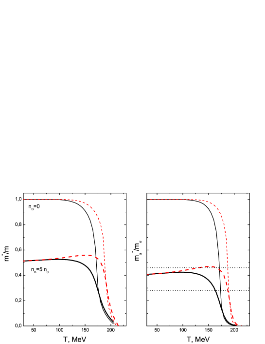
Figure 2: Temperature dependence of the effective-to-bare mass ratio for nucleon-$\omega^{{}^{\prime}}$-$\rho^{{}^{\prime}}$ (left panel) and for $\sigma^{{}^{\prime}}$ (right panel) for $n_{B}=0$ and $n_{B}=5~{}n_{0}$. The solid lines are our results, the dashed ones are perturbative calculations from [6]. To guide the eye, the horizontal dots show the $m_{\sigma}^{*}=2m_{\pi}$ and $m_{\sigma}^{*}=m_{\pi}$ thresholds.

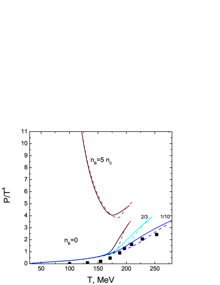
Figure 3: Temperature dependence of the reduced pressure. Solid lines show calculations of the given work, whereas dashed lines demonstrate the results of the perturbative treatment of boson excitations [6]. The curves labeled by $2/3$ and $1/10$ correspond to the case when all $g_{\sigma b}$ couplings except for nucleons are suppressed by factors $2/3$ and $1/10$, respectively. Filled squares show the lattice QCD result for the 2+1 flavor case [30].

The effect of the mentioned nonperturbative treatment of boson excitations on thermodynamic quantities is presented in Fig. 3. The temperature dependence is shown for the reduced pressure calculated in the given work (solid lines) and in the perturbative treatment of boson excitations [6] at $n_{B}=0$ and $n_{B}=5n_{0}$. One can see that the differences are rather noticeable only in the temperature interval $170<T<200$ MeV, provided the baryon-meson couplings are not artificially suppressed. In the case ($n_{B}=0$), when all $g_{\sigma b}$ couplings except for nucleons are artificially suppressed by factors $2/3$ and $1/10$, the temperature interval, where solid and dash curves deviate from each other, is broader but the value of the deviation is smaller. The curve for $g_{\sigma b}$ suppressed by $1/10$ reasonably matches the lattice data for $T_{c}<T\stackrel{{\scriptstyle\scriptstyle<}}{{\phantom{}{}_{\sim}}}230$ MeV. As has been mentioned in [6] one could fit the lattice data even in a broader region of temperatures (up to $500~{}$MeV) if one introduced $\chi_{\sigma}<\Phi$. A violation of the universality of the $\sigma$ scaling would be also in a line with that we have used for $\omega$ and $\rho$, $\eta_{\omega}\neq 1$ and $\eta_{\rho}\neq 1$, as required to describe properties of neutron stars, cf. [26]. However we will not elaborate such a possibility in the present work. Instead we simply suppress $g_{\sigma b},b\neq N$. Hydrodynamic simulations of heavy ion collisions are fully determined by the EoS to be described with quark and gluon degrees of freedom or with only hadron ones. With such an EoS (with suppressed $g_{\sigma b}$) a quark liquid would masquerade as a hadron one.

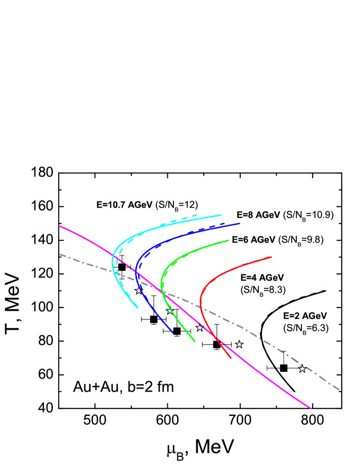
Figure 4: Isentropic trajectories for central Au+Au collisions at different bombarding energies calculated in the present paper (solid lines) and with the perturbative treatment of boson excitations [6] (dashed lines). The results are presented for the SIS-to-AGS energies. Experimental points with error bars are taken from [31]. The freeze-out points marked by stars are obtained in [6]. Thin line corresponds to the freeze-out curve in [31] while dash-dotted line is that from [32].

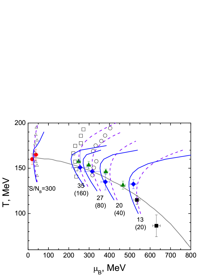
Figure 5: Isentropic trajectories for central Au+Au collisions at different bombarding energies calculated in the present paper. Calculations are performed from AGS to RHIC energies for not suppressed couplings (solid lines) and with suppressed $g_{\sigma b}$ couplings (except for nucleons) by a factor of $1/10$ (dashed lines). The filled diamonds and triangles are obtained from the $4\pi$ particle ratios in [31] and [33], respectively. Filled circles are RHIC data based on the middle rapidity particle ratios [31]. Open circles, squares and triangles are the lattice 2-flavor QCD results [34] for $S/N_{B}=$ 30, 45 and 300, respectively. The thin line corresponds to the freeze-out curve in [31].

In Fig. 4 we show the isentropic trajectories for central Au+Au collisions at different bombarding energies calculated in the present paper (solid lines) and with the perturbative treatment of boson excitations from ref. [6] (dashed lines). As we can see from Fig. 4, for AGS energies the trajectories calculated here almost coincide with those computed in ref. [6] where boson excitations were treated perturbatively. Then, as in [6] we extend our analysis to higher bombarding energies. The entropy per baryon participants was calculated in [35] within the 3-fluid hydrodynamic model assuming occurrence of the first order phase transition to a quark-gluon plasma. The energy range from AGS to SPS was covered there. We use the $S/N_{B}$ values for $E_{lab}=$158, 80, 40 and 20 AGeV, at which the particle ratios were measured by the NA49 collaboration (cf. [31]). At the RHIC we put $S/N_{B}=300$ in accordance with an estimate in [34].

Since there is a reasonable fit of the lattice data on the pressure for $T\stackrel{{\scriptstyle\scriptstyle>}}{{\phantom{}{}_{\sim}}}200$ MeV with reduced meson-baryon coupling constants, see [6] and Fig. 3, for high collision energies we show in Fig. 5 both the results, when couplings are not suppressed (solid curves) and also when all $g_{\sigma b}$ couplings except for nucleons are suppressed by a factor of $1/10$. As is seen, the decrease in $g_{\sigma b}$ improves the high-temperature description (as compared to the case of not suppressed couplings) for the lattice data at high temperatures not only for the case $\mu_{b}=0$ but also for $\mu_{b}\neq 0$. For low temperatures the solid and dashed curves (the curves for not suppressed and suppressed $g_{\sigma b}$ couplings, respectively) are very close to each other. Also note that one should be rather critical performing comparison with the existing lattice data, especially for the case $\mu_{b}\neq 0$ (presented in Fig. 5 for 2 flavors). Doing this comparison we tentatively hope that results of future more realistic lattice calculations will not deviate much from the existing ones.

In all cases our new calculations presented in Fig. 5 (if one additionally suppresses couplings), as well as corresponding perturbative calculations [6], describe reasonably the lattice data on the $T-\mu_{B}$ trajectories and freeze out points.

Concluding, our improvement of the model with keeping boson excitation terms in the equations of motion neither spoils nor improves the agreement with the lattice results and with the thermodynamic parameters extracted at freeze out. Thus, both perturbative and nonperturbative treatments of boson excitation effects can be used with equal success. However, one should note that thermodynamic consistency conditions are fulfilled exactly in the non-perturbative treatment of the given work, whereas in the perturbative treatment of [6] they were satisfied only approximately.

4 Inclusion of finite resonance widths

In the framework of our model we treated all resonances as quasiparticles neglecting their widths. Excitations interact only with the mean fields. Thus imaginary parts of the self-energies as well as some contributions to the real parts are not taken into account. Definitely it is only a rough approximation carried out just for simplification.

At the resonance peak the vacuum $\Delta$-isobar mass width is $\Gamma_{\Delta}^{\rm max}\simeq 115$ MeV. In reality $\Gamma_{\Delta}$ is the temperature-, density- and energy-momentum-dependent quantity. For low $\Delta$-energies the width is much less than $\Gamma_{\Delta}^{\rm max}$. A typical $\Delta$ energy is $\omega_{\Delta}-m_{\Delta}^{*}\sim T$. Thus for low temperature, $T\stackrel{{\scriptstyle\scriptstyle<}}{{\phantom{}{}_{\sim}}}\epsilon_{F}$ ($\epsilon_{F}$ is the nucleon Fermi energy) the effective value of the $\Delta$-width is significantly less than $\Gamma_{\Delta}^{\rm max}$. At these temperatures the quasiparticle approximation does not work for $\Delta$’s but their contribution to thermodynamic quantities is small. When the temperature is $\stackrel{{\scriptstyle\scriptstyle>}}{{\phantom{}{}_{\sim}}}m_{\pi}$ there appears essential temperature contribution to the width and the resonance becomes broader [36]. At such temperatures $\Delta$’s essentially contribute to thermodynamic quantities. Only for temperatures $T\stackrel{{\scriptstyle\scriptstyle>}}{{\phantom{}{}_{\sim}}}\Gamma_{\Delta}^{\rm max}(T)$ the quasiparticle approximation becomes a reasonable approximation.

The $\rho$- and $\sigma$-mesons also have rather broad widths. E.g., at a maximum the $\rho$-meson width is about $150$ MeV. The observed enhancement of the dilepton production at CERN, in particular in the recent NA60 experiment [37] on $\mu^{+}\mu^{-}$ production, can be explained by significant broadening of the $\rho$ in matter [2], though decreasing of the $\rho$ mass could also help in explanation of the data [38]. Besides, as was shown in [40] to be consistent with the QCD sum rules, both the collisional broadening and dropping of the $\rho$ mass should be taken into account. Even more, one should be careful with interpretation of the NA60 experiment: Dileptons carry direct information on the $\rho$ meson spectral function only if the vector dominance is valid but generally it is not the case [41].

Also particles which have no widths in vacuum like nucleons acquire the widths in matter due to collisional broadening. Their widths grow with the temperature increase, cf. [42]. As we have argued above in case with $\Delta$ isobars, the quasiparticle approximation may become a reasonable approximation at sufficiently high temperature, if $T\stackrel{{\scriptstyle\scriptstyle>}}{{\phantom{}{}_{\sim}}}\Gamma(T)$.

Let us roughly estimate the effect of finite baryon and meson resonance widths on particle distributions and the EoS in order to understand how much and in which temperature-density regions these effects may affect results calculated within our quasiparticle SHMC model.

It is convenient to introduce single-particle spectral $\widehat{A}_{\rm r}$ and width $\widehat{\Gamma}_{\rm r}$ functions (operators), cf. [42],

$$\widehat{A}_{\rm r}=-2{\rm Im}\widehat{G}^{R}_{\rm r}(q)=-2{\rm Im}\frac{1}{\widehat{M}_{\rm r}+i\widehat{\Gamma}_{\rm r}/2},\,\,\,\ \ \widehat{\Gamma}_{\rm r}=-2{\rm Im}\widehat{\Sigma}^{R}_{\rm r}\,,$$ (50)

where $\widehat{G}_{\rm r}^{R}(q)$ is the full retarded Green function of the fermion and $\widehat{\Sigma}^{R}_{\rm r}$ is the retarded self-energy. The quantity

$$\widehat{M}_{\rm r}=(\widehat{G}^{0,R})^{-1}-{\rm Re}\widehat{\Sigma}^{R}_{\rm r}$$ (51)

demonstrates the deviation from the mass shell: $\widehat{M}_{\rm r}=0$ on the quasiparticle mass shell in the matter, $\widehat{G}^{0,R}$ is the free Green function. Following definition (50) the spectral function of the fermion has dimensionality of $m^{-1}$ and the width, dimensionality $m$, whereas for bosons the spectral function has dimensionality of $m^{-2}$ and the width, dimensionality $m^{2}$.

Let us start with the consideration of a fermion spin $1/2$ resonance (superscript $\rm f$). The spectral function satisfies the sum rule:

$$\frac{1}{4}\mbox{Tr}\int^{\infty}_{0}\gamma_{0}\left[\widehat{A}^{\rm f}_{\rm r(+)}(q_{0},\vec{q})+\widehat{A}^{\rm f}_{\rm r(-)}(q_{0},-\vec{q})\right]\frac{dq_{0}}{2\pi}=2,\,\,\,$$ (52)

$\gamma_{0}$ is the corresponding Dirac matrix, and subscripts $(\pm)$ specify particle and antiparticle terms. The trace is taken over spin degrees of freedom.

Simplifying the spin structure, as it is seen from (50), we can present

$$\frac{1}{4}\mbox{Tr}\gamma_{0}\widehat{A}^{\rm f}_{\rm r(+)}=A^{\rm f}_{\rm r}=\widetilde{A}_{\rm r}\omega.$$ (53)

Dealing further with $A^{\rm f}_{\rm r}=\widetilde{A}_{\rm r}\ \omega$ we may not care anymore about the spin structure. The $\Delta$ spin $3/2$ resonance can be considered in a similar way, see [43].

It was argued in refs. [44] that at a self-consistent description the particle densities are given by the Noether quantities:

$$n^{\rm f}_{\rm r}=N_{r}\int_{0}^{\infty}\frac{4\pi p^{2}dp}{(2\pi)^{3}}\int_{0}^{\infty}\frac{d\omega}{2\pi}A^{\rm f}_{\rm r}f^{\rm f}_{\rm r},\quad f^{\rm f}_{\rm r}=\frac{1}{e^{(\omega-\mu_{\rm r}^{*})/T}+1}.$$ (54)

Here $\mu_{\rm r}^{*}=\mu_{N}^{*}$ for a nucleon resonance such as $\Delta$. The antiparticle density is obtained from (54) with the help of the replacement $\mu_{\rm r}^{*}\rightarrow-\mu_{\rm r}^{*}$. The baryon density of the given species is then $n_{\rm r}^{\rm bar}=n_{\rm r}(\mu_{\rm r}^{*})-n_{\rm r}(-\mu_{\rm r}^{*})$. $N_{\rm r}$ is the degeneracy factor.

To do the problem tractable, instead of solving a complete set of the Dyson equations, we may select a simplified phenomenological expression for $A^{\rm f}_{\rm r}$ (compare with [43]), e.g.,

$$A^{\rm f}_{\rm r}=\frac{2\xi\omega[2\widetilde{\Gamma}_{\rm r}(s)+2\delta]}{(s-m^{*2}_{\rm r})^{2}+[\widetilde{\Gamma}_{\rm r}(s)+\delta]^{2}},\quad\xi=const,\quad s=\omega^{2}-p^{2}>0,$$ (55)

with $\delta\rightarrow+0$. The value $\delta\rightarrow 0$ is introduced to easier extract the quasiparticle term. Separating out the quasiparticle pole we obtain

$$A^{\rm f}_{\rm r}=\frac{2\xi\omega[2\widetilde{\Gamma}_{\rm r}(s)]}{(s-m^{*2}_{\rm r})^{2}+[\widetilde{\Gamma}_{\rm r}(s)]^{2}}+2\xi\omega\cdot 2\pi\delta(s-(m_{\rm r}^{*})^{2})\ \theta(s_{\rm th}-(m_{\rm r}^{*})^{2}).$$ (56)

Here $s_{\rm th}$ is the resonance threshold value of $s$. Note that within our ansatz, the spectral function depends only on the $s$-variable. It might be the case only for a dilute matter, when the density and temperature dependence of the width is rather weak. Furthermore, instead of a calculation of the density-temperature dependent part of the width, which actually can’t be performed in the framework of our model, we vary the energy dependence and the amplitude of the width thus simulating in such a way collision broadening effects.

For the decay of the resonance into two particles ($r\rightarrow 1+2$) one may use a simple $s$-variable dependence of the width:

$$\widetilde{\Gamma}_{\rm r}(s)=\Gamma_{0}\ m_{\rm r}\ F(s)\left(\frac{p_{\rm c.m.}^{2}(s,m_{1}^{*},m_{2}^{*})}{p_{\rm c.m.}^{2}(m_{\rm r}^{2},m_{1},m_{2})}\right)^{\alpha}\theta\left(s-(m_{1}^{*}+m_{2}^{*})^{2}\right),$$ (57)

$$p_{\rm c.m.}^{2}(s,m_{1}^{*},m_{2}^{*})=\frac{(s-(m_{1}^{*}+m_{2}^{*})^{2})(s-(m_{1}^{*}-m_{2}^{*})^{2})}{4s}.$$

Here $\Gamma_{0}=const$, the width tends to zero at the threshold $s\rightarrow s_{\rm th}=(m_{1}^{*}+m_{2}^{*})^{2}$, $\alpha=l+1/2$, with $\alpha=1/2$ for $s$ and $\alpha$ =3/2 for $p$ resonance. An extra form-factor, $F(s)$, is introduced to correct the high-energy behavior of the width.

To simplify expression (57), we may expand $\widetilde{\Gamma}_{\rm r}(s)$ near the threshold transporting remaining $s$-dependence to the form factor:

$$\widetilde{\Gamma}_{\rm r}(s)=\Gamma_{0}\ F(s)\ m_{\rm r}\left(\frac{s^{1/2}-s_{\rm th}^{1/2}}{m_{\rm r}-s_{\rm th}^{1/2}}\right)^{\alpha}\theta(s-s_{\rm th})~{},$$ (58)

where one can take

$$F=\frac{1}{1+[(s-s_{th})/s_{0}]^{\beta}}$$ (59)

with $s_{0}$ and $\beta$ being constants. The parameters can be fitted to satisfy experimental data.

The energy dependence of the width causes a problem. With a simple ansatz for the behavior $\widetilde{\Gamma}_{\rm r}(s)$ we get a complicated $m^{*2}_{\rm r}(s)$ dependence, as it follows from the Kramers-Kronig relation. However, since $m^{*2}_{\rm r}(s)$ is a smooth function of $s$, one may ignore this complexity taking for simplicity $m^{*2}_{\rm r}$ as a constant. The factor $\xi$ is introduced to fulfill the sum-rule:

$$\int_{0}^{\infty}\frac{{\rm d}s}{4\pi}\widetilde{A}_{\rm r}=1,$$ (60)

that yields $\xi\simeq 1+O(\Gamma_{0}/m^{*}_{\rm r})$ (for $m^{*}_{\rm r}\gg\Gamma_{0}$), $m_{\rm r}^{*}>m_{1}^{*}+m_{2}^{*}$. In the case of $m_{\rm r}^{*}<m_{1}^{*}+m_{2}^{*}$ there appears an extra quasiparticle term in the spectral function, that contributes to the sum-rule.

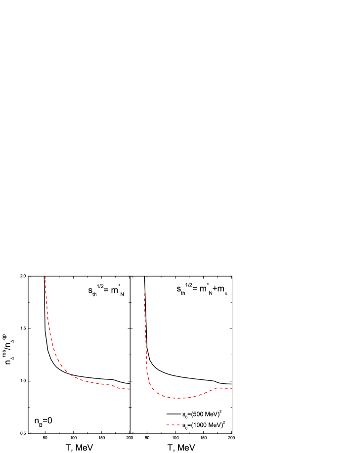
Figure 6: Ratio of the $\Delta$ isobar density, calculated with the inclusion of the width, to that of the quasiparticle one, $R_{\Delta}=n^{\rm res}_{\Delta}/n_{\Delta}^{\rm qp}$, as a function of temperature at $n_{B}=0$ for two values of the resonance threshold energy $s_{th}^{1/2}$. The parameters of calculation are presented in the figure.

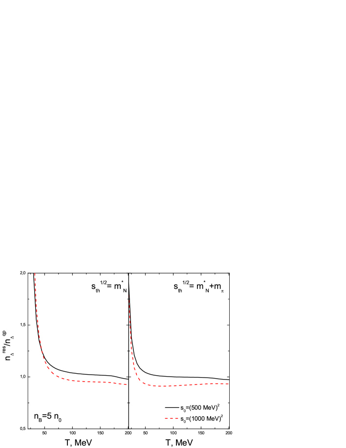
Figure 7: The same as in Fig. 6 but for $n_{B}=5~{}n_{0}$.

In Figs. 6 and 7, we present the ratio $R_{\Delta}=n^{\rm res}_{\Delta}/n_{\Delta}^{\rm qp}$ of the $\Delta$-isobar density, calculated following eq. (54), to the quasiparticle density, as a function of the temperature. The results are presented for the baryon density $n_{B}=0$ (in Fig. 6) and for $n_{B}=5n_{0}$ (in Fig. 7). Our aim here is to demonstrate the effect of a finite particle width. Therefore, instead of searching for the best fit of the spectral function to available experimental data we vary the parameters to show how strongly the density ratio may depend on them. We take into account the $p$-wave nature of the resonance and use $\Gamma_{0}=115~{}$MeV. The threshold quantities are chosen to be $s^{1/2}_{th}=m_{N}^{*}$ (left panels) and $s^{1/2}_{th}=m_{N}^{*}+m_{\pi}$ (right panels). In vacuum $s_{\rm th}^{1/2}=m_{N}+m_{\pi}$. Thus, taking $s_{\rm th}^{1/2}=m^{*}_{N}+m_{\pi}$ we simulate the vacuum resonance placed in the mean field (in our model $m_{\pi}^{*}=m_{\pi}$). With $s_{\rm th}^{1/2}=m^{*}_{N}$ we simulate the effect of in-medium off-shell pions (virtual pions can be produced in matter at any energy). The form factor $F$ is computed with $\beta=3$ and $s_{0}=(500~{}\mbox{MeV})^{2}$ (solid lines) and $s_{0}=(1000~{}\mbox{MeV})^{2}$ (dash lines) to present the dependence of $R_{\Delta}$ on the high-energy behavior of the width, which is not well defined even in vacuum.

As we can see, in all examples the curves are rather flat in the temperature range $T\stackrel{{\scriptstyle\scriptstyle>}}{{\phantom{}{}_{\sim}}}50$ MeV$\div 100$ MeV. For $n_{B}=0$, at $T\simeq 170~{}$MeV there appears a slight bend associated with a sharp decrease in the nucleon effective mass for $T\stackrel{{\scriptstyle\scriptstyle>}}{{\phantom{}{}_{\sim}}}170~{}$MeV. For $n_{B}=5~{}n_{0}$ the bend is smeared. A substantial deviation of the $R_{\Delta}$ ratio from unity for $T\stackrel{{\scriptstyle\scriptstyle>}}{{\phantom{}{}_{\sim}}}50$ MeV$\div 100$ MeV in the case with the cut-off $s_{0}=(1000~{}\mbox{MeV})^{2}$ is due to a larger width at high resonance energies (for large $s$) compared to the case with the cut-off $s_{0}=(500~{}\mbox{MeV})^{2}$. In the latter example, the quasiparticle approximation becomes appropriate for $T\stackrel{{\scriptstyle\scriptstyle>}}{{\phantom{}{}_{\sim}}}100$ MeV. On the contrary, for $s_{0}=(1000~{}\mbox{MeV})^{2}$ and $n_{B}=0$ the quasiparticle approximation does not work at all. For low temperatures, the $R_{\Delta}$ ratio is significantly higher than unity and for higher temperatures it becomes essentially smaller than unity. The broader the width distribution is, the smaller $R_{\Delta}$ at large temperatures. The ratio dependence on the threshold value $s^{1/2}_{th}=m_{N}^{*}$ is rather pronounced for $s_{0}=(1000~{}\mbox{MeV})^{2}$ but it is only minor for $s_{0}=(500~{}\mbox{MeV})^{2}$. Thus, we conclude that taking into account the energy dependence of the width might be quite important for very broad resonances, when the width only slowly decreases with energy. If the width drops rather rapidly with the energy increase, the quasiparticle approximation becomes appropriate for calculation of thermodynamic quantities already at not too high temperature. The baryon density dependence of the ratio $R_{\Delta}$ is not so pronounced (especially for $s_{0}=(500~{}\mbox{MeV})^{2}$), since in our parameterization the spectral function depends on the density only through the value $m^{*}_{\rm r}(n_{B})$ and the choice of $s_{\rm th}$. For low temperatures ($T\stackrel{{\scriptstyle\scriptstyle<}}{{\phantom{}{}_{\sim}}}50\div 100$ MeV), the $R_{\Delta}$ ratio becomes significantly larger than unity. We also pay attention to the shift of the reaction thresholds due to the dependence of the width on $s$ and the threshold $s_{\rm th}$ on the density and temperature. This point can be very important for fitting of particle momentum distributions.

To demonstrate the effect of the finite resonance width on thermodynamic characteristics of the system, we calculate the energy density of the non-interacting resonances (however with width). Then

$$E^{\rm f}_{\rm r}=N_{\rm r}\int_{0}^{\infty}\frac{4\pi p^{2}dp}{(2\pi)^{3}}\int_{0}^{\infty}\frac{ds}{4\pi}\omega\widetilde{A}_{\rm r}f^{\rm f}_{\rm r}+(\mu_{\rm r}\rightarrow-\mu_{\rm r}),$$ (61)

where the degeneracy factor for $\Delta$ is $N_{\rm r}=16$.

In Figs. 8 and 9, we show the ratios of the energy density for $\Delta$’s (with and without width) to the total baryon energy density at $n_{B}=0$ and $n_{B}=5~{}n_{0}$, respectively. The solid and dashed curves correspond to calculational results for the width with $s_{0}=(500~{}\mbox{MeV})^{2}$ and $s_{0}=(1~{}\mbox{GeV})^{2}$. The dash-dotted curve is computed within the quasiparticle approximation. Calculations are performed for two values of the threshold energies $s^{1/2}_{\rm th}=m_{N}^{*}$ (left panels) and $s^{1/2}_{\rm th}=m_{N}^{*}+m_{\pi}$ (right panels).

As was expected, in all cases the quasiparticle result is much closer to that for $s_{0}=(500~{}\mbox{MeV})^{2}$ than for $s_{0}=(1~{}\mbox{GeV})^{2}$. In the former case, the differences are almost negligible. For $s_{0}=(1~{}\mbox{GeV})^{2}$ the ratio remains smaller than the quasiparticle result, except for low temperatures. Differences in the ratios with and without taking into account the width in all cases are not too noticeable. The density dependence of the ratio proves to be pronounced even in our model, although the density dependence of the width is not incorporated explicitly. Summarizing, for calculation of thermodynamic characteristics, one may use the quasiparticle approximation for baryons in the whole temperature interval under consideration provided the high energetic tail of the resonance width-function is not too long. If a resonance has a long energetic tail, then the longer the width tail is, the more suppressed the ratio of the resonance energy to the total energy, as compared to the corresponding quasiparticle ratio.

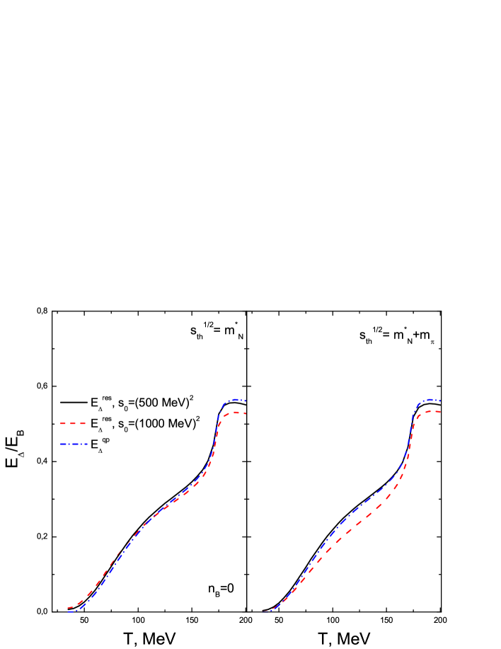
Figure 8: Ratio of the $\Delta$ isobar energy density, calculated with the inclusion of the width ($E_{\Delta}$), to the total baryon energy density ($E_{B}$), as a function of temperature at $n_{B}=0$ for two values of the resonance threshold energy $s_{th}^{1/2}$. The parameters of calculation are presented in the figure. $E^{qp}_{\Delta}$ is calculated within the quasiparticle approximation.

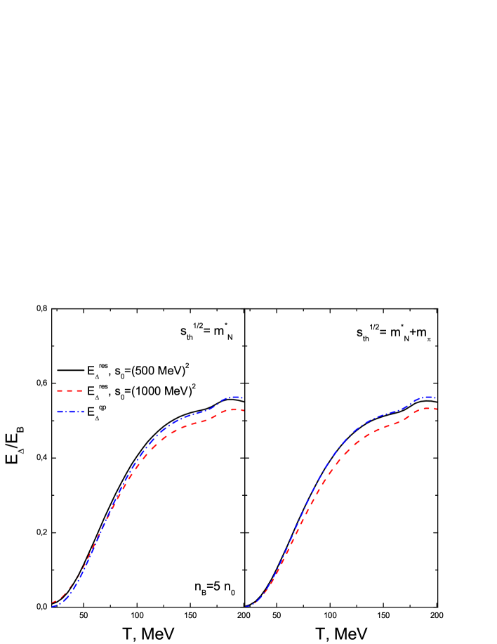
Figure 9: The same as in Fig. 8 but for $n_{B}=5n_{0}$.

For charged bosons the spectral function follows the sum-rule, cf. [45],

$$\int_{0}^{\infty}\frac{ds}{2\pi}A^{\rm b}_{\rm r}=1.$$ (62)

We again consider a dilute matter assuming that the spectral function depends only on the $s$-variable. Only in this case one may consider a single spectral function for vector mesons, like $\omega$ and $\rho$, whereas in the general case one should introduce transversal and longitudinal components.

The Noether charged boson density (of given charge) is given by

$$n^{\rm b}_{\rm r}=(2s_{\rm r}+1)\int_{0}^{\infty}\frac{4\pi p^{2}dp}{(2\pi)^{3}}\int_{0}^{\infty}\frac{d\omega}{2\pi}2\omega\ A^{\rm b}_{\rm r}\ f^{\rm b}_{\rm r},\quad f^{\rm b}_{\rm r}=\frac{1}{e^{(\omega-\mu_{\rm r}^{*})/T}-1}.$$ (63)

For practical calculations it is convenient to present the spectral function in the form:

$$A^{\rm b}_{\rm r}=\frac{\xi\ [\Gamma_{\rm r}^{\rm b}(s)]}{(s-m^{*2}_{\rm r})^{2}+[\Gamma_{\rm r}^{\rm b}(s)]^{2}/4}+\xi\cdot 2\pi\delta(s-(m_{\rm r}^{*})^{2})\ \theta(s_{\rm th}-(m_{\rm r}^{*})^{2})$$ (64)

with $\xi=const$ introduced to fulfill the sum-rule. Replacing $\widetilde{\Gamma}_{\rm r}(s)=\frac{1}{2}\Gamma_{\rm r}^{\rm b}(s)$, we may use eq. (57) for $\widetilde{\Gamma}_{\rm r}(s)$ with $\alpha=1/2$ for $s$ and $\alpha=3/2$ for the $p$ resonance.

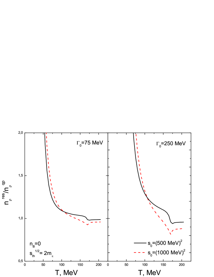
Figure 10: Ratio of the $\rho$ meson density calculated with the inclusion of the width to the quasiparticle one, $R_{\rho}=n^{\rm res}_{\rho}/n_{\rho}^{\rm qp}$, as a function of the temperature at $n_{B}=0$. The parameters of calculation are presented in the figure.

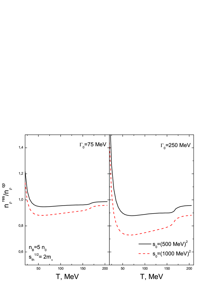
Figure 11: The same as in Fig. 10 but for $n_{B}=5~{}n_{0}$.

In Figs. 10 and 11, the ratio $R_{\rho}=n_{\rho}/n^{\rm qp}_{\rho}$ of the $\rho^{+}$ density, calculated following eq. (63), to the quasiparticle density is shown as a function of the temperature. Here we take into account the $p$-wave nature of the resonance and use two values for the width: a small width $\Gamma_{0}=75~{}$MeV (left panels) and a very large one $\Gamma_{0}=250~{}$MeV (right panels). We use $s_{\rm th}^{1/2}=2m_{\pi}$, thus taking $m_{1}^{*}=m_{2}^{*}=m_{\pi}$. The results are presented for $n_{B}=0$ and $n_{B}=5~{}n_{0}$ in Figs. 10 and 11, respectively. These figures show only a moderate dependence of the ratios $R_{\rho}$ on the value of the width at the resonance peak (on $\Gamma_{0}$). At high energies the energy dependence of the width is more pronounced (compare solid and dash curves). In our model the density dependence of $R_{\rho}$ reflects the behavior of $m^{*}_{\rho}(n_{B})$. For $n_{B}=0$ the ratio $R_{\rho}$ becomes larger than unity for $T\stackrel{{\scriptstyle\scriptstyle<}}{{\phantom{}{}_{\sim}}}100$ MeV, whereas for $n_{B}=5~{}n_{0}$ $R_{\rho}$ is larger than unity only for $T\stackrel{{\scriptstyle\scriptstyle<}}{{\phantom{}{}_{\sim}}}20\div 50$ MeV. The ratio $R_{\rho}(n_{B}=5~{}n_{0})<R_{\rho}(n_{B}=0)$ since the resonance mass $m^{*}_{\rho}(n_{B})$ for $n_{B}=5~{}n_{0}$ is closer to the threshold value $2m_{\pi}$ than in the case of $n_{B}=0$.

Slight bends of the curves at $T\sim 170$ MeV are associated with dropping of the effective mass of $\rho$ below the threshold. Then there arises a quasiparticle contribution to the spectral function being added to the high-energy width term (second term in (64)). In general, the behavior of $R_{\rho}$ and $R_{\Delta}$ is similar. The quasiparticle approximation is rather appropriate for $T\stackrel{{\scriptstyle\scriptstyle>}}{{\phantom{}{}_{\sim}}}100$ MeV, provided the widths have not too long high-energy tails (see curves with $s_{0}^{1/2}=500$ MeV). Under these conditions our quasiparticle SHMC model works well. If the resonance width has a very broad high-energy tail (see curves with $s_{0}^{1/2}=1000$ MeV), the deviation of the $R_{\rm r}$ ratio (for the ${\rm r}$-resonance) from unity is rather pronounced, even for $T\stackrel{{\scriptstyle\scriptstyle>}}{{\phantom{}{}_{\sim}}}100$ MeV. Since in this case $R_{\rm r}<1$, when broad resonances are included, there may appear a possibility to match the lattice data for $T\stackrel{{\scriptstyle\scriptstyle>}}{{\phantom{}{}_{\sim}}}170$ MeV even without suppressing the coupling constants. The latter procedure was used in [6] to demonstrate a possibility to fit the lattice results within our quasiparticle SHMC model.

Broad hadronic resonances having a short lifetime are of a particular interest for dynamics at the late stage of relativistic heavy-ion collisions. As the system expands and cools, it will hadronize and chemically freeze out (vanishing inelastic collisions, no creation of new particles). After some period of hadronic elastic interactions, the system reaches the kinetic freeze out stage, when all hadrons stop interacting at all (vanishing even elastic collisions). After the stage of the kinetic freeze out, particles overcoming remaining mean fields free-stream towards the detectors, where measurements are performed. The lifetimes of the $\rho$ meson and $\Delta$-baryon are $\tau_{\rho}\simeq 1/\Gamma_{0\rho}\simeq 1.3~{}fm/c$ and $\tau_{\Delta}\simeq 1.7~{}fm/c$, respectively, being small with respect to the lifetime of the expanding system. So short-lived resonances can decay and regenerate in scattering process all the way through the kinetic freeze out. The regeneration process depends on the hadronic cross sections of resonance daughters. Thus the study of different resonances can provide an important probe of the time evolution of the source from the beginning of the chemical freeze out to the kinetic one. In-medium effects can modify properties of hadron quasiparticles and resonances during this stage. In particular, it concerns finite widths and energy-momentum relation evolving in time. Values of chemical potentials and the temperature characterizing particle momentum distributions become completely frozen at the kinetic freeze out. From this moment only the mean fields can survive and the hadron effective masses further evolve towards the bare masses with which particles reach detectors.

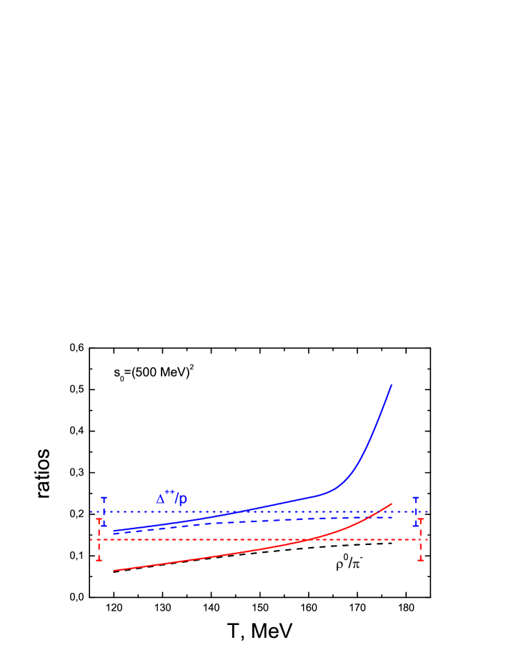
Figure 12: The resonance ratios as a function of temperature. The solid lines are calculated within the SHMC model with accounting for the resonance width according to eqs. (54), (58). Parameters are the same as in Figs. 6 and 10 (right panels, solid lines). The dashed lines are calculated for the IG model. These results are obtained at $\mu_{B}=20$ MeV for the RHIC energy. Experimental data [48] for central $d+Au$ collisions are plotted by straight dotted lines with error bars.

In Fig. 12 the ratios of yields of resonances to the yields of stable particles with similar quark content, the $\rho^{0}/\pi^{-}$ and $\Delta^{++}/p$ ratios, are presented as a function of temperature. For all four species considered, our calculations take into account the feed-down from higher resonances $n^{feed}_{i}=n_{i}+\sum_{r}n_{r}\Gamma^{r\to i}/\Gamma_{r}$. Being in an agreement with experiment, the statistical analysis of stable hadron ratios at the chemical freeze-out [31] shows that these ratios are getting almost energy-independent at $\sqrt{s_{NN}}\stackrel{{\scriptstyle\scriptstyle>}}{{\phantom{}{}_{\sim}}}100$ GeV. This statement seems to be valid also for resonances provided they are treated within the quasiparticle approximation, as follows from the weak $T$ dependence of the ideal gas (IG) model results (see dashed lines in Fig. 12). As is seen in Fig. 12, the resonance ratios calculated in the SHMC and IG models almost coincide with each other till temperature about 140 and 155 MeV for the $\Delta^{++}/p$ and $\rho^{0}/\pi^{-}$ ratios, respectively, and then the difference between them increases with $T$. The growth of the resonance yield in the SHMC model is mainly due to the dropping of the effective mass at high temperatures. Dependence of the resonance abundance on the value of the width and other parameters (at the same temperature) is rather moderate (compare the solid and dashed curves in Figs. 6 and 10).

Earlier, the resonance statistical treatment has been considered in refs. [46] and [47]. Both models are ideal gas ones but in the hadronization statistical model [47] the vacuum (energy independent) resonance widths are included. At the same values $T,\mu_{B}$ these models provide quite close results but if one refers to the particular collision energy, their results differ due to making use of different approximations for the freeze out $T$ and $\mu_{B}$ as functions of the collision energy (see Fig. 5). In the hadronization statistical model [47], predictions were made only for the SPS energies.

Very recently the short-lived resonances $\Delta^{++}$ and $\rho^{0}$ have been measured by the STAR Collaboration at RHIC in $d+Au$ collisions [48]. The observed $\rho^{0}/\pi^{-}$ and $\Delta^{++}/p$ ratios practically do not depend on the charged particle number at the mid rapidity, $dN_{ch}/d\eta$ (i.e. on centrality), and for central ($20\%$ centrality) collisions are $0.139\pm 0.050$ and $0.206\pm 0.034$, respectively [48]. As is seen in Fig. 12, calculated results for the SHMC model cross the experimental line at $T\sim 145$ and $\sim 160$ MeV for $\Delta^{++}/p$ and $\rho^{0}/\pi^{-}$, respectively. However, large experimental error bars do not allow to make preference to any specific model, though the IG model predictions are slightly but regularly below that for the SHMC model. One should remind that at the RHIC energy the chemical freeze out temperature is estimated as 177 MeV [47, 48] and kinetic one is about 120 MeV. The $\rho^{0}/\pi^{-}$ ratio was also measured in peripheral $Au+Au$(200 GeV) collisions [49] to be as large as $\rho^{0}/\pi^{-}=0.169\pm 0.003(stat)\pm 0.027(syst)$. Note that the existence of the difference between the experimental value of $\rho^{0}/\pi^{-}$ ratio and the statistical model result has been considered as a problem in ref. [47]. Following their estimate, $\rho^{0}/\pi^{-}$ ratio is about $4\cdot 10^{-4}$ at the kinetic freeze out temperature 120 MeV, and it is 0.11 at the chemical freeze out $T=177$ MeV. Our result ($\sim 0.06$ at $T=120$ MeV) strongly deviates from the statistical estimate [47] at the kinetic freeze out. At the chemical freeze out temperature, $T=177$ MeV, predictions of the $\rho^{0}/\pi^{-}$ ratio practically coincide in all ideal gas based models remaining lower than the experimental ratio, whereas our SHMC model is able to reproduce experiment at $T\sim 165\div 170$ MeV. It is also of interest that the measured resonances have a mass shift about 50-70 MeV  [48] which is consistent with the SHMC model results at $T\sim 160$ MeV as presented in Fig. 2. Thus, one may infer that due to a possible decay, regeneration and rescattering, the broad resonances, if they are treated within the statistical picture with taken into account their in-medium mass shift, freeze at a somewhat lower temperature than that at the chemical freeze out but this temperature is significantly higher than the value of $T\approx 120$ MeV, characterizing the kinetic freeze out [50]. A dynamical consideration of the freeze out is needed to draw more definite conclusions.

5 Concluding remarks

In this paper we made attempts to find several improvements of the SHMC model of [6].

In [6] the boson excitation effects were assumed to be small. Therefore their contribution to thermodynamic characteristics was calculated using perturbation theory in the fields of boson excitations. Thereby, boson excitation contributions in the equations of motion were dropped. The approximation made needs justification. Here we incorporated the boson excitation terms in the equations of motion and then calculated thermodynamic quantities (including boson excitation parts). Corrections to the effective masses of the $\sigma$, and $\omega$-$\rho$-nucleon excitations turn to be minor for $T\stackrel{{\scriptstyle\scriptstyle<}}{{\phantom{}{}_{\sim}}}100\div 120$ MeV and grow with the temperature increase. Corrections to thermodynamic characteristics, like total pressure, energy, entropy etc., remain moderate even at higher temperatures. Qualitatively, one may conclude that all results of [6] remained unchanged. With boson excitation terms incorporated into the equations of motion, our quasiparticle SHMC model fulfills exactly the thermodynamic consistency conditions.

Then we discussed possible effects of the resonance widths. We assumed vacuum but energy-dependent widths of resonances. Under this assumption the width effects included do not change qualitative behavior of the system. Nevertheless, one should note that in dense and/or hot matter particle widths may acquire essential density- and temperature-dependent contributions that may significantly affect properties of the system, e.g., see [42], where for the case of hot baryon-less system it is shown that width effects may completely smear fermion distributions. We illustrated that the estimated yields of short-lived resonances to be important for the late stage of relativistic heavy-ion collisions can be described sufficiently well if one treats those resonances in the framework of our SHMC model with the vacuum widths at the freeze out.

In the paper, the $\sigma$ variable was considered as an order parameter. Then the effective masses of $\sigma^{{}^{\prime}}$, $\omega^{{}^{\prime}}$, $\rho^{{}^{\prime}}$ excitations and the effective masses of nucleons have a similar behavior as a function of the baryon density and temperature. The effective masses remain rather flat functions of the temperature and sharply drop to zero only in the vicinity of $T_{c}$. In the large temperature interval mentioned, the effective masses as a function of the density first decrease with the density increase and then, at a very high density, begin to grow, cf. [6].

In Appendix A we calculated what modifications of our model could be, if the $\sigma$-$\omega$ and $\rho$ fields were treated on equal footing. In the latter case, the density-temperature behavior of the $\sigma^{{}^{\prime}}$ excitation mass essentially differs from that of the $\omega^{{}^{\prime}}$-$\rho^{{}^{\prime}}$ excitation masses, namely, the $\sigma^{{}^{\prime}}$ excitation mass drops to zero at $n_{c}\simeq 4.2~{}n_{0}$ and only slightly depends on $T$. Thus, if this model was applied to analyze heavy ion collisions, we would face with a problem of Bose condensation of $\sigma^{{}^{\prime}}$ excitations for $n_{B}>n_{c}\sim 4\div 5~{}n_{0}$ in a broad temperature interval. Another unpleasant feature of a model version like this is a drastic difference in the density behavior of the $\sigma^{{}^{\prime}}$ effective mass and that of $\omega^{{}^{\prime}}$-$\rho^{{}^{\prime}}$ excitations. These are additional arguments in favor of the treatment of the $\sigma$ variable as an order parameter (as we did earlier in ref. [6] and here in the paper body).

Then in Appendix B an attempt was made to incorporate the nucleon-nucleon hole and nucleon-antinucleon loop effects in our model. The loop terms mentioned were calculated within the perturbative approach. If these terms are taken into account, the $\sigma^{{}^{\prime}}$ excitation effective mass exhibits rather unrealistic behavior. Thus, the model completely loses its attractiveness if baryon loops are included (at least within the perturbative approach). We have checked that this unpleasant feature is a common feature of many RMF models, including the original Walecka model (previously authors of ref. [51] arrived at a similar conclusion considering vacuum loop corrections in the Walecka model). In the Fermi liquid approach to diminish contribution of the fermion loop terms one incorporates the vertices corrected by a short-range baryon-baryon interaction introduced with the help of the Landau-Migdal parameters, cf. [24, 25, 26]. In the framework of our SHMC model short-range correlation effects are simulated by the $\omega$, $\sigma$, $\rho$ exchanges and are non-local. Thereby, we do not include these effects in the present work. Summarizing, either higher order fluctuation effects should be included in all orders, that is a complicated problem, or they should be skipped within RMF based models. So we skipped these terms in our truncated scheme.

Concluding, the SHMC model introduced in ref. [6] can be considered as a reasonable model for application to the description of hadronic matter in a broad baryon density-temperature range, provided higher order fluctuations of fermion fields are not included.

Acknowledgements

We are very grateful to A. Andronic, Yu.B. Ivanov, E.E. Kolomeitsev, K. Redlich, and V.V. Skokov for numerous illuminating discussions, valuable remarks, and constructive criticism. This work was supported in part by the Deutsche Forschungsgemeinschaft (DFG project 436 RUS 113/558/0-3), and the Russian Foundation for Basic Research (RFBR grants 06-02-04001 and 08-02-01003).

Appendix A. Treatment of the $\sigma$ field as an independent variable. As noted in the paper, we continue to suppress contributions of baryon loops. If the $\sigma$ and $\omega_{0}$ fields are treated on equal footing, i.e. as independent variables (”ind.var.”), one can determine the effective $\sigma^{{}^{\prime}}$-mass using partial derivatives of the pressure,

$$(m_{\sigma}^{\rm part*})^{2}_{\rm ind.var.}=-\frac{{\partial^{2}\sum_{m\in\{m\}}P_{m}^{\rm MF}[f,\omega_{0}]}}{{\partial f^{2}}}\left(\frac{df}{d\sigma}\right)^{2},$$ (65)

rather than full derivatives.

It is convenient to present

$$\frac{{d^{2}\sum_{m\in\{m\}}P_{m}^{\rm MF}[f,\omega_{0}(f)]}}{{df^{2}}}=\frac{{\partial^{2}\sum_{m\in\{m\}}P_{m}^{\rm MF}[f,\omega_{0}]}}{{\partial f^{2}}}+\delta_{\sigma},$$

$$\delta_{\sigma}\simeq\frac{\partial^{2}\sum_{m\in\{m\}}P_{m}^{\rm MF}}{\partial\omega_{0}^{2}}\left(\frac{\partial\omega_{0}}{\partial f}\right)^{2}+2\frac{\partial^{2}\sum_{m\in\{m\}}P_{m}^{\rm MF}}{\partial\omega_{0}\partial f}\frac{\partial\omega_{0}}{\partial f}.$$ (66)

Taking derivatives in (65) and (5) we use the exact equation of motion for $f$ and $\omega_{0}$, and suppress the boson excitation and baryon-loop contributions to the pressure in the final expression.

Taking partial derivatives we get

$$-\frac{{\partial^{2}\sum_{m\in\{m\}}P_{m}^{\rm MF}[f,\omega_{0}]}}{{\partial f^{2}}}\simeq\frac{m^{4}_{N}}{C_{\sigma}^{2}}+U^{\prime\prime}_{f}-\omega_{0}^{2}m_{\omega}^{2},$$ (67)

and $\delta_{\sigma}=-\omega_{0}^{2}m_{\omega}^{2}$, where $\eta_{\sigma}=1$ was used.

If the effective $\sigma^{{}^{\prime}}$-excitation mass squared is determined using the Hamiltonian we obtain

$$\left<\frac{{\partial^{2}H[f,\omega_{0}]}}{{\partial f^{2}}}\right>=\frac{m^{4}_{N}}{C_{\sigma}^{2}}+U^{\prime\prime}_{f}-\omega_{0}^{2}m_{\omega}^{2}+\omega_{0}\frac{\partial^{2}\chi_{\omega}}{\partial f^{2}}\sum_{b\in\{b\}}g_{\omega b}t_{b}n_{b},$$ (68)

that differs from (67) by the last term.

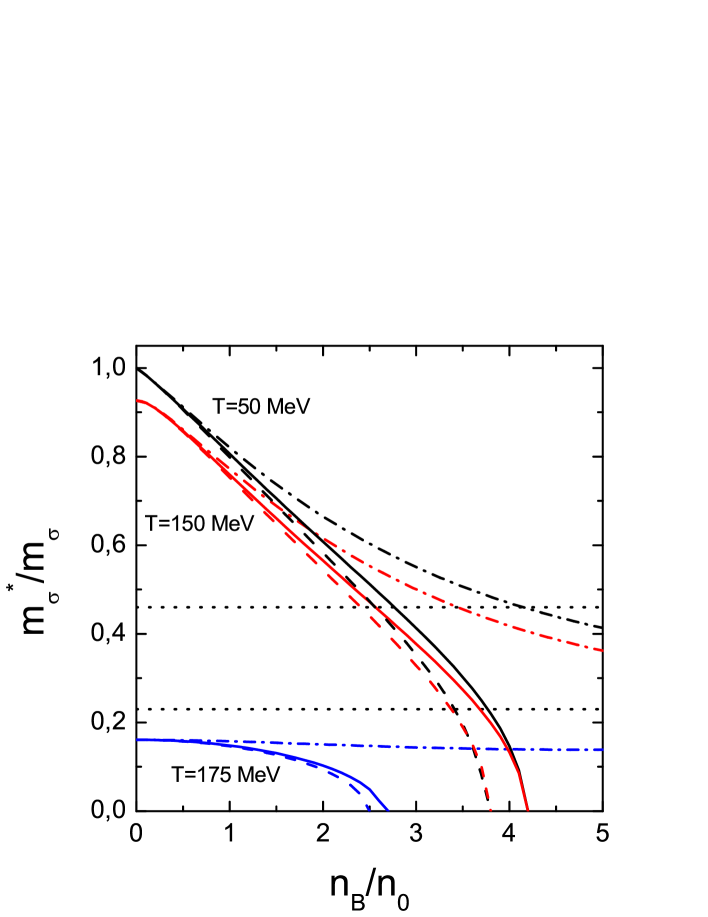
Figure 13: The effective $\sigma^{{}^{\prime}}$ excitation mass as a function of density calculated using eqs. (65) (solid curves), (68) (dash lines), and (42) (dash-dotted curves) for different temperatures. Straight dotted lines correspond to $m_{\sigma}=2m_{\pi}$ and $m_{\sigma}=m_{\pi}$.

In Fig.13, we show the ratio of the effective-to-bare masses of the $\sigma^{{}^{\prime}}$ excitation as a function of the baryon density at different values of the temperature for two possible treatments of the $\sigma$-field, as an order parameter, see (42), and as an independent variable. In the latter case two expressions, (65) and (68), were used to calculate the value $m_{\sigma}^{\rm part*}$. The solid lines are evaluated following eq.(65) for $T=50,\ 150$ and $175$ MeV (from the top to the bottom); and the dashed curves, using (68). In both the cases the effective $\sigma^{{}^{\prime}}$ excitation mass, calculated following (65), drops to zero at $n_{B}\approx 4.2n_{0}$ (for $T=50$ MeV) and for $n_{B}\approx 3.8~{}n_{0}$ (for $T=150$ MeV), respectively, which demonstrates a moderate temperature dependence of the effective mass up to $T\sim 150~{}$MeV. For higher temperatures the critical density significantly decreases. In all the cases, the differences between calculations following (65) and (68) are minor; however, they significantly deviate from calculational results following eq. (42) (dash-dotted curves). The behavior of the effective $\sigma^{{}^{\prime}}$ excitation mass calculated using (65) and (68) is in contrast with the behavior of the $\omega^{{}^{\prime}}$-$\rho^{{}^{\prime}}$-$N$ effective masses which do not reach zero for all densities (see dash-dotted curves). Since one of our main goals was to construct a model based on the idea of a rather similar behavior for all $\sigma^{{}^{\prime}}$-$\omega^{{}^{\prime}}$-$\rho^{{}^{\prime}}$-$N$ excitation masses, we refuse considering the $\sigma$ field, as an independent variable, i.e., we refuse to consider it on equal footing with the $\omega$ and $\rho$ fields. Therefore, instead of either eq. (65) or eq. (68), here we use eq. (42) treating the $\sigma$ field as an order parameter.

Appendix B. Inclusion of baryon loops.

In the general case, the $\sigma^{{}^{\prime}}$ excitation mass is given by eq. (39), provided the $\sigma$ field is treated as an order parameter. We will continue to keep only quadratic terms in fluctuating boson fields. Thus, we drop the boson excitation term in the pressure in expression (39) but we will keep the baryon term. So in contrast with (42), we use the expression

$$(m_{\sigma}^{\rm part*})^{2}\simeq - \left[\frac{{d^{2}\sum_{m\in\{m\}}P_{m}^{\rm MF}[f,\omega_{0}(f)]}}{{df^{2}}}\right.$$ (69)

$$+ \left.\frac{{d^{2}\sum_{b\in\{b\}}P_{b}[f,\omega_{0}(f)]}}{{df^{2}}}\right]\left(\frac{df}{d\sigma}\right)^{2}.$$

An important difference between (69) and (45) (the latter expression yields the same result as (42)) is that derivatives of the Hamiltonian are taken at fixed $\Psi_{B}$, whereas the total pressure $P$ depends on the baryon occupations, which should be varied. Thereby, (69) includes extra contributions from the baryon-baryon hole and baryon-antibaryon excitations.

Let us now calculate an additional, purely baryon contribution to the $\sigma^{{}^{\prime}}$-excitation mass incorporated in (69). Using that

$$\frac{\partial f_{b}}{\partial f}=\frac{\partial f_{b}}{\partial\omega_{b}}\left[\frac{\partial\omega_{b}}{\partial f}+g_{\omega b}\omega_{0}\frac{\partial\chi_{\omega}}{\partial f}\right],\quad\frac{\omega_{b}}{p}\frac{\partial f_{b}}{\partial p}=\frac{\partial f_{b}}{\partial\omega_{b}},$$ (70)

and (26), with the help of partial differentiations we find

$$\delta_{B}(m_{\sigma}^{\rm part*})^{2}=-\left(\frac{df}{d\sigma}\right)^{2}\sum_{b\in\{b\}}\frac{{\partial^{2}P_{b}[f,\omega_{0}]}}{{\partial f^{2}}},$$

$$-\sum_{b\in\{b\}}\frac{{\partial^{2}P_{b}[f,\omega_{0}]}}{{\partial f^{2}}}=m_{N}^{2}\sum_{b\in\{b\}}x_{\sigma b}^{2}\left[\frac{2n_{sb}}{m_{b}^{*}}-L_{b}\right]+\sum_{b\in\{b\}}g_{\omega b}\omega_{0}\ t_{b}\ n_{b}\ \frac{\partial^{2}\chi_{\omega}}{\partial f^{2}}$$

$$-\sum_{b\in\{b\}}\left(g_{\omega b}\omega_{0}\frac{\partial\chi_{\omega}}{\partial f}\right)^{2}B_{b}+2m_{N}\sum_{b}x_{\sigma b}g_{\omega b}\omega_{0}\frac{\partial\chi_{\omega}}{\partial f}\widetilde{L}_{b}.$$ (71)

We also use the equations of motion and the relation $\left(\frac{\partial m_{b}^{*}}{\partial f}\right)=-x_{\sigma b}m_{N}$.

Here the quantities

$$B_{b}=L_{b}+\frac{n_{sb}}{m_{b}^{*}},$$ (72)

and

$$L_{b}=N_{b}\ \int_{0}^{\infty}\frac{dp}{2\pi^{2}}\ \omega_{b}\ f_{b}$$ (73)

are the baryon-baryon hole and baryon-antibaryon loop-terms taken at zero incoming energy and momentum.

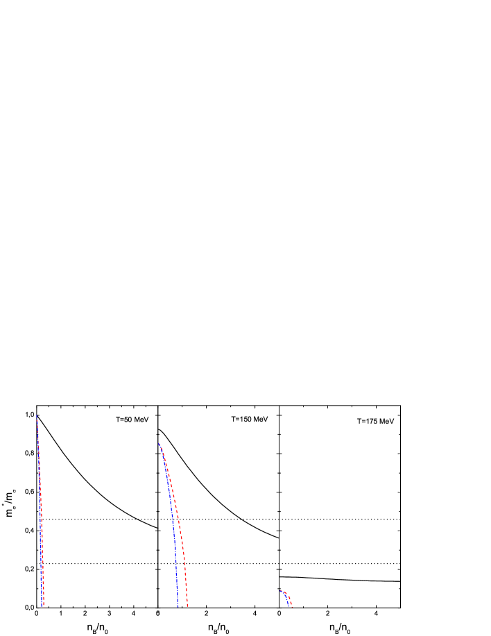
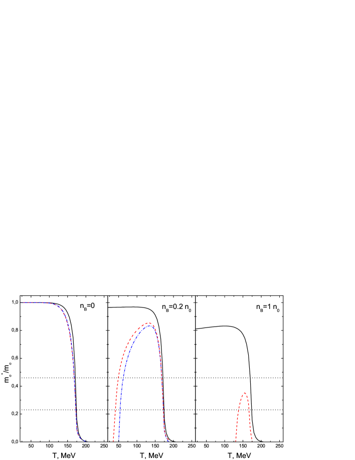
Figure 14: The ratio of the effective $\sigma^{\prime}$ excitation mass to the bare mass as a function of density (top) and temperature (bottom) calculated by means of eqs. (42), (solid curves), eq. (78) (dashed curves) and eq. (77) (dash-dotted lines), see (69). The straight dotted lines correspond to the level of $m_{\sigma}=2m_{\pi}$ and $m_{\sigma}=m_{\pi}$.

We also introduce a similar quantity

$$\widetilde{L}_{b}=N_{b}\ \int_{0}^{\infty}\frac{dp}{2\pi^{2}}m_{b}^{*}\ t_{b}\ f_{b}.$$ (74)

Then we calculate an additional contribution

$$\delta=-\frac{{d^{2}P[f,\omega_{0}(f)]}}{{df^{2}}}+\frac{{\partial^{2}P[f,\omega_{0}]}}{{\partial f^{2}}}$$

$$=(m_{\omega}^{part*.0})^{2}\left(\frac{\partial\omega_{0}}{\partial f}\right)^{2}+2\left[m_{\omega}^{2}\omega_{0}\frac{\partial{\Phi_{\omega}}^{2}}{\partial f}-\sum_{b\in\{b\}}g_{\omega b}\ t_{b}\ n_{b}\frac{\partial\chi_{\omega}}{\partial f}\right.$$

$$\left.+\chi_{\omega}\omega_{0}\frac{\partial\chi_{\omega}}{\partial f}\sum_{b\in\{b\}}g_{\omega b}^{2}\,B_{b}-m_{N}\chi_{\omega}\sum_{b\in\{b\}}g_{\omega b}x_{\sigma b}\widetilde{L}_{b}\,\right]\frac{\partial\omega_{0}}{\partial f},$$ (75)

that distinguishes full and partial derivative terms. Here

$$\frac{\partial\omega_{0}}{\partial f}\left[1+\sum_{b\in\{b\}}\frac{g_{\omega b}^{2}}{m_{\omega}^{2}\eta_{\omega}}B_{b}\right]=\sum_{b\in\{b\}}\frac{g_{\omega b}}{m_{\omega}^{2}\eta_{\omega}\chi_{\omega}}\left[x_{\sigma b}m_{N}\widetilde{L}_{b}-B_{b}g_{\omega b}\frac{\partial\chi_{\omega}}{\partial f}\,\omega_{0}\right]$$ (76)

$$+ \sum_{b\in\{b\}}\frac{g_{\omega b}\ t_{b}\ n_{b}}{m_{\omega}^{2}}\frac{\partial[\eta_{\omega}\chi_{\omega}]^{-1}}{\partial f}$$

with $(m_{\omega}^{part*.0})^{2}={\partial^{2}P^{\rm MF}}/{\partial\omega_{0}^{2}}$.

In [6], the baryon excitation loop $L_{b}$ contributions were suppressed. On the other hand, one may check that $L_{b}>n_{sb}/m_{b}^{*}$, $L_{b}>\widetilde{L}_{b}$. Therefore, in [6] we disregarded the term $\delta_{B}(m_{\sigma}^{\rm part*})^{2}$ as the whole, as well as the terms $\propto B_{b}$ and $\widetilde{L}_{b}$ in (5) and (76). Thus in [6] eq. (42) is actually used, being compatible with (45).

Incorporating the loop terms mentioned, one should use the following expression

$${{(m_{\sigma}^{\rm part*})^{2}=\left[-\!\!\!\!\sum_{m\in\{m\}}\frac{{{\partial}^{2}P_{m}^{\rm MF}[f,\omega_{0}]}}{{{\partial}f^{2}}}+\delta_{B}(m_{\sigma}^{\rm part*})^{2}+\delta\right]\!\left(\frac{df}{d\sigma}\right)^{2},}}$$ (77)

where partial contributions are given by (67), (5) and (5).

If $\sigma$ and $\omega_{0}$ are treated on equal footing, i.e. as independent variables (”ind.var.”), one should use

$$(m_{\sigma}^{\rm part*})^{2}_{\rm ind.var.}=-\frac{{\partial^{2}P[\sigma,\omega_{0}]}}{{\partial\sigma^{2}}}\simeq-\frac{{\partial^{2}P[f,\omega_{0}]}}{{\partial f^{2}}}\left(\frac{df}{d\sigma}\right)^{2}.$$ (78)

The ratio of effective-to-bare masses of the $\sigma^{{}^{\prime}}$-excitation is shown in Fig. 14 as a function of the baryon density for three values of temperatures (top panel) and as a function of the temperature for three values of the baryon density $n_{B}$ (bottom panel) calculated by means of eq. (77), i.e., following (69). Results are compared with (78) and (42). As we can see, the inclusion of the baryon loop terms (performed within the perturbation theory) completely destroys all achievements of our SHMC model (besides the case $n_{B}=0$ when these loop terms are suppressed).

Thus, at the moment we can see no simple way to generalize the mean field based the SHMC model which would include baryon-antibaryon and baryon – baryon hole fluctuations.

References

- [1] V. Metag, Prog. Part. Nucl. Phys. 61 (2008) 245 [arXiv:0711.4709].
- [2] R. Rapp and J. Wambach, Adv. Nucl. Phys. 25 (2000) 1; R. Rapp, nucl-th/0608022.
- [3] P. Senger, J. Phys. G30 (2004) S1087; Acta Phys. Hung. A22 (2005) 363; Proposal for the International Accelerator Facility for Research with Heavy Ions and Antiprotons, http://www.gsi.de/documents/DOC-2004-Mar-196-2.pdf.
- [4] A.N. Sissakian, A.S. Sorin and V.D. Toneev, In Proceedings of the 33rd International conference on High Energy Physics, Moscow, IHEP’06, Russia, 28 July - 2 August 2006, edited by A. Sissakian, G. Kozlov, E. Kolganova, World Scientific, Vol.1, p.421, 2007 [nucl-th/0608032]; NICA project: http://nica.jinr.ru.
-
[5]
G.S. Stephans, J. Phys. G32: Nucl. Part. Phys.
(2006) S447-S454 [nucl-ex/0607030]; RICEN BNL Research Center
Workshop: Can we discover the QCD critical point at RHIC ?,
March 9-10, 2006,
https:/www.bnl.gov/riken/QCDrhic/. - [6] A.S. Khvorostukhin, V.D. Toneev and D.N. Voskresensky, Nucl. Phys. A791 (2007) 180.
- [7] T. Klähn et al., Phys. Rev. C74 (2006) 035802.
- [8] C. Fuchs, Lect. Notes Phys. 641 (2004) 119.
- [9] E.E. Kolomeitsev and D.N. Voskresensky, Nucl. Phys. A759 (2005) 373.
- [10] V. Koch, Int. J. Mod. Phys. E 6 (1997) 203.
- [11] G.E. Brown and M. Rho, Phys. Rev. Lett. 66 (1991) 2720; Phys. Rep. 396 (2004) 1.
- [12] C. Fuchs, arXiv:0711.3367.
- [13] G.Q. Li, C.M. Ko and G.E. Brown, Nucl. Phys. A606 (1996) 568.
- [14] A. Onishi, N. Kawamoto and K. Miura, arXiv:0803.0255.
- [15] C.J. Horowitz and J. Piekarewicz, Astroph. J. 593 (2003) 463.
- [16] R.J. Furnstahl, B.D. Serot and H.B. Tang, Nucl. Phys. A598 (1996) 539; A615 (1997) 441.
- [17] M. Dey, V.L. Eletsky and B.L. Ioffe, Phys. Lett. B252 (1990) 620.
- [18] M. Lutz and E.E. Kolomeitsev, Found. Phys. 31 (2001) 1671.
- [19] J.D. Walecka, Phys. Lett. B59 (1975) 109.
- [20] R.A. Freedman, Phys. Lett. B71 (1977) 369.
- [21] K. Saito, Tomoyuki Maruyama and K. Soutomi, Phys. Rev., C40 (1989) 407; K. Soutomi, Tomoyuki Maruyama and K. Saito, Nucl. Phys. A507 (1990) 731.
- [22] K. Weber et al., Nucl. Phys. A539 (1992) 713; Nucl. Phys A552 (1993) 571.
- [23] Tomoyuki Maruyama and S. Chiba, Phys. Rev. C61 (2000) 037301; Phys. Rev. C74 (2006) 014315; S. Typel, Phys. Rev. C71 (2005) 064301.
- [24] A.B. Migdal, E.E. Saperstein, M.A. Troitsky and D.N. Voskresensky, Phys. Rept. 192 (1990) 179.
- [25] D.N. Voskresensky, Nucl. Phys. A555 (1993) 293.
- [26] E.E. Kolomeitsev and D.N. Voskresensky, Phys. Rev. C68 (2003) 015803.
- [27] H. Feldmeier and J. Lindner, Z. Phys. A341 (1991) 83.
- [28] C.Y. Wang, A.K. Kerman, G.R. Satchler and A.D. Mackelar, Phys. Rev. C29, (1984) 574; S. Teis, W. Cassing, Tomoyuki Maruyama and U. Mosel, Phys. Rev. C50 (1994) 388; C.J. Batty, E. Friedman and A. Gal, Phys. Rep. 287 (1997) 385.
- [29] X.H. Zhong, G.X. Peng, Lei Li and P.Z. Ning, Phys.Rev. C73 (2006) 015205.
- [30] F. Karsch, E. Laermann and A. Peikert, Nucl. Phys. B605 (2001) 579.
- [31] A. Andronic, P. Braun-Munzinger and J. Stachel, Nucl. Phys. A772 (2006) 167.
- [32] J. Cleymans and K. Redlich, Phys. Rev. Lett. 81 (1998) 5284.
- [33] F. Beccatini, J. Manninen and M. Gazdzicki, Phys. Rev. C73 (2006) 044905.
- [34] S. Ejiri, F. Karsch, E. Laermann and C. Schmidt, Phys. Rev. D73 (2006) 054506; F. Karsch, hep-lat/0601013.
- [35] M. Reiter, A. Dumitru, J. Brachman, J.A. Maruhn, H. Stöcker and W. Greiner, nucl-th/9801068.
- [36] D.N. Voskresensky and A.V. Senatorov, Sov. J. Nucl. Phys., 53 (1991) 935.
- [37] R. Arnaldi et al. (the NA60 Collaboration), Phys. Rev. Lett. 96 (2006) 162302.
- [38] V.V. Skokov and V.D. Toneev, Acta Phys. Slov. 56 (2005) 503; Phys. Rev. C79 021902 (2006).
- [39] G.E. Brown and M. Rho, nucl-th/0509001; nucl-th/0509002.
- [40] J. Ruppert, T. Renk and B. Muller, Phys. Rev. C73 (2006) 034907.
- [41] G.E. Brown et al., arXiv:0804.3196.
- [42] D.N. Voskresensky, Nucl. Phys. A744 (2004) 378.
- [43] L. Jahnke and S. Leupold, Nucl. Phys. A778 (2006) 53.
- [44] Yu.B. Ivanov, J. Knoll and D.N. Voskresensky, Nucl. Phys. A657 (1999) 413; Yu.B. Ivanov, J. Knoll and D.N. Voskresensky, Nucl. Phys. A672 (2000) 313.
- [45] Yu.B. Ivanov, J. Knoll and D.N. Voskresensky, Phys. Atom. Nucl. 66 (2003) 1902.
- [46] F. Becattini et al., Phys. Rev. C69 (2004) 024905.
- [47] P. Braun-Munzinger, K. Redlich and J. Stachel, In ”Quark Gluon Plasma 3”, eds. R. C. Hwa and Xin-Nian Wang, World Scientific Publishing, 2004, p.491.
- [48] B.I. Abelev at al. (STAR Collaboration), arXiv:0801.0450.
- [49] J. Adams at al. (STAR Collaboration), Phys. Rev. Lett. 92 (2004) 092301.
- [50] E.V. Shuryak and G.E. Brown, Nucl. Phys. A717 (2003) 322.
- [51] R.J. Furnstahl, R.J. Perry and B.D. Serot, Phys. Rev. C40 (1989) 321.