GENERALIZED ENTANGLEMENT IN STATIC AND DYNAMIC QUANTUM PHASE TRANSITIONS

Abstract

We investigate a class of one-dimensional, exactly solvable anisotropic XY spin-$1/2$ models in an alternating transverse magnetic field from an entanglement perspective. We find that a physically motivated Lie-algebraic generalized entanglement measure faithfully portraits the static phase diagram – including second- and fourth-order quantum phase transitions belonging to distinct universality classes. In the simplest time-dependent scenario of a slow quench across a quantum critical point, we identify parameter regimes where entanglement exhibits universal dynamical scaling relative to the static limit.

1 Introduction

Developing methodologies for probing, understanding, and controlling quantum phases of matter under a broad range of equilibrium and non-equilibrium conditions is a central goal of condensed-matter physics and quantum statistical mechanics. Since novel forms of matter tend to emerge in the deep quantum regime where thermal effects are frozen out, a key prerequisite is to obtain an accurate theoretical understanding of zero-temperature quantum phase transitions (QPTs) [1]. Aside from its broad conceptual significance, such a need is heightened by the growing body of experimental work which is being performed at the interface between material science, quantum device technology, and experimental implementations of quantum information processing (QIP). Following the experimental realization of the Bose-Hubbard model in a confined ⁸⁷Rb Bose-Einstein condensate and the spectacular observation of the superfluid-to-Mott-insulator QPT [2], ultracold atoms are enabling investigations into strongly interacting many-body systems with an unprecedented degree of control and flexibility – culminating in the observation of topological defects in a rapidly quenched spinor Bose-Einstein condensate [3]. Remarkably, the occurrence of a QPT influences physical properties well into the finite-temperature regime where real-world systems live, as vividly demonstrated by the measured low-temperature resistivity behavior in heavy-fermion compounds [4].

From a theoretical standpoint, achieving as a complete and rigorous quantum-mechanical formulation as desired is hindered by the complexity of quantum correlations in many-body states and dynamical evolutions. Motivated by the fact that QIP science provides, first and foremost, an organizing framework for addressing and quantifying different aspects of “complexity” in quantum systems, it is natural to ask: Can QIP concepts and tools contribute to advance our understanding of many-body quantum systems? In recent years, entanglement theory has emerged as a powerful bridging testbed for tackling this broad question from an information-physics perspective. On one hand, entanglement is intimately tied to the inherent complexity of QIP, by constituting, in particular, a necessary resource for computational speed-up in pure-state quantum algorithms [5]. On the other hand, critically reassessing traditional many-body settings in the light of entanglement theory has already resulted in a number of conceptual, computational, and information-theoretic developments. Notable advances include efficient representations of quantum states based on so-called projected entangled pair states [6], improved renormalization-group methods for both static 2D and time-dependent 1D lattice systems [7], as well as rigorous results on the computational complexity of such methods and the solvability properties of a class of generalized mean-field Hamiltonians [8].

In this work, we focus on the problem of characterizing quantum critical models from a Generalized Entanglement (GE) perspective [9, 10], by continuing our earlier exploration with a twofold objective in mind: first, to further test the usefulness of GE-based criticality indicators in characterizing static quantum phase diagrams with a higher degree of complexity than considered so far (in particular, multiple competing phases); second, to start analyzing time-dependent, non-equilibrium QPTs, for which a number of outstanding physics questions remain. In this context, special emphasis will be devoted to establish the emergence and validity of universal scaling laws for non-equilibrium observables.

2 Generalized Entanglement in a Nutshell

2.1 The need for GE

Because a QPT is driven by a purely quantum change in the many-body ground-state correlations, the notion of entanglement appears naturally suited to probe quantum criticality from an information-theoretic standpoint: What is the structure and role of entanglement near and across criticality? Can appropriate entanglement measures detect and classify quantum critical points (QCPs) according to their universality properties? Extensive investigations have resulted in a number of suggestive results, see e.g. Ref. fazio for a recent review. In particular, pairwise entanglement, quantified by so-called concurrence, has been found to develop distinctive singular behavior at criticality in the thermodynamic limit, universal scaling laws being obeyed in both 1D and 2D systems. Additionally, it has been established that the crossing of a QCP point is typically signaled by a logarithmic divergence of the entanglement entropy of a block of nearby particles, in agreement with predictions from conformal field theory. While this growing body of results well illustrates the usefulness of an entanglement-based view of quantum criticality, a general theoretical understanding is far from being reached. With a few exceptions, the existing entanglement studies have focused on analyzing how (i) bipartite quantum correlations (among two particles or two contiguous blocks) behave near and across a QCP under the assumption that the underlying microscopic degrees of freedom correspond to (ii) distinguishable subsystems (iii) at equilibrium.

GE provides an entanglement framework which is uniquely positioned to overcome the above limitations, while still ensuring consistency with the standard “subsystem-based” entanglement theory in well-characterized limits [9, 10, 12]. Physically, GE rests on the idea that entanglement is an observer-dependent concept, whose properties are determined by the expectations values of a distinguished subspace of observables $\Omega$, without reference to a preferred decomposition of the overall system into subsystems. The starting point is to generalize the observation that standard entangled pure states of a composite quantum system look mixed relative to an “observer” whose knowledge is restricted to local expectation values. Consider, in the simplest case, two distinguishable spin-$1/2$ subsystems in a singlet (Bell) state,

$$|\text{Bell}\rangle=\frac{|\uparrow\rangle_{A}\otimes|\downarrow\rangle_{B}-|\downarrow\rangle_{A}\otimes|\uparrow\rangle_{B}}{\sqrt{2}}\,,$$ (1)

defined on a tensor-product state space ${\mathcal{H}}={\mathcal{H}}_{A}\otimes{\mathcal{H}}_{B}$. First, the statement that $|\text{Bell}\rangle$ is entangled – $|\text{Bell}\rangle$ cannot be expressed as $|\psi\rangle_{A}\otimes|\varphi\rangle_{B}$ for arbitrary $|\psi\rangle_{A}\in{\mathcal{H}}_{A}$, $|\varphi\rangle_{B}\in{\mathcal{H}}_{B}$ – is unambiguously defined only after a preferred tensor-product decomposition of ${\mathcal{H}}$ is fixed: Should the latter change, so would entanglement in general [12]. Second, the statement that $|\text{Bell}\rangle$ is entangled is equivalent to the property that (either) reduced subsystem state – as given by the partial trace operation, $\rho_{A}=\text{Tr}_{B}\{|\text{Bell}\rangle\langle\text{Bell}|\}$ – is mixed, $\text{Tr}\{\rho_{A}^{2}\}=1/2(1+\sum_{\alpha=x,y,z}\langle\sigma_{\alpha}^{A}\rangle^{2})<1$, in terms of expectations of the Pauli spin-$1/2$ matrices $\sigma_{\alpha}^{A}$ acting on $A$.

To the purposes of defining GE, the key step is to realize that a meaningful notion of a reduced state may be constructed for any pure state $|\psi\rangle\in{\mathcal{H}}$ without invoking a partial trace, by specifying such a reduced “$\Omega$-state” as a list of expectations of operators in the preferred set $\Omega$. The fact that the space of all $\Omega$-states is convex then motivates the following [9]:

Definition (Pure-state GE). A pure state $|\psi\rangle\in{\mathcal{H}}$ is generalized unentangled relative to $\Omega$ if its reduced $\Omega$-state is pure, generalized entangled otherwise.

For applications to quantum many-body theories, two major advantages emerge with respect to the standard entanglement definition: first, GE is directly applicable to both distinguishable and indistinguishable degrees of freedom, allowing to naturally incorporate quantum-statistical constraints; second, the property of a many-body state $|\psi\rangle$ to be entangled or not is independent on both the choice of “modes” (e.g. position, momentum, etc) and the operator language used to describe the system (spins, fermions, bosons, etc) – depending only on the observables $\Omega$ which play a distinguished physical and/or operational role.

2.2 GE by example

For a large class of physical systems, the set of distinguished observables $\Omega$ may be identified with a Lie algebra consisting of Hermitian operators, $\Omega\simeq\mathfrak{h}$, which generate a corresponding distinguished unitary Lie group via exponentiation, ${\mathfrak{h}}\mapsto{\mathcal{G}}=e^{i{\mathfrak{h}}}$. While the assumption of a Lie-algebraic structure is not necessary for the GE framework to be applicable [9, 12], it has the advantage of both suggesting simple GE measures and allowing a complete characterization of generalized unentangled states. In particular, a geometric measure of GE is given by the square length (according to the trace norm) of the projection of $|\psi\rangle\langle\psi|$ onto ${\mathfrak{h}}$:

Definition (Relative purity). Let $\{O_{\ell}\}$, $\ell=1,\ldots,M,$ be a Hermitian, orthogonal basis for ${\mathfrak{h}}$, dim$({\mathfrak{h}})=M$. The purity of $|\psi\rangle$ relative to ${\mathfrak{h}}$ is given by

$$P_{\mathfrak{h}}(|\psi\rangle)={\sf K}\sum_{\ell=1}^{M}\langle\psi|O_{\ell}|\psi\rangle^{2}\,,$$ (2)

where ${\sf K}$ is a global normalization factor chosen so that $0\leq P_{\mathfrak{h}}\leq 1$.

Notice that $P_{\mathfrak{h}}$ is, by construction, invariant under group transformations, that is, $P_{\mathfrak{h}}(|\psi\rangle)=P_{\mathfrak{h}}(G|\psi\rangle)$, for all $G\in{\mathcal{G}}$, as desirable on physical grounds. If, additionally, ${\mathfrak{h}}$ is a semi-simple Lie algebra irreducibly represented on ${\cal H}$, generalized unentangled states coincide [9] with generalized coherent states (GCSs) of ${\cal G}$, that is, they may be seen as “generalized displacements” of an appropriate reference state, $|{\sf GCS}(\{\eta_{\ell}\})\rangle=\exp(i\sum_{\ell}\eta_{\ell}O_{\ell})|{\sf ref}\rangle$. Physically, GCSs correspond to unique ground states of Hamiltonians in ${\mathfrak{h}}$: States of matter such as BCS superconductors or normal Fermi liquids are typically described by GCSs. While we refer the reader to previous work [9, 10, 12] for additional background, we illustrate here the GE notion by example, focusing on two limiting situations of relevance to the present discussion.

2.2.1 Example 1: Standard entanglement revisited

The standard entanglement definition builds on the assumption of distinguishable quantum degrees of freedom, the prototypical QIP setting corresponding to $N$ local parties separated in real space, and ${\mathcal{H}}={\mathcal{H}}_{1}\otimes\ldots\otimes{\mathcal{H}}_{N}$. Available means for manipulating and observing the system are then naturally restricted to arbitrary local transformations, which translates into identifying the Lie algebra of arbitrary local (traceless) observables, ${\mathfrak{h}}_{loc}={\mathfrak{su}}(\text{dim}({\mathcal{H}}_{1}))\oplus\ldots\oplus{\mathfrak{su}}(\text{dim}({\mathcal{H}}_{N}))$, as the distinguished algebra in the GE approach. If, for example, each of the factors ${\mathcal{H}}_{\ell}$ supports a spin-$1/2$, ${\mathfrak{h}}_{loc}=\text{span}\{\sigma_{\alpha}^{\ell}\,;\alpha=x,y,z,\ell=1,\ldots,N\}$, and Eq. (2) yields

$${P_{\mathfrak{h}}}_{loc}(|\psi\rangle)=\frac{1}{N}\sum_{\ell,\alpha}\langle\psi|\sigma_{\alpha}^{\ell}|\psi\rangle^{2}=\frac{1}{N}\Big{(}\sum_{\ell}\text{Tr}\rho_{\ell}^{2}-\frac{1}{2}\Big{)}\,,$$ (3)

which is nothing but the average (normalized) subsystem purity. Thus, ${P_{\mathfrak{h}}}_{loc}$ quantifies multipartite subsystem entanglement in terms of the average bipartite entanglement between each spin and the rest. Maximum local purity, ${P_{\mathfrak{h}}}=1$, is attained if and only if the underlying state is a pure product state, that is, a GCS of the local unitary group ${\cal G}_{loc}=SU(2)_{1}\otimes\ldots\otimes SU(2)_{N}$.

2.2.2 Example 2: Fermionic GE

Consider a system of indistinguishable spinless fermions able to occupy $N$ modes, which could for instance correspond to distinct lattice sites or momentum modes, and are described by canonical fermionic operators $c_{j},c_{j}^{\dagger}$ on the $2^{N}$-dimensional Fock space ${\mathcal{H}}_{Fock}$. Although the standard definition of entanglement can be adapted to the distinguishable-subsystem structure associated with a given choice of modes (resulting in so-called “mode entanglement”), privileging a specific mode description need not be physically justified, especially in the presence of many-body interactions [13]. These difficulties are avoided in the GE approach by associating “generalized local” resources with number-preserving bilinear fermionic operators, which identifies the unitary Lie algebra ${\mathfrak{u}}(N)=\text{span}\{c^{\dagger}_{j}c_{j}\,;1\leq i,j\leq N\}$ as the distinguished observable algebra for fermionic GE. Upon re-expressing ${\mathfrak{u}}(N)$ in terms of an orthogonal Hermitian basis of generators, Eq. (2) yields

$$P_{\mathfrak{u}(N)}(|\psi\rangle)=\frac{2}{N}\sum_{j<k=1}^{N}\Big{[}\langle c^{\dagger}_{j}c_{k}+c^{\dagger}_{k}c_{j}\rangle^{2}-\langle c^{\dagger}_{j}c_{k}-c^{\dagger}_{k}c_{j}\rangle^{2}\Big{]}+\frac{4}{N}\sum_{j=1}^{N}\langle c^{\dagger}_{j}c_{j}-1/2\rangle^{2}\,.$$ (4)

One may show [10] that a many-fermion pure state is generalized unentangled relative to ${\mathfrak{u}}(N)$ if and only if it is a single Slater determinant (with any number of fermions), whereas $P_{\mathfrak{u}(N)}<1$ for any state containing fermionic GE. Note that a Bell pure state as in Eq. (1) rewrites, via a Jordan-Wigner isomorphic mapping, in the form

$$|\text{Bell}\rangle=\frac{|\uparrow\rangle_{A}\otimes|\downarrow\rangle_{B}-|\downarrow\rangle_{A}\otimes|\uparrow\rangle_{B}}{\sqrt{2}}=\frac{c^{\dagger}_{1}|\text{vac}\rangle-c^{\dagger}_{2}|\text{vac}\rangle}{\sqrt{2}}\,,$$ (5)

in terms of the fermionic vacuum $|{\sf vac}\rangle=|\downarrow\rangle_{A}\otimes|\downarrow\rangle_{B}\equiv|\downarrow,\downarrow\rangle$. Thus, while $|\text{Bell}\rangle$ is maximally mode-entangled relative to the local spin algebra ${\mathfrak{su}}(2)\oplus{\mathfrak{su}}(2)$, it is ${\mathfrak{u}}(N)$-unentangled – consistent with the fact that it is a one-particle state.

3 Generalized Entanglement and Quantum Critical Phenomena

3.1 Static QPTs

Let us focus in what follows on a class of exactly solvable spin-$1/2$ one-dimensional models described by the following Hamiltonian:

$$H=-\sum_{i=1}^{N}\left[\frac{(1+\gamma)}{2}\sigma_{x}^{i}\sigma_{x}^{i+1}+\frac{(1-\gamma)}{2}\sigma_{y}^{i}\sigma_{y}^{i+1}\right]+\sum_{i=1}^{N}\Big{(}h-(-1)^{i}\delta\Big{)}\sigma_{z}^{i},$$ (6)

where periodic boundary conditions are assumed, that is, $\sigma_{\alpha}^{i}\equiv\sigma_{\alpha}^{i+N}$. Here, $\gamma\in[0,1]$, $h\in[-\infty,\infty]$, and $\delta\in[-\infty,\infty]$ are the anisotropy in the XY plane, the uniform magnetic field strength, and the alternating magnetic field strength, respectively. For $\delta=0$, the above Hamiltonian recovers the anisotropic XY model in a transverse field studied in Ref. Somma, whereas $\delta>0$, $\gamma=1$ corresponds to the Ising model in a alternating transverse field recently analyzed in Ref. Oleg.

While full detail will be presented elsewhere [17], an exact solution for the energy spectrum of the above Hamiltonian may be obtained by generalizing the basic steps used in the standard Ising case [14], in order to account for the existence of a two-site primitive cell introduced by the alternation. By first separately applying the Jordan-Wigner mapping to even and odd lattice sites [16], and then using a Fourier transformation to momentum space, Hamiltonian (6) may be rewritten as:

$$H=\sum_{k\in K_{+}}H_{k}=\sum_{k\in K_{+}}\hat{A}_{k}^{{\dagger}}\hat{H}_{k}\hat{A}_{k}\,,\;\;\;\;K_{+}=\Big{\{}\frac{\pi}{N},\frac{3\pi}{N},\ldots,\Big{(}\frac{\pi}{2}-\frac{\pi}{N}\Big{)}\Big{\}}\,,$$

where $\hat{H}_{k}$ is a four-dimensional Hermitian matrix, and $\hat{A}_{k}^{\dagger}=(a_{k}^{\dagger},a_{-k},b_{k}^{\dagger},b_{-k})$ is a vector operator, $a_{k}^{\dagger}$ ($b_{k}^{\dagger}$) denoting canonical fermionic operators that create a spinless fermion with momentum $k$ for even (odd) sites, respectively. Thus, the problem reduces to diagonalizing each of matrices $\hat{H}_{k}$, for $k\in K_{+}$. If $\epsilon_{k,1},\epsilon_{k,2},\epsilon_{k,3},\epsilon_{k,4}$, with $\epsilon_{k,1}\leq\epsilon_{k,2}\leq 0\leq\epsilon_{k,3}\leq\epsilon_{k,4}$ denote the energy eigenvalues of $\hat{H}_{k}$, then

$$H_{k}=\sum_{n=1,\ldots,4}\epsilon_{k,n}\gamma_{k,n}^{\dagger}\gamma_{k,n}\,,$$

where $\gamma_{k,n}^{\dagger},\gamma_{k,n}$ are quasi-particle excitation operators for mode $k$ in the $n$th band. At $T=0$, the $\epsilon_{k,1}$ and $\epsilon_{k,2}$ bands are occupied, whereas $\epsilon_{k,3}$ and $\epsilon_{k,4}$ are empty, thus the ground-state energy $E_{GS}=\sum_{k\in K_{+}}(\epsilon_{k,1}+\epsilon_{k,2})$, with $\epsilon_{k,1}<0,\epsilon_{k,2}\leq 0$.

By denoting with $|\text{vac}\rangle$ the fermionic vacuum, and by exploiting the symmetry properties of the Hamiltonian, the many-body ground state may be expressed in the form $|\Psi\rangle_{GS}=\prod_{k\in K^{+}}|\Psi_{k}\rangle$, with

$$|\Psi_{k}\rangle=\Big{(}u_{k}^{(1)}+u_{k}^{(2)}a_{k}^{\dagger}a_{-k}^{\dagger}+u_{k}^{(3)}b_{k}^{\dagger}b_{-k}^{\dagger}+u_{k}^{(4)}a_{k}^{\dagger}b_{-k}^{\dagger}+u_{k}^{(5)}a_{-k}^{\dagger}b_{k}^{\dagger}+u_{k}^{(6)}a_{k}^{\dagger}a_{-k}^{\dagger}b_{k}^{\dagger}b_{-k}^{\dagger}\Big{)}|\text{vac}\rangle,$$ (7)

for complex coefficients determined by diagonalizing $H_{k}$, with $\sum_{a=1}^{6}|u_{k}^{(a)}|^{2}=1$. Since QPTs are caused by non-analytical behavior of $E_{GS}$, QCPs correspond to zeros of $\epsilon_{k,2}$. The quantum phase boundaries are determined by the following pair of equations: $h^{2}=\delta^{2}+1$; $\delta^{2}=h^{2}+\gamma^{2}$. The resulting anisotropic ($\gamma>0$) quantum phase diagram is showed in Fig. 1 where, without loss of generality, we set $\gamma=0.5$. Quantum phases corresponding to disordered (paramagnetic, PM) behavior, dimer order (DM), and ferromagnetic long-range order (FM) emerge as depicted.

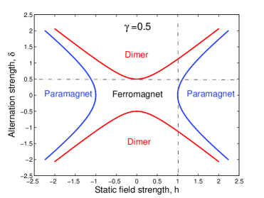
Figure 1: Phase diagram of the spin-$1/2$ XY alternating Hamiltonian given in Eq. (6) with $\gamma=0.5$.

In the general case, the boundaries between FM and PM phases, as well as between FM and DM phases, are characterized by second-order broken-symmetry QPTs. Interestingly, however, $E_{GS}$ develops weak singularities at

$$(h_{c},\delta_{c})=(0,\delta=\pm\gamma)\,,\hskip 28.45274pt(h_{c},\delta_{c})=(\pm 1,\delta=0)\,,$$ (8)

where fourth-order broken-symmetry QPTs occur along the paths approaching the QCPs (Fig. 1, dashed-dotted lines). In the isotropic limit ($\gamma=0$), an insulator-metal Lifshitz QPT occurs from a gapped to a gapless phase, with no broken-symmetry order parameter. For simplicity, we shall primarily focus on gapped quantum phases in what follows, thus $\gamma>0$. Standard finite-size scaling analysis reveals that new quantum critical behavior emerges in connection with the alternating fourth-order QCPs in Eq. (8)[15]. Thus, in addition to the usual Ising universality class, characterized by critical exponents $\nu=1,z=1$, an alternating universality class occurs, with critical exponents $\nu=2,z=1$.

The key step toward applying GE as a QPT indicator is to identify a (Lie) algebra of observables whose expectations reflect the changes in the GS as a function of the control parameters. It is immediate to realize that Hamiltonian Eq. (6), once written in fermionic language, is an element of the Lie algebra $\mathfrak{so}(2N)$, which includes arbitrary bilinear fermionic operators. As a result, the GS is always a GCS of $\mathfrak{so}(2N)$, and GE relative to $\mathfrak{so}(2N)$ carries no information about QCPs. However, the GS becomes a GCS of the number-conserving sub-algebra $\mathfrak{u}(N)$ in both the fully PM and DM limit. This motivates the choice of the fermionic $\mathfrak{u}(N)$-algebra discussed in Example 2 as a natural candidate for this class of systems. Taking advantage of the symmetries of this Hamiltonian, the fermionic purity given in Eq. (4) becomes:

$$P_{\mathfrak{u}(N)} = \frac{8}{N}\sum_{k\in K_{+}}\bigg{\{}\Big{[}|\langle a_{k}^{\dagger}b_{k}\rangle|^{2}+|\langle a_{-k}^{\dagger}b_{-k}\rangle|^{2}\Big{]}\hskip 113.81102pt$$

$$+ \frac{4}{N}\Big{[}\langle a_{k}^{\dagger}a_{k}-1/2\rangle^{2}+\langle a_{-k}^{\dagger}a_{-k}-1/2\rangle^{2}+\langle b_{k}^{\dagger}b_{k}-1/2\rangle^{2}+\langle b_{-k}^{\dagger}b_{-k}-1/2\rangle^{2}\Big{]}\bigg{\}}$$

Analytical results for $P_{\mathfrak{u}(N)}$ are only available for $\delta=0$, where GE sharply detects the PM-FM QPT in the XY model [10]. Remarkably, ground-state fermionic GE still faithfully portraits the full quantum phase diagram with alternation. First, derivatives of $P_{\mathfrak{u}(N)}$ develop singular behavior only at QCPs, see Fig. 2 (left). Furthermore, GE exhibits the correct scaling properties near QCPs [10]. By taking a Taylor expansion, $P_{\mathfrak{u}(N)}(h)-P_{\mathfrak{u}(N)}(h_{c})\sim{\xi}^{-1}\sim(h-h_{c})^{\nu}$, where $\xi$ is the correlation length, the static critical exponent $\nu$ may be extracted from a log-log plot of $P_{\mathfrak{u}(N)}$ for both the Ising and the alternating universality class, as demonstrated in Fig. 2 (right).

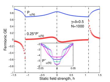
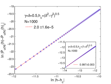
Figure 2: $P_{\mathfrak{u}(N)}$ as a static QPT indicator. Left panel: Purity and rescaled purity derivative vs magnetic field strength. Inset: second derivative for $N=1000,2000,4000,8000$ (top to bottom). Right panel: Determination of $\nu$ for both the alternating and Ising (inset) universality class.

3.2 Dynamic QPTs

While the above studies provide a satisfactory understanding of static quantum critical properties, dynamical aspects of QPTs present a wealth of additional challenges. To what extent can non-equilibrium properties be predicted by using equilibrium critical exponents? The simplest dynamical scenario one may envision arises when a single control parameter is slowly changed in time with constant speed $\tau_{q}>0$, that is, $g(t)-g_{c}={(t-t_{c})}/{\tau_{q}}$, so that a QCP is crossed at $t=t_{c}$ ($t_{c}=0$ without loss of generality). The typical time scale characterizing the response of the system is the relaxation time $\tau={\hbar}/{\Delta}\sim{|g(t)-g_{c}|^{-z\nu}}$, $\Delta$ being the gap between the ground state and first accessible excited state and $z$ the dynamic critical exponent [1]. Since the gap closes at QCPs in the thermodynamic limit, $\tau$ diverges even for an arbitrarily slow quench, resulting in a critical slowing-down. According to the so-called Kibble-Zurek mechanism (KZM) [18], a crossover between an (approximately) adiabatic regime to an (approximately) impulse regime occurs at a freeze-out time $-\hat{t}$, whereby the system’s instantaneous relaxation time matches the transition rate,

$$\tau(\hat{t})=|(g(\hat{t})-g_{c})/g^{\prime}(\hat{t})|\,,\;\;\;\;\;\hat{t}\sim\tau_{q}^{\nu z/(\nu z+1)}\,,$$

resulting in a predicted scaling of the final density of excitations as

$$n(t_{F})\sim\tau_{q}^{-\nu/(\nu z+1)}\,.$$ (10)

While agreement with the above prediction has been verified for different quantum systems [19], several key points remain to be addressed: What are the required physical ingredients for the KZM to hold? What features of the initial (final) quantum phase are relevant? How does dynamical scaling reflect into entanglement and other observable properties?

In our model, the time-evolved many-body state at instant time $t$, $|\Phi(t)\rangle=\prod_{k\in K^{+}}|\Phi_{k}(t)\rangle$, may still be expressed in the form of Eq. (7) for time-dependent coefficients $u_{k}^{(a)}(t)$, $a=1,\ldots,6$, computed from the solution of the Schrödinger equation, subject to the initial condition that $|\Phi(t\rightarrow-\infty)\rangle=|\Psi_{GS}(-\infty)\rangle$. The final excitation density is then obtained from the expectation value of the appropriate quasi-particle number operator over the final state,

$$n(t_{F})=\frac{1}{N}\langle\Phi(t_{F})|\sum_{k\in K_{+}}(\gamma_{k,3}^{\dagger}\gamma_{k,3}+\gamma_{k,4}^{\dagger}\gamma_{k,4})\,|\Phi(t_{F})\rangle\,.$$

As shown in Fig. 3 (left), the resulting value agrees with Eq. (10) over an appropriate $\tau_{q}$-range irrespective of the details of the QCP and the initial (final) quantum phase:

$$n(t_{F})^{Ising}\sim\tau_{q}^{-1/2}\,,\;\;\;\;\;n(t_{F})^{Alternating}\sim\tau_{q}^{-2/3}\,.$$

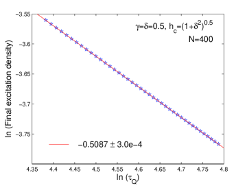
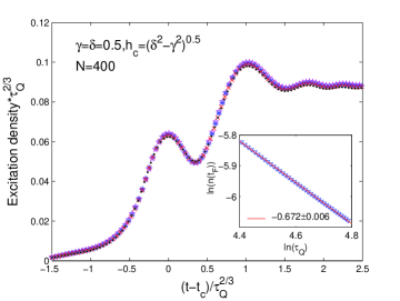
Figure 3: Dynamical scaling of the excitation density. Left panel: log-log plot for Ising universality class (FM to PM). Right panel: alternating universality class (FM to FM), with log-log scaling plot in the inset.

Remarkably, however, our results indicate that scaling behavior holds throughout the entire time evolution (see Fig. 3, right), implying the possibility to express the time-dependent excitation density as:

$$n(t)=\tau_{q}^{-\nu/(\nu z+1)}F\Big{(}\frac{t-t_{c}}{\hat{t}}\Big{)}\,,$$

where $F$ is a universal scaling function. Numerical results support the conjecture that similar universal dynamical scaling holds for arbitrary observables [17]. In particular, fermionic GE obeys scaling behavior across the entire dynamics provided that the amount relative to the instantaneous ground state $|\Psi(t)\rangle_{GS}$ is considered:

$$\Delta P_{\mathfrak{u}(N)}(t)\equiv P_{\mathfrak{u}(N)}(|\Phi(t)\rangle)-P_{\mathfrak{u}(N)}(|\Psi(t)\rangle_{GS})=\tau_{q}^{-\nu/(\nu z+1)}G\Big{(}\frac{t-t_{c}}{\hat{t}}\Big{)}\,,$$

for an appropriate scaling function $G$, see Fig. 4.

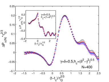
Figure 4: Dynamical scaling of $P_{\mathfrak{u}(N)}$ for the alternating and the Ising (inset) universality class.

It is important to stress that the above discussion applies to control paths which originate and end in gapped phases. In the isotropic limit $\gamma=0$, we observe no scaling of the form Eq. (10) if the system is driven to/from the superfluid gapless phase.

4 Conclusion

In addition to further demonstrating the usefulness of the GE notion toward characterizing static quantum critical phenomena, we have tackled the study of time-dependent QPTs in a simple yet illustrative scenario. Our analysis points to the emergence of suggestive physical behavior and a number of questions which deserve to be further explored. In particular, while for gapped systems as considered here, the origin of the observed universal dynamical scaling is likely to be rooted in the existence of a well-defined adiabatic (though non-analytic) limit – as independently investigated in Ref. Anatoli, a rigorous understanding remains to be developed. We expect that a GE-based perspective will continue to prove valuable to gain additional insight in quantum-critical physics.

References

- [1] S. Sachdev, Quantum Phase Transitions (Cambridge UP, Cambridge, 1999).
- [2] M. Greiner, O. Mandel, T. Esslinger, T. W. Hänsch, and I. Bloch, Nature 415, p. 39 (2002).
- [3] L. E. Sadler, J. M. Higbie, S. R. Leslie, M. Vengalattore, and D. M. Stamper-Kurn, Nature 443, p. 312 (2006).
- [4] P. Gegenwart et al., Phys. Rev. Lett., 89, p. 056402 (2002).
- [5] R. Jozsa and N. Linded, Proc. Roy. Soc. London A 459, p. 2001 (2003); G. Vidal, Phys. Rev. Lett. 91, p. 147902 (2003).
- [6] F. Verstraete and J. I. Cirac, arXiv: cond-mat/0407066 (2004); Phys. Rev. A 70, p. 060302(R) (2004).
- [7] D. Porras, F. Verstraete, and J. I. Cirac, Phys. Rev. B 73, p. 014410 (2006); G. Vidal, Phys. Rev. Lett. 93, p. 040502 (2004).
- [8] J. Eisert, Phys. Rev. Lett. 97, p. 260501 (2006); R. Somma, H. Barnum, G. Ortiz, and E. Knill, Phys. Rev. Lett. 97, p. 190501 (2006).
- [9] H. Barnum, E. Knill, G. Ortiz, and L. Viola, Phys. Rev. A, 68, p. 032308 (2003); H. Barnum, E. Knill, G. Ortiz, R. Somma, and L. Viola, Phys. Rev. Lett., 92, p. 107902 (2004).
- [10] R. Somma, G. Ortiz, H. Barnum, E. Knill, L. Viola, Phys. Rev. A 70, p. 042311 (2004); R. Somma, H. Barnum, E. Knill, G. Ortiz, and L. Viola, Int. J. Mod. Phys. B 20, 2760 (2006).
- [11] L. Amico, R. Fazio, A. Osterloh, and V. Vedral, arXiv: quant-ph/0703044 (2007).
- [12] L. Viola and H. Barnum, arXiv:quant-ph/0701124 (2007), and references therein.
- [13] M. Kindermann, Phys. Rev. Lett. 96, p. 240403 (2006).
- [14] P. Pfeuty, Ann. Phys. 57, p. 79 (1970); E. Barouch, B. M. McCoy, and M. Dresden, Phys. Rev. A 2, p. 1075 (1970).
- [15] O. Derzhko and T. Krokhmalskii, Czech. J. Phys. 55, p. 605 (2005); O. Derzhko, J. Richter, and T. Krokhmalskii, Phys. Rev. E 69, p. 066112 (2004).
- [16] K. Okamoto and K. Yasumura, J. Phys. Soc. Japan 59, p. 993 (1990).
- [17] S. Deng, G. Ortiz, and L. Viola, in preparation.
- [18] W. H. Zurek, U. Dorner, and P. Zoller, Phys. Rev. Lett. 95, p. 105701 (2005).
- [19] J. Dziarmaga, Phys. Rev. Lett. 95, p. 245701 (2005); F. M. Cucchietti, B. Damski, J. Dziarmaga, and W. H. Zurek, Phys. Rev. A 75, p. 023603 (2007).
- [20] A. Polkovnikov, Phys. Rev. B, 72, p. 161201 (2005); A. Polkovnikov and V. Gritsev, cond-mat/0706.0212 (2007).