Genetic selection of neutron star structure matching the X-ray observations

Abstract

Assuming a resonant origin of the quasiperiodic oscillations observed in the X-ray neutron star binary systems, we apply a genetic algorithm method for selection of neutron star models. It was suggested that pairs of kilo-hertz peaks in the X-ray Fourier power density spectra of some neutron stars reflect a non-linear resonance between two modes of accretion disk oscillations. We investigate this concept for a specific neutron star source. Each neutron star model is characterized by the equation of state (EOS), rotation frequency $\Omega$ and mass $M$. These determine the spacetime structure governing geodesic motion and position dependent radial and vertical epicyclic oscillations related to the stable circular geodesics. Particular kinds of resonances (KR) between the epicyclic frequencies, or the frequencies derived from them, can take place at special positions assigned ambiguously to the spacetime structure. The pairs of resonant eigenfrequencies relevant to those positions are therefore fully given by KR,$M,~{}\Omega$, EOS and can be compared to the observationally determined pairs of eigenfrequencies in order to eliminate the unsatisfactory sets (KR,$M,~{}\Omega$, EOS). For the elimination we use the advanced genetic algorithm. Genetic algorithm comes out from the method of natural selection when subjects with the best adaptation to assigned conditions have most chances to survive. The chosen genetic algorithm with sexual reproduction contains one chromosome with restricted lifetime, uniform crossing and genes of type 3/3/5. For encryption of physical description (KR,$M,~{}\Omega$, EOS) into chromosome we used Gray code. As a fitness function we use correspondence between the observed and calculated pairs of eigenfrequencies.

1 Introduction

Recently developed observational techniques provide good quality data from observations of quasiperiodic oscillations (QPOs) in black hole and neutron star sources [1]. It is shown that in the case of some neutron star atoll sources (e.g. 4U1636-53 [2]) the data can be well fitted by the so called multiresonant total precession model [1]. The fits give high precision values of the neutron star spacetime parameters; in addition, in some cases the rotation frequency of the neutron star is measured determined almost exactly from the QPO independent measurements. This enables us to put some limits on equations of state (EOS) describing the neutron star interior. Here we focus our attention of the EOS given by the Skyrmion interaction that are very well tuned to the data given by the nuclear physics [3]. Using the genetic algorithm method, which appears to be very fast and efficient, we select the acceptable EOS from 27 types of the Skyrmion EOS selected by other methods [3], concentrating on the source 4U 1636-53. For the other five atoll sources, the method gives similar results.

2 Fitting the QPO data

The results of recent studies of neutron star QPOs indicate that for a given source the upper and lower QPO frequency can be traced through the whole range of observed frequencies but the probability to detect both QPOs simultaneously increases when the frequency ratio is close to ratio of small natural numbers (namely 3/2, 4/3, 5/4 in the case of atoll sources studies recently, see [1]). Therefore, the multi–resonant orbital model based on the oscillation with Keplerian ($\nu_{\mathrm{K}}$) and epicyclic vertical ($\nu_{\theta}$) or radial ($\nu_{\mathrm{r}}$) frequencies was used to explain the observed data [1]. They are calculated assuming the spacetime given by the Hartle–Thorne metric [4, 5]. The fitting procedure have shown that the best results are obtained using the total precession model, where in all the sources the upper frequency $\nu_{\mathrm{u}}=\nu_{\mathrm{K}}$ and the lower frequency $\nu_{\mathrm{l}}=\nu_{\mathrm{T}}=\nu_{\mathrm{\theta}}-\nu_{\mathrm{r}}$ [1]. We concentrate here on the case of 4U 1636-53, when the mass and dimensionless spin of the neutron star are fitted to values ($\chi^{2}+1$ precision) in the range

$$M = 1.77\pm 0.07,~{}~{}~{}~{}j=0.051\pm 0.044,$$ (1)

$$M = 1.84\pm 0.07,~{}~{}~{}~{}j=0.101\pm 0.044.$$ (2)

This interval of allowed values of $M$ and $j$ will be used to test the EOS for the neutron star in the 4U 1636-53 source.

3 The neutron star structure

In neutron star, the strong gravity (i.e. Einsteins gravitational equations) must be relevant being crucial for the structure equations. The spacetime geometry is assumed to be stationary and axisymmetric, the perturbative approach of Hartle and Thorne [4] is used. One start with the spherically symmetric space time, given by Schwarzschild–like metric

$$\mathrm{d}s^{2} = -\mathrm{e}^{\nu}\mathrm{d}t^{2}+\left[1-2m(r)/r\right]^{-1}\mathrm{d}r^{2}$$ (3)

$$+ r^{2}\left(\mathrm{d}\theta^{2}+\sin^{2}\theta(\mathrm{d}\phi-\omega\mathrm{d}t^{2})\right].$$

To calculate structure of nonrotating, unperturbed star one has to integrate TOV equation

$$\frac{\mathrm{d}P}{\mathrm{d}r}=-\frac{Gm(r)\rho}{r^{2}}\frac{\left(1+P/\rho c^{2}\right)\left[1+4\pi r^{3}P/m(r)c^{2}\right]}{1-2Gm(r)/rc^{2}},$$ (4)

where

$$m(r)=\int\limits_{0}^{r}4\pi r^{2}\rho\mathrm{d}r$$ (5)

is the mass inside radius $r$. The integration is done outward from the center (for given values of central energy density $\rho_{\mathrm{c}}$) up to surface (where pressure vanishes). One obtains the global properties of non–rotating neutron star as its mass $M$, radius $R$ and the internal characteristic profiles as metric coefficients, pressure, energy density and number density of baryons expressed as functions of the radial coordinate distance from center.

The rotational effect is, in the linear approximation, given by the Hartle–Thorne metric [4].

$$\mathrm{d}s^{2} = -\mathrm{e}^{\nu}\left[1+2(h_{0}+h_{2}P_{2})\right]\mathrm{d}t^{2}$$ (6)

$$+ \frac{\left[1+2(m_{0}+m_{2}P_{2})/(r-2M)\right]}{1-2M/r}\mathrm{d}r^{2}$$

$$+ r^{2}\left[1+2(v_{2}-h_{2})P_{2}\right]$$

$$\times \left[\mathrm{d}\theta^{2}+\sin^{2}\theta(\mathrm{d}\phi-\omega\mathrm{d}t^{2})\right],$$

where $P_{2}=P_{2}(\cos\theta)=(3\cos^{2}\theta-1)/2$ is the Legendre polynomial of 2nd order $\omega$ is the angular velocity of local inertial frame, which is related to star’s angular velocity $\Omega$ and $h_{0},h_{2},m_{0},m_{2}$ are functions of $r$ and are all proportional to $\Omega^{2}$.The angular velocity $\omega$ can be found by solving equation

$$\frac{1}{r^{4}}\frac{\mathrm{d}}{\mathrm{d}r}\left(r^{4}j\frac{\mathrm{d}\tilde{\omega}}{\mathrm{d}r}\right)+\frac{4}{r}\frac{\mathrm{d}j}{\mathrm{d}r}\tilde{\omega}=0$$ (7)

where

$$j(r)=\mathrm{e}^{-\nu(r)/2}[1-2m(r)/r]^{1/2}.$$ (8)

One integrate equation (7) outward from center for arbitrarily chosen $\tilde{\omega}_{\mathrm{c}}$ with boundary condition $\mathrm{d}\omega/\mathrm{d}r=0$. At the surface one can calculate the angular momentum $J$ and frequency of rotation $\Omega$ corresponding to $\tilde{\omega}_{\mathrm{c}}$ from relations

$$J = \frac{1}{6}R^{4}\left(\frac{\mathrm{d}\tilde{\omega}}{\mathrm{d}r}\right)_{r=R}$$ (9)

$$\Omega_{\mathrm{new}} = \tilde{\omega}(R)+\frac{2J}{R^{3}}.$$ (10)

We take frequency of rotation $\Omega$ as an input parameter, thus after integration of eq. (7) we rescale the $\tilde{\omega}$ to obtain the right value of $\Omega$

$$\tilde{\omega}_{\mathrm{new}}(r)=\tilde{\omega}_{\mathrm{old}}(r)\frac{\Omega_{\mathrm{new}}}{\Omega_{\mathrm{old}}}.$$ (11)

After this one should calculate mass and pressure perturbation factors $m_{0}$ and $p_{0}$ from equations

$$\frac{\mathrm{d}m_{0}}{\mathrm{d}r} = 4\pi r^{2}\frac{\mathrm{d}E}{\mathrm{d}P}(E+P)p_{0}+\frac{1}{12}j^{2}r^{4}\left(\frac{\mathrm{d}\tilde{\omega}}{\mathrm{d}r}\right)^{2}$$ (12)

$$- \frac{1}{3}r^{3}\frac{\mathrm{d}j^{2}}{\mathrm{d}r}\tilde{\omega}^{2},$$

$$\frac{\mathrm{d}p_{0}}{\mathrm{d}r} = -\frac{m_{0}(1+8\pi r^{2}P)}{(r-2m)^{2}}-\frac{4\pi(E+P)r^{2}}{r-2m}p_{0}$$ (13)

$$+ \frac{1}{12}\frac{r^{4}j^{2}}{r-2m}\left(\frac{\mathrm{d}\tilde{\omega}}{\mathrm{d}r}\right)^{2}+\frac{1}{3}\frac{\mathrm{d}}{\mathrm{d}r}\left(\frac{r^{3}j^{2}\tilde{\omega}^{2}}{r-2m}\right).$$

The mass of rotational object is then given by

$$M(R)=M_{0}(R)+m_{0}(R)+J^{2}/R^{3}.$$ (14)

In the next approximation, the quadrupole moment $q$ of the star is introduced. The fitting procedure show that $q\sim j^{2}$ [1] where $j=J/M^{2}$. Therefore, the spacetime could be considered quasi-Kerr and the Kerr metric and related formula of the orbital motion could be used.

4 Skyrmion interactions and realated EOS

The effective Skyrmion interaction implies a variety of parametrization in the framework of mean–field theory. All give similar agreement with experimentally established nuclear ground states at the saturation density $n_{0}$, but they imply varying behaviour of both symmetric and asymmetric nuclear matter when density grows (up to $3n_{0}$).

The general form of effective Skyrme interaction implies total binding energy of a nuclei as the integral of an energy density functional $\mathcal{H}$, determined as a function of nine empirical parameters $t_{0},t_{1},t_{2},t_{3},x_{0},x_{1},x_{2},x_{3}$ and $\alpha$ in the form

$$\mathcal{H}=\mathcal{K}+\mathcal{H}_{0}+\mathcal{H}_{3}+\mathcal{H_{\mathrm{eff}}},$$ (15)

where the kinetic term $\mathcal{K}=\left(\hbar/2m\right)\tau$, is given by the kinetic densities $\tau=\tau_{\mathrm{n}}+\tau_{\mathrm{p}}$, with $\tau$ being the total density,$\tau_{\mathrm{n}}$ ($\tau_{\mathrm{p}}$)is the neutron (proton) density. The other terms are

given by the relations

$$\mathcal{H}_{0} = \frac{1}{4}t_{0}\left[(2+x_{0})n^{2}-(2x_{0}+1)(n_{p}^{2}+n_{n}^{2})\right]$$ (16)

$$\mathcal{H}_{3} = \frac{1}{24}t_{3}n^{\alpha}\left[(2+x_{3})n^{2}-(2x_{3}+1)(n_{p}^{2}+n_{n}^{2})\right]$$ (17)

$$\mathcal{H}_{eff} = {1}{8}\left[t_{1}(2+x_{1})+t_{2}(2+x_{2})\right]\tau_{n}$$ (18)

$$+ \frac{1}{8}\left[t_{2}(2x_{2}+1)-t_{1}(2x_{1}+1)\right](\tau_{p}n_{p}+\tau_{n}n_{n})$$

The pressure is then given by

$$P(n_{\mathrm{b}},I)=n^{2}_{\mathrm{b}}\frac{\partial\varepsilon}{\partial n_{\mathrm{b}}},$$ (19)

where $\varepsilon$ is the binding energy per particle and $I=(N-Z)/A$ denotes assymetry of nuclear matter.

In [3], 87 different Skyrme parametrization were limited to 27, using limits implied by the spherically symmetric models of neutron star models and by experimentally tested properties of nuclear matter. Here, we shall test acceptability of nine of these 27 Skyrme parametrization to the limits put by QPO measurements and using axisymmetric models in first approximations with respect to the star rotation.

5 Determination of neutron star structure using genetic algorithm

Genetic algorithm (GA) appears from method of natural selection, when subjects with best adaptation to assigned conditions have highest chance to survive [6]. GA takes into account the following natural mechanism - mutation and lifetime limit restricting risk of degradation, which is kept in local extreme from optimization viewpoint. GA has iteration character. GA doesn’t work with separate result in particular iterations, but with population. In each iteration GA works with several (generally a lot of results, standard value is hundreds) results, which are included in the population trying to ensure appearance of still better results via genetic operations with these results. Generally, the GA scheme is given in the form

$$GA=(N,P,f,\Theta,\Omega,\Psi,\tau)$$ (20)

where $P$ is population containing $N$ elements, $\Theta$ is parent selection operator which selects $u$ elements from $P$. Evaluation for each chromosome performed by the fitness function $f$.

$$f:S_{i}\leftarrow R,~{}i=1,...N.$$ (21)

Genetic operators included in $\Omega$ are namely crossover operator $\Omega_{\mathrm{C}}$, mutation operator $\Omega_{\mathrm{M}}$ and others problem-oriented or implementation-oriented specific operators, which all together generate $v$ offspring from $u$ parents. $\Psi$ is deletion operator, which removes $v$ selected elements from actual population $P(t)$. $v$ elements is add to new population $P(t+1)$ after it, $\tau$ is stop-criterion. Parent selection operator $\Theta$ and genetic operators $\Omega$ have stochastic character, deletion operator $\Psi$ is generally deterministic.

We have selected GA with sexual reproduction containing one chromosome with restricted lifetime parameter, 5 iterations. The crossover operator is selected with uniform crossing, using genes of type 3/3/5. We used the Gray code for encrypt parameters to chromosomes, which is useful by reason of bypassing so-called Hamming barrier.

Chromosomes are compound of genes; each gene presents 1 bit value. However, genes contain more than 1 bit (using the redundancy encrypt). Bit values inside a gene are mapped onto outside value of gene (0 or 1) via specific map function, in which border between 0 and 1 is not crisp, but there exists so-called “shade zone”, where value carried by the gene is determined randomly. [8, 9].We pressed number of members in each generation to 400 (see Fig.1) and interate 40 generations. We define two task of selection neutron star structure. The first one determines $\rho_{\mathrm{c}}$, $\Omega$ with preset EOS where fitness function f is $\chi^{2}$ [1]. It is important to say here, that at present the fitness function is tabled. The second one determines the EOS, $\rho_{\mathrm{c}}$, $\Omega$ with using fitness function $\chi^{2}$. Both tasks put limits on the EOS under consideration. Overcoming those limits implies removing the corresponding chromosomes by setting value of fitness function to a maximum value ($10^{200}$). For a given EOS allowed neutron star structure is provided the GA described above and fitness function $\chi^{2}$. The chromosome structure is given by two values, central density and rotation frequency. Interval of central density we choose from $0.4\cdot 10^{15}$ to $3.3\cdot 10^{15}~{}\mathrm{g.cm}^{-3}$.

In the first task, partition of central density is set to 4096 (12 bits). Interval of rotation frequency is set from 50 to 8000 and partition to 8192 (13 bits). Following table shows determination of central density (in units of $10^{15}~{}\mathrm{g.cm}^{-3}$) and rotation frequency for given number of EOS.

Table 1: Fitness function and corresponding parameters for all tested EOS, $\Omega\in(50;8000)$

EOS type	$\rho_{c}$	$\Omega$	Fitness
0-SkT5	2.1244	964.17	56.556
1-SkO’	1.5575	979.70	56.686
2-SkO	1.3987	711.85	56.601
3-SLy4	1.4896	1373.71	57.292
4-GS	1.1225	743.89	57.223
5-SkI2	1.1185	1241.72	57.688
6-SkI5	0.9359	791.43	57.059
7-SGI	1.0170	986.49	57.028
8-SV	0.7889	590.55	56.393

Because the resulting frequencies do not fit the observed rotation frequency interval [7], and also the fitness function has too many of local minima with same value for different combination of $\rho_{\mathrm{C}},~{}\Omega$ ,we make determination of values mentioned before, but we set range of rotation frequencies from 1827.21 to 1828.03 with partition 64 (6 bit).

Table 2: Fitness function and corresponding parameters for all tested EOS, $\Omega\in(1827.21;1828.03)$

EOS type	$\rho_{c}$	$\Omega$	Fitness
0-SkT5	2.9978	1827.928	62.979
1-SkO’	1.7896	1827.453	57.542
2-SkO	1.6762	1827.210	57.899
3-SLy4	1.5747	1827.300	57.611
4-GS	1.3084	1827.236	57.830
5-SkI2	1.2174	1827.505	58.061
6-SkI5	1.0803	1827.377	58.277
7-SGI	1.1146	1827.492	58.658
8-SV	0.8858	1827.428	58.45

Clearly, for selecting the most convenient EOS we need referenced $\chi^{2}$ value as global minimum $\chi^{2}$ over all EOS. Thus we make second task, determination of the best resulting neutron star structure over all used EOS. The corresponding EOS value is given by zero based EOS number (4 bits).

Table 3: Global minima for $\Omega\in(1827.21;1828.03)$

$\Omega_{\mathrm{min}}$	$\Omega_{\mathrm{max}}$	Fitness	EOS	$\rho_{c}$	$\Omega$
1827.21	1828.03	57.542	1	1.79021	1827.66

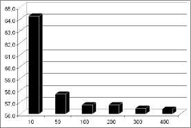
Figure 1: Dependency of $\chi^{2}$ on number of members in each generation

6 Conclusions

Analysis of QPO’s in neutron star atoll sources in the framework of Hartle–Thorne geometry gives a very detailed data (neutron star parameters as mass,spin and quadrupole momentum) that could be quite well used for constraining the wide scale of allowed EOS constraining the structure of neutron stars by solving the complex set of structure differential equations. The testing by standard approaches is a long time consuming procedure. Here, we show in the case of atoll source 4U 1636–53 that the genetic algorithm method could make the proper selection in a wide sample of EOS of Skyrmion type in a very efficient and short way (with same precision and the time consumed for the GA about 30 minutes, being by orders shorter that the time consumed by the standard methods). We can conclude that using the GA with chromosome (EOS,$\rho_{c}$, $\Omega$) and putting physically motivated restrictions on the angular velocity ($\Omega$) and central density ($\rho_{c}$) governing the neutron star model being an output of the structure equations and the fitness function $\chi^{2}$ in the algorithm procedure, we are able to find the most probably structure of neutron star that fits the observed QPO data, with respect to observed rotational frequency for the source 4U 1636–53. It is given by the chromosome ($1,~{}1.79\cdot 10^{15},~{}1837.66$).

We expect that the method allows much strongest test by the genetic algorithm including the quadrupole momentum calculated directly without using the quasi–Kerr approximation $q\sim j^{2}$.

7 Acknowledgement

This work was supported by Czech grants MSM 4781305903 (Z. S., P. C. and G. T.) and LC 06014 (M. U. and P. B.).

References

- [1] Z. Stuchlik, G. Török, P.Bakala “On a multi-resonant origin of high frequency quasiperiodic oscillations in the neutron-star X-ray binary 4U 1636-53”, http://arxiv.org/abs/0704.2318
- [2] D. Barret, J. -F. Olive, M. C. Miller “ Drop of coherence of the lower kilo-Hz QPO in neutron stars: Is there a link with the innermost stable circular orbit?” Astronomische Nachrichten , Vol.326, 2006, 9, p.808-811
- [3] J. Rikovska Stone, J. C. Miller, R. Koncewicz, P. D. Stevenson, M. R. Strayer “Nuclear matter and neutron-star properties calculated with the Skyrme interaction”, Physical Review C , Vol. 68, 2003, pp. 034324-1 – 034324-16
- [4] J. B. Hartle, K. Thorne “Slowly rotating relativistic stars II. Model for neutron stars and supermassive stars” The Astrophysical Journal , Vol. 153, 1968, pp. 807 –834
- [5] S. Chandrasekhar, J. C. Miller “On slowly rotating homogeneous masses in general relativity” MNRAS, Vol. 167, 1974, pp. 63-79
- [6] D. E. Goldberg Genetic Algorithms in Search, Optimization, and Machine Learning, Addison-Wesley Publ. Comp., INC., 1989
- [7] F. K. Lamb “High Frequency QPOs in Neutron Stars and Black Holes: Probing Dense Matter and Strong Gravitational Fields” http://arxiv.org/abs/0705.0030
- [8] P. Cermak “Parameters optimization of fuzzy–neural model using GA” Int. Journal of Computational Intelligence Theory and Practice Vol. 1., 2006, pp. 23 – 30
- [9] P. Cermak, P. Chmiel “Parameters optimization of fuzzy-neural dynamic models”, 23rd International Conference of the North American Fuzzy Information Processing Society June 27-30 , 2004 Banff, AB, Canada, pp. 762-767