Reflection and Refraction of Bose-condensate Excitations

Abstract

We investigate the transmission and reflection of Bose-condensate excitations in the low energy limit across a potential barrier separating two condensates with different densities. The Bogoliubov excitation in the low energy limit has the incident angle where the perfect transmission occurs. This condition corresponds to the Brewster’s law for the electromagnetic wave. The total internal reflection of the Bogoliubov excitation is found to occur at a large incident angle in the low energy limit. The anomalous tunneling named by Kagan et al. [Yu. Kagan et al., Phys. Rev. Lett., 90, 130402 (2003)] can be understood in terms of the impedance matching. In the case of the normal incidence, comparison with the results in Tomonaga-Luttinger liquids is made.

I Introduction

The transmission and the reflection are basic concepts in physics, that have been studied for strings, elastic bodies, fluids, electromagnetic waves, quantum particles, Tomonaga-Luttinger liquids and so on. The present paper is devoted to the study of the transmission and the reflection of collective excitations in the condensed Bose system. This proceeds from the earlier study of the so-called anomalous tunneling Kagan2003 , which is described as follows: Bogoliubov excitations transmit perfectly through the potential barrier separating two condensates in the low energy limit. This is in markedly contrast to single particle tunneling in the usual quantum mechanics, where the perfect reflection occurs in the low energy limit.

We review a rough sequence of studies of the anomalous tunneling. Kovrizhin initially discussed the transmission coefficient of Bogoliubov excitations through the $\delta$-function potential barrier Kovrizhin2001 . Kagan et al. also studied the tunneling of Bogoliubov excitations through the rectangular potential Kagan2003 . Through the study in Ref. Kagan2003 , Kagan et al. pointed out that this phenomenon is anomalous, in comparison to the usual quantum tunneling of a single particle.

Danshita et al. considered the transmission of Bogoliubov excitations across the $\delta$-function barrier separating two condensates with different macroscopic phases Danshita2006 . They found that the anomalous tunneling disappears when the phase difference reaches the critical value giving the maximum supercurrent of the condensate.

These works were done using the one-dimensional potential. On the other hand, the problem of Bogoliubov excitations scattered by a spherical potential was examined Padmore1972 ; FujitaMThesis ; FujitaUnpublished . The energy dependence of the cross section of the low energy scattering by the spherical potential is consistent with the Rayleigh scattering of a sound wave in the classical wave mechanics, i.e., the cross section vanishes in the low energy limit FujitaMThesis ; FujitaUnpublished .

Using the fact that the wave function of the excited state in the low energy limit corresponds to the macroscopic wave function of the condensate Fetter1972 , Kato et al. concluded that the anomalous tunneling occurs for a potential barrier $V(x)$ being arbitrary symmetric function ($V(-x)=V(x)$) Kato2007 . They also indicated that the perfect tunneling appears even at finite temperatures within the scheme of the Popov approximation Kato2007 .

In the Tomonaga-Luttinger liquids, on the other hand, the perfect transmission has been also discussed in the context of quantum wire, using the renormalization-group Kane1992 , and considering the multiple reflections Safi1995 . Especially, using the renormalization-group theory, it was shown that the barrier is an irrelevant perturbation in an attractive fermion system Kane1992 . That is to say, the perfect transmission is known to occur in Tomonaga-Luttinger liquids in superconducting phase.

As seen in the above, the property of the transmission of the Bogoliubov excitation in the low energy limit has not only a specific character of the condensed Bose system but also something in common with that of the classical wave mechanics and that of the Tomonaga-Luttinger liquids. From this point of view, we have three aims in this paper as follows: (i) exposing novel phenomena of the transmission and the reflection of the Bogoliubov phonon, (ii) giving a physical implication about the anomalous tunneling analogous to the classical wave mechanics, (iii) comparing the result of the tunneling problem of the Bogoliubov phonon with that of the Tomonaga-Luttinger liquids.

To achieve these aims, we investigate the tunneling problem of the Bogoliubov phonon through the arbitrary potential barrier separating two condensates with different densities. We consider that the incident Bogoliubov phonon does not only run toward the wall perpendicularly but also runs toward the wall with an arbitrary incident angle. This extended problem is analogous to the problem of the reflection and the refraction of a wave at the interface between two different mediums.

We may summarize the results of this paper as follows: (i) The Bogoliubov phonon has an incident angle where the perfect transmission occurs between condensates with different densities. This condition corresponds to the Brewster’s law, i.e., the sum of the incident angle and the refracted angle is equal to $\pi/2$. There also exists the total internal reflection of the Bogoliubov excitation in the low energy limit. (ii) The perfect transmission of the Bogoliubov excitation in the low energy limit can be regarded as a result of the impedance matching between equivalent condensates separated by the potential wall. The impedance is inversely proportional to the sound speed of the Bogoliubov phonon. (iii) At normal incidence, our result in the low energy limit is consistent with the result obtained by the theory of Tomonaga-Luttinger liquids Safi1995 , when one uses the Luttinger liquid parameter for the weakly interacting Bose gases. We note that the negative density reflection in the interacting condensed Bose system cannot be necessarily identified with the Andreev reflection.

The outline of this paper is as follows. In Section II, we shall give a formulation of the problem, and derive the transmission and reflection coefficients. To obtain these coefficients, we use properties that the wave function of the excited state in the low energy limit corresponds to the condensate wave function, and the constancy of the energy flux. In Section III, we shall discuss results in accordance with three aims. We also propose future problems on the experimental and theoretical sides. In Section IV, we summarize our results.

II Formulation and Results

In this section, we derive the transmission and reflection coefficients of the Bogoliubov excitation in the low energy limit. We use the mean-field theory, say, the Gross-Pitaevskii equation Gross1961 ; Pitaevskii1961 and the Bogoliubov equation Bogoliubov1947 . To discuss the property of the Bogoliubov excitation in the low energy limit, we use the fact that the wave function of the excited state in the low energy limit corresponds to the macroscopic wave function of the condensate Fetter1972 . To evaluate the transmission and reflection coefficients, we use the constancy of the energy flux.

The stationary Gross -Pitaevskii equation written in dimensionless form is given by

$$\hat{\mathcal{H}}\overline{\Psi}(\overline{{\bf r}})=0,$$ (1)

where

$$\hat{\mathcal{H}}\equiv-\frac{1}{2}\overline{\nabla}^{2}+\overline{V}(\overline{\bf r})-1+|\overline{\Psi}(\overline{{\bf r}})|^{2},$$ (2)

and the Bogoliubov equation also written in dimensionless form is given by

$$\left(\begin{array}[]{cc}\hat{h}^{\prime}&-{\overline{\Psi}(\overline{{\bf r}})}^{2}\\ {\overline{\Psi}^{*}(\overline{\bf r})}^{2}&-\hat{h}^{\prime}\end{array}\right)\left(\begin{array}[]{cc}{u}(\overline{\bf r},\overline{\varepsilon})\\ {v}(\overline{\bf r},\overline{\varepsilon})\end{array}\right)=\overline{\varepsilon}\left(\begin{array}[]{cc}{u}(\overline{\bf r};\overline{\varepsilon})\\ {v}(\overline{\bf r};\overline{\varepsilon})\end{array}\right),$$ (9)

where $\hat{h}^{\prime}\equiv\hat{\mathcal{H}}+|\overline{\Psi}(\overline{{\bf r}})|^{2}$. We have introduced the following notations $\overline{\bf r}\equiv{\bf r}/\xi$, $\overline{\nabla}\equiv\xi\nabla$ $\overline{\Psi}(\overline{{\bf r}})\equiv\sqrt{g/\mu}\Psi({\bf r})$, $\overline{V}(\overline{\bf r})\equiv V({\bf r})/\mu$, and $\overline{\varepsilon}\equiv\varepsilon/\mu\varepsilon$, where $g(>0)$ is the coupling constant of the two-body short-range interaction, $\mu$ is the chemical potential, and $\xi$ is the healing length defined by $\xi\equiv\hbar/\sqrt{m\mu}$ with $m$ being the mass. Henceforth, we omit the bar for simplicity. We take the potential $V({\bf r})$ to be a function of $x$ and allow $V(x)$ to be asymmetric $V(x)\neq V(-x)$. We consider $V(x)$ being superposition of short-range potential near $x=0$ and a potential step with asymptotic form:

$$V(x)\rightarrow\left\{\begin{array}[]{ll}V_{\rm L},&\qquad{\rm for}\quad x\ll-1\\ V_{\rm R},&\qquad{\rm for}\quad x\gg 1,\end{array}\right.$$ (12)

where both $V_{\rm L}$ and $V_{\rm R}$ are smaller than unity. The profile of $V(x)$ is shown in Fig. 1.

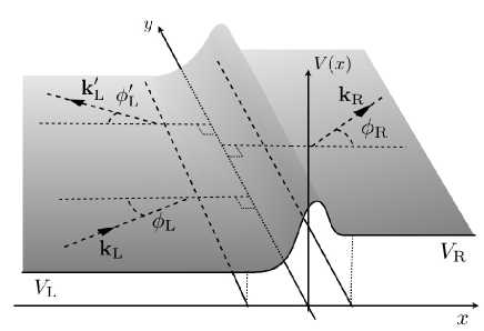
Figure 1: A schematic figure of the system. In this figure, we take $xy$ plane as an incident plane.

There are steady-states of a Bose-Einstein condensate even in the presence of a potential step Seaman2005 . In this paper, we shall treat a case without a supercurrent where the phase is spatially constant. Henceforth, $\Psi({\bf r})$ is considered to be real. In this situation, we have the following asymptotic behavior of the condensate wave function:

$$\Psi(x)\rightarrow\left\{\begin{array}[]{ll}\sqrt{1-{V}_{\rm L}},&\qquad{\rm for}\quad x\ll-1\\ \sqrt{1-{V}_{\rm R}},&\qquad{\rm for}\quad x\gg 1.\end{array}\right.$$ (15)

We note that our objective is to derive the transmission and reflection coefficients which can be adopted to the general case. However, we shall give an example here, in order to compare our general result with a concrete example. For instance, we assume that the potential $V(x)$ has the following behavior:

$$V(x)=\left\{\begin{array}[]{ll}0,&\qquad{\rm for}\quad x\leq 0,\\ V_{\rm b},&\qquad{\rm for}\quad 0<x\leq 1/\sqrt{2},\\ 0.8,&\qquad{\rm for}\quad 1/\sqrt{2}<x.\end{array}\right.$$ (19)

We use the strength of the potential barrier $V_{\rm b}$ as $V_{\rm b}=3$ and $5$. In Fig. 2, we show condensate wave functions obtained by numerical calculations, in the presence of the above potential $V(x)$. A solid line represents the numerical result for $V_{\rm b}=3$, and a dotted line represents the numerical result for $V_{\rm b}=5$. These numerical solutions satisfy the asymptotic behavior given in Eq. (15). When the potential energy in the asymptotic regime is less than the chemical potential, i.e., $V_{\nu}<\mu$ with $\nu={\rm L}$ for $x\ll-1$ and $\nu={\rm R}$ for $x\gg 1$, there are condensate wave functions spatially constant in the asymptotic regime, as shown in Fig. 2. Hence, Bogoliubov excitations even in the low energy limit exist in both sides of the potential barrier.

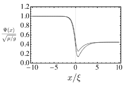
Figure 2: The numerical solutions of the condensate wave function. We use the potential energy as the function given in Eq. (19). A solid line represents the case for $V_{\rm b}=3$, and a dotted line represents the case for $V_{\rm b}=5$.

We shall consider the situation where a Bogoliubov excitation with a wavenumber vector ${\bf k}_{\rm L}$ runs against the potential wall at an angle $\phi_{\rm L}$ with respect to the normal vector of the wall (i.e., $x$-direction). The Bogoliubov phonon is split into a transmitted wave with a refraction having a wavenumber vector ${\bf k}_{\rm R}$ at an angle $\phi_{\rm R}$ and a reflected wave with ${\bf k}_{\rm L}^{\prime}$ at an angle $\phi_{\rm L}^{\prime}$ as shown in Fig. 1.

Owing to the translational invariance in $y$, $z$ directions, the Gross-Pitaevskii equation reduces to

$$\hat{h}\Psi(x)=0,$$ (20)

with

$$\hat{h}=-\frac{1}{2}\frac{d^{2}}{dx^{2}}+{V}(x)-1+\Psi^{2}(x).$$ (21)

The solution of the Bogoliubov equation has the form of

$$\left(\begin{array}[]{cc}{u}({\bf r};{\varepsilon})\\ {v}({\bf r};{\varepsilon})\end{array}\right)=\exp{(ik_{y}y+ik_{z}z)}\left(\begin{array}[]{cc}{u}(x;{\varepsilon})\\ {v}(x;{\varepsilon})\end{array}\right),$$ (26)

and the Bogoliubov equation is given by

$$\left(\begin{array}[]{cc}\hat{h}^{\prime\prime}&-\Psi^{2}(x)\\ \Psi^{2}(x)&-\hat{h}^{\prime\prime}\end{array}\right)\left(\begin{array}[]{cc}{u}(x;{\varepsilon})\\ {v}(x;{\varepsilon})\end{array}\right)=\varepsilon\left(\begin{array}[]{cc}{u}(x;{\varepsilon})\\ {v}(x;{\varepsilon})\end{array}\right),$$ (33)

where $\hat{h}^{\prime\prime}=\hat{h}+\Psi^{2}(x)+k_{\perp}^{2}/2$, and $k_{\perp}=\sqrt{k_{y}^{2}+k_{z}^{2}}$.

Let us consider asymptotic forms of a Bogoliubov mode. At $|x|\gg 1$ where $\Psi(x)\approx\sqrt{1-V_{\nu}}$ with $\nu={\rm L\,\,and\,\,R}$, the basis of the solution is given by two plane-wave solutions

$$\left(\begin{array}[]{cc}{u}(x;{\varepsilon})\\ {v}(x;{\varepsilon})\end{array}\right)=\exp{(\pm ik_{||,\nu}x)}\left(\begin{array}[]{cc}\tilde{u}_{\nu}(\varepsilon)\\ \tilde{v}_{\nu}(\varepsilon)\end{array}\right),$$ (38)

and exponentially growing or converging solutions

$$\left(\begin{array}[]{cc}{u}(x;{\varepsilon})\\ {v}(x;{\varepsilon})\end{array}\right)=\exp{(\pm\kappa_{\nu}x)}\left(\begin{array}[]{cc}\tilde{v}_{\nu}(\varepsilon)\\ -\tilde{u}_{\nu}(\varepsilon)\par\end{array}\right),$$ (43)

where

$$\tilde{u}_{\nu}(\varepsilon)\equiv\sqrt{\frac{\sqrt{(1-V_{\nu})^{2}+\varepsilon^{2}}}{2\varepsilon}+\frac{1}{2}},\qquad\quad\tilde{v}_{\nu}(\varepsilon)\equiv\sqrt{\frac{\sqrt{(1-V_{\nu})^{2}+\varepsilon^{2}}}{2\varepsilon}-\frac{1}{2}},$$ (44)

satisfying the normalization $|\tilde{u}_{\nu}(\varepsilon)|^{2}-|\tilde{v}_{\nu}(\varepsilon)|^{2}=1$. The wavenumber $k_{||,\nu}$ and the growing rate (or converging rate) $\kappa_{\nu}$ are given by, respectively,

$$\left\{\begin{array}[]{lll}k_{||,\nu}&=&\sqrt{k_{\nu}^{2}-k_{\perp}^{2}}\\ \kappa_{\nu}&=&\sqrt{2\left[1-V_{\nu}+\sqrt{\varepsilon^{2}+(1-V_{\nu})^{2}}\right]+k_{\perp}^{2}}\,\,,\end{array}\right.$$ (47)

where $k_{\nu}=\sqrt{2\left[\sqrt{(1-V_{\nu})^{2}+\varepsilon^{2}}-(1-V_{\nu})\right]}$.

Wavenumbers $k_{||,\nu}$ and $k_{\perp}$ which are, respectively, parallel and perpendicular components against the normal vector of the wall can be written as $k_{||,\nu}=k_{\nu}\cos{\phi_{\nu}}$ and $k_{\perp}=k_{\nu}\sin{\phi_{\nu}}$. Owing to the translational invariance in $y$, $z$ directions, we have the law of reflection

$$\phi_{\rm L}=\phi_{\rm L}^{\prime}.$$ (48)

Because of the law of reflection, there does not exist retroreflection in the weakly interacting condensed Bose system. That is to say, when the Bogoliubov excitation runs toward the wall with an incident angle, the reflected excitation does not go back the way one has come. We also have a relation between the incident angle and the transmitted angle given by

$$k_{{\rm L}}\sin{\phi_{{\rm L}}}=k_{{\rm R}}\sin{\phi_{{\rm R}}}.$$ (49)

In the low energy limit, the energy has the relation $\varepsilon\approx c_{\nu}k_{\nu}$, where $c_{\nu}$ is a sound speed of Bogoliubov phonon in the dimensionless form given by $c_{\nu}\equiv\sqrt{1-V_{\nu}}$. From the relation in Eq. (49), in the low energy limit, we recover the Snell’s law

$$\frac{\sin{\phi_{\rm L}}}{c_{\rm L}}=\frac{\sin{\phi_{\rm R}}}{c_{\rm R}}.$$ (50)

We assume that an incident wave comes from the left side of the potential barrier as shown in Fig. 1. Far from the barrier, exponentially-diverging components $e^{-\kappa_{\rm L}x}$ and $e^{\kappa_{\rm R}x}$ should be absent in the physical solution, and exponentially-converging components $e^{\kappa_{\rm L}x}$ and $e^{-\kappa_{\rm R}x}$ are negligible, so that we have the following asymptotic form:

$$\left(\begin{array}[]{cc}{u}(x;{\varepsilon})\\ {v}(x;{\varepsilon})\end{array}\right)=\left\{\begin{array}[]{ll}\left[a(\varepsilon)\exp{(ik_{||,{\rm L}}x)}+b(\varepsilon)\exp{(-ik_{||,{\rm L}}x)}\right]\left(\begin{array}[]{cc}\tilde{u}_{{\rm L}}(\varepsilon)\\ \tilde{v}_{{\rm L}}(\varepsilon)\end{array}\right),&{\rm for}\quad x\ll-1\\ \\ c(\varepsilon)\exp{(ik_{||,{\rm R}}x)}\left(\begin{array}[]{cc}\tilde{u}_{{\rm R}}(\varepsilon)\\ \tilde{v}_{{\rm R}}(\varepsilon)\end{array}\right),&{\rm for}\quad x\gg 1.\end{array}\right.$$ (60)

We introduce functions $S(x,\varepsilon)$ and $G(x,\varepsilon)$ Kato2007 ; FujitaMThesis ; Kagan2003 ; Kovrizhin2001 as

$$\left\{\begin{array}[]{ll}S(x;\varepsilon)\equiv u(x;\varepsilon)+v(x;\varepsilon)\\ G(x;\varepsilon)\equiv u(x;\varepsilon)-v(x;\varepsilon).\end{array}\right.$$ (63)

According to Eq. (60), we have the asymptotic form of the function $S(x;\varepsilon)$ in the low energy limit up to order ${\mathcal{O}}(\varepsilon^{1/2})$ as

$$\left\{\begin{array}[]{llllll}S(x;\varepsilon)&\sim&\varepsilon^{-1/2}\sqrt{2(1-V_{\rm L})}\left\{a(\varepsilon)+b(\varepsilon)+i\varepsilon\gamma_{\rm L}\left[a(\varepsilon)-b(\varepsilon)\right]x\right\},&&{\rm for}\quad x\ll-1\\ S(x;\varepsilon)&\sim&\varepsilon^{-1/2}\sqrt{2(1-V_{\rm R})}c(\varepsilon)\left(1+i\varepsilon\gamma_{\rm R}x\right),&&{\rm for}\quad x\gg 1,\end{array}\right.$$ (66)

where we define $\gamma_{\nu}\equiv\cos{\phi_{\nu}}/\sqrt{1-V_{\nu}}$.

From the Bogoliubov equation in Eq. (33), functions $S(x;\varepsilon)$ and $G(x;\varepsilon)$ satisfy following equations:

$$\left\{\begin{array}[]{ccc}\displaystyle{\left(\hat{h}+k_{\perp}^{2}/2\right)}S(x,\varepsilon)&=&\varepsilon G(x,\varepsilon)\\ \displaystyle{\left(\hat{h}^{(-)}+k_{\perp}^{2}/2\right)}G(x,\varepsilon)&=&\varepsilon S(x,\varepsilon),\end{array}\right.$$ (69)

where $\hat{h}^{(-)}=\hat{h}+2\Psi^{2}(x)$. We expand functions $S(x;\varepsilon)$ and $G(x;\varepsilon)$ with the energy $\varepsilon$ as

$$\left\{\begin{array}[]{ccc}S(x;\varepsilon)&=&\varepsilon^{-1/2}\sum\limits_{n=0}^{\infty}\varepsilon^{n}S^{(n)}(x)\\ G(x;\varepsilon)&=&\varepsilon^{-1/2}\sum\limits_{n=0}^{\infty}\varepsilon^{n}G^{(n)}(x).\end{array}\right.$$ (72)

We note that the factor $\varepsilon^{-1/2}$ comes from the normalization in Eq. (44). Equations for $S^{(0)}(x)$, $G^{(0)}(x)$, and $S^{(1)}(x)$ are given by

$$\left\{\begin{array}[]{ccc}\hat{h}S^{(0)}(x)&=&0\\ \hat{h}^{(-)}G^{(0)}(x)&=&0\\ \hat{h}S^{(1)}(x)&=&G^{(0)}(x).\end{array}\right.$$ (76)

First, we consider the solution $G^{(0)}$. The operator $\hat{h}^{(-)}$ has a second-order ordinary differential. The solution of $G^{(0)}$ can be written by

$$G^{(0)}(x) = B_{\rm I}g_{\rm I}(x)+B_{\rm II}g_{\rm II}(x),$$ (77)

with constants $B_{\rm I}$, $B_{\rm II}$ and two independent solutions $g_{\rm I}(x)$ and $g_{\rm II}(x)$ satisfying, respectively,

$$\left\{\begin{array}[]{ccc}\hat{h}^{(-)}g_{\rm I}(x)=0,\quad g_{\rm I}(x=0)=1,\quad\displaystyle{\left.\frac{dg_{\rm I}(x)}{dx}\right|_{x=0}=0}\\ \\ \hat{h}^{(-)}g_{\rm II}(x)=0,\quad g_{\rm II}(x=0)=0,\quad\displaystyle{\left.\frac{dg_{\rm II}(x)}{dx}\right|_{x=0}=1.}\end{array}\right.$$ (81)

At $|x|\gg 1$, the asymptotic behavior of $\hat{h}^{(-)}$ can be written as $-\frac{d^{2}}{2dx^{2}}+2(1-V_{\nu})$. Hence, any linear combination of $g_{\rm I}(x)$ and $g_{\rm II}(x)$ generally diverges exponentially at $|x|\gg 1$. On the other hand, $G^{(0)}$ should not have any exponentially diverging terms at $|x|\gg 1$. Thus, it is allowed that we set $B_{\rm I}=B_{\rm II}=0$ as in Ref. Kato2007 , and hence we do not have to treat the special solution of the inhomogeneous equation of the third equation in Eq. (76).

We shall consider general solutions of homogeneous equations given by

$$\hat{h}S^{(0)}(x)=0,\qquad\hat{h}S^{(1)}(x)=0.$$ (82)

Equations in Eq. (82) are second-order linear differential equations, and hence solutions $S^{(0)}(x)$ and $S^{(1)}(x)$ can be written as

$$\left\{\begin{array}[]{ccc}S^{(0)}=A_{\rm I}^{(0)}s_{\rm I}(x)+A_{\rm II}^{(0)}s_{\rm II}(x)\\ S^{(1)}=A_{\rm I}^{(1)}s_{\rm I}(x)+A_{\rm II}^{(1)}s_{\rm II}(x),\end{array}\right.$$ (85)

by using two independent solutions $s_{\rm I}(x)$ and $s_{\rm II}(x)$ satisfying

$$\left\{\begin{array}[]{ccc}\displaystyle{\hat{h}s_{\rm I}(x)=0,\quad s_{\rm I}(x=0)=1,\quad\left.\frac{ds_{\rm I}(x)}{dx}\right|_{x=0}=0}\\ \\ \displaystyle{\hat{h}s_{\rm II}(x)=0,\quad s_{\rm II}(x=0)=0,\quad\left.\frac{ds_{\rm II}(x)}{dx}\right|_{x=0}=1.}\end{array}\right.$$ (89)

At $|x|\gg 1$, the asymptotic behavior of $\hat{h}$ is described as $\hat{h}\sim-\frac{1}{2}\frac{d^{2}}{dx^{2}}$, so that we have solutions as

$$\left\{\begin{array}[]{ccc}s_{\rm I}(x)&\sim&\alpha_{{\rm I},\nu}+\beta_{{\rm I},\nu}x\\ s_{\rm II}(x)&\sim&\alpha_{{\rm II},\nu}+\beta_{{\rm II},\nu}x,\end{array}\right.$$ (92)

with $\nu={\rm L}$ for $x\ll-1$ and $\nu={\rm R}$ for $x\gg 1$.

As a result, we have the asymptotic behavior of the solution $S(x;\varepsilon)$ given by

$$S(x;\varepsilon) \sim \varepsilon^{-1/2}\left[A_{\rm I}(\varepsilon)\alpha_{{\rm I},\nu}+A_{\rm II}(\varepsilon)\alpha_{{\rm II},\nu}\right]$$ (93)

$$+\varepsilon^{-1/2}[A_{\rm I}(\varepsilon)\beta_{{\rm I},\nu}+A_{\rm II}(\varepsilon)\beta_{{\rm II},\nu}]x+{\mathcal{O}}(\varepsilon^{3/2}),$$

with $\nu={\rm L}$ and ${\rm R}$, where we define $A_{\rm I}(\varepsilon)\equiv A_{\rm I}^{(0)}+\varepsilon A_{\rm I}^{(1)}$ and $A_{\rm II}(\varepsilon)\equiv A_{\rm II}^{(0)}+\varepsilon A_{\rm II}^{(1)}$ and use Eq. (92).

Let us use the property that the wave function of the excited state in the low energy limit corresponds to the macroscopic wave function of the condensate Fetter1972 . Considering solutions $s_{\rm I,II}(x)$ satisfying $\hat{h}s_{\rm I,II}(x)=0$, the solution of the Gross-Pitaevskii equation $\hat{h}\Psi(x)=0$ can be written as

$$\Psi(x)=\Psi_{0}s_{\rm I}(x)+\Psi_{0}^{\prime}s_{\rm II}(x),$$ (94)

where $\Psi_{0}\equiv\Psi(x=0)$ and $\Psi_{0}^{\prime}\equiv\left.\frac{d\Psi(x)}{dx}\right|_{x=0}$. Using asymptotic forms for $s_{\rm I}(x)$ and $s_{\rm II}(x)$ in Eq. (92), we evaluate asymptotic behaviors of the condensate wave function as

$$\Psi(x)\sim(\Psi_{0}\alpha_{{\rm I},\nu}+\Psi_{0}^{\prime}\alpha_{{\rm II},\nu})+(\Psi_{0}\beta_{{\rm I},\nu}+\Psi_{0}^{\prime}\beta_{{\rm II},\nu})x,$$ (95)

with $\nu={\rm L}$ and ${\rm R}$.

We know that asymptotic behaviors of the condensate wave function are given in Eq. (15), so that we have constraints for coefficients $\alpha_{\rm I,\nu}$, $\alpha_{\rm II,\nu}$, $\beta_{\rm I,\nu}$, and $\beta_{\rm II,\nu}$ given by

$$\left\{\begin{array}[]{lll}\Psi_{0}\alpha_{{\rm I},\nu}+\Psi_{0}^{\prime}\alpha_{{\rm II},\nu}&=&\sqrt{1-V_{\nu}}\\ \Psi_{0}\beta_{{\rm I},\nu}+\Psi_{0}^{\prime}\beta_{{\rm II},\nu}&=&0,\end{array}\right.$$ (98)

where $\nu={\rm L}$ and ${\rm R}$. The second equation of Eq. (98) shows that vectors ${}^{\rm t}(\beta_{{\rm I},\nu},\beta_{{\rm II},\nu})$ and ${}^{\rm t}(\Psi_{0},\Psi_{0}^{\prime})$ are orthogonal. Thus, we write the vector ${}^{\rm t}(\beta_{{\rm I},\nu},\beta_{{\rm II},\nu})$ as

$$\left(\begin{array}[]{lll}\beta_{{\rm I},\nu}\\ \beta_{{\rm II},\nu}\end{array}\right)\equiv\tilde{\beta}_{\nu}\left(\begin{array}[]{c}\Psi_{0}^{\prime}\\ -\Psi_{0}\end{array}\right),$$ (103)

with a constant $\tilde{\beta}_{\nu}$.

Comparing Eq. (66) and Eq. (93), we have equations for coefficients ${A}_{\rm I,II}(\varepsilon)$, the amplitude transmission coefficient $t(\varepsilon)\equiv c(\varepsilon)/a(\varepsilon)$, and the amplitude reflection coefficient $r(\varepsilon)\equiv b(\varepsilon)/a(\varepsilon)$,

$$\left\{\begin{array}[]{llllll}{A}_{\rm I}(\varepsilon)\alpha_{\rm I,L}+{A}_{\rm II}(\varepsilon)\alpha_{\rm II,L}&=&\sqrt{2(1-V_{\rm L})}a(\varepsilon)[1+r(\varepsilon)]+{\mathcal{O}}(\varepsilon^{2})\\ {A}_{\rm I}(\varepsilon)\beta_{\rm I,L}+{A}_{\rm II}(\varepsilon)\beta_{\rm II,L}&=&i\sqrt{2}a(\varepsilon)[1-r(\varepsilon)]\varepsilon\cos{\phi_{\rm L}}+{\mathcal{O}}(\varepsilon^{2}),\end{array}\right.$$ (106)

and

$$\left\{\begin{array}[]{llllll}{A}_{\rm I}(\varepsilon)\alpha_{\rm I,R}+{A}_{\rm II}(\varepsilon)\alpha_{\rm II,R}&=&\sqrt{2(1-V_{\rm R})}a(\varepsilon)t(\varepsilon)+{\mathcal{O}}(\varepsilon^{2})\\ {A}_{\rm I}(\varepsilon)\beta_{\rm I,R}+{A}_{\rm II}(\varepsilon)\beta_{\rm II,R}&=&i\sqrt{2}a(\varepsilon)t(\varepsilon)\varepsilon\cos{\phi_{\rm R}}+{\mathcal{O}}(\varepsilon^{2}).\end{array}\right.$$ (109)

Using Eqs. (98), (103), (106), and (109), we have the amplitude transmission coefficient $t(\varepsilon)$ and the amplitude reflection coefficient $r(\varepsilon)$ in the low energy limit $\varepsilon\rightarrow 0$

$$\left\{\begin{array}[]{lll}\lim\limits_{\varepsilon\rightarrow 0}t(\varepsilon)&=&\displaystyle{\frac{2\zeta_{\rm R}}{\zeta_{\rm R}+\zeta_{\rm L}}}\\ \\ \lim\limits_{\varepsilon\rightarrow 0}r(\varepsilon)&=&\displaystyle{\frac{\zeta_{\rm R}-\zeta_{\rm L}}{\zeta_{\rm R}+\zeta_{\rm L}}},\end{array}\right.$$ (113)

where we define $\zeta_{\nu}\equiv\tilde{\beta}_{\nu}/\cos{\phi_{\nu}}$.

We shall consider the relation between $\zeta_{\rm L}$ and $\zeta_{\rm R}$ on the basis of constancy of energy flux. According to Ref. Kagan2003 , one has the energy flux averaged over the time in dimensionless form given by

$$\langle{\bf Q}({\bf r})\rangle = \frac{\varepsilon}{2}{\rm Im}\left[S^{*}({\bf r})\nabla S({\bf r})+G^{*}({\bf r})\nabla G({\bf r})\right].$$ (114)

We shall consider the asymptotic behavior of the energy flux parallel to the normal vector of the wall by using Eq. (60). The asymptotic behavior of the energy flux in the $x$-direction for $x\ll-1$ is given by

$$\langle Q_{||,{\rm L}}\rangle\sim{\varepsilon}\left(|\tilde{u}_{+,{\rm L}}|^{2}+|\tilde{v}_{+,{\rm L}}|^{2}\right)k_{||,{\rm L}}\left[1-|r(\varepsilon)|^{2}\right]|a(\varepsilon)|^{2}.$$ (115)

On the other hand, we have the asymptotic form of the energy flux in the $x$-direction for $x\gg 1$ given by

$$\langle Q_{||,{\rm R}}\rangle\sim{\varepsilon}\left(|\tilde{u}_{+,{\rm R}}|^{2}+|\tilde{v}_{+,{\rm R}}|^{2}\right)k_{||,{\rm R}}|t(\varepsilon)|^{2}|a(\varepsilon)|^{2}.$$ (116)

In the low energy limit, the energy flux can be written as

$$\left\{\begin{array}[]{lll}\langle Q_{||,{\rm L}}\rangle&\sim&\varepsilon c_{\rm L}\cos{\phi_{\rm L}}\left[1-|r(\varepsilon)|^{2}\right]|a(\varepsilon)|^{2}\\ \langle Q_{||,{\rm R}}\rangle&\sim&\varepsilon c_{\rm R}\cos{\phi_{\rm R}}|t(\varepsilon)|^{2}|a(\varepsilon)|^{2}.\end{array}\right.$$ (119)

Regarding the constancy of the energy flux $\langle Q_{||,{\rm L}}\rangle=\langle Q_{||,{\rm R}}\rangle$ as the constraint for the variables $\zeta_{\rm L}$ and $\zeta_{\rm R}$, we obtain the ratio

$$\frac{\zeta_{\rm L}}{\zeta_{\rm R}}=\frac{c_{\rm R}}{c_{\rm L}}\frac{\cos{\phi_{\rm R}}}{\cos{\phi_{\rm L}}}.$$ (120)

As a result, we have the amplitude transmission coefficient $t(\varepsilon)$ and the amplitude reflection coefficient $r(\varepsilon)$ in the low energy limit as

$$\lim\limits_{\varepsilon\rightarrow 0}t(\varepsilon)=\frac{2c_{\rm L}\cos{\phi_{\rm L}}}{c_{\rm L}\cos{\phi_{\rm L}}+c_{\rm R}\cos{\phi_{\rm R}}},\qquad\qquad\lim\limits_{\varepsilon\rightarrow 0}r(\varepsilon)=\frac{c_{\rm L}\cos{\phi_{\rm L}}-c_{\rm R}\cos{\phi_{\rm R}}}{c_{\rm L}\cos{\phi_{\rm L}}+c_{\rm R}\cos{\phi_{\rm R}}}.$$ (121)

These amplitude transmission coefficient $t$ and amplitude reflection coefficient $r$ satisfy the relation: $1+r=t$, as seen in the classical wave mechanics. The transmission coefficient $T(\varepsilon)$ and the reflection coefficient $R(\varepsilon)$ are, respectively, given by ratios of the transmitted energy flux and of the reflected energy flux to the incident energy flux. In the low energy limit, $T(\varepsilon)$ and $R(\varepsilon)$ are, respectively, given by

$$\begin{array}[]{llllll}\lim\limits_{\varepsilon\rightarrow 0}T(\varepsilon)&=&\displaystyle\frac{4c_{\rm L}c_{\rm R}\cos{\phi_{\rm L}}\cos{\phi_{\rm R}}}{(c_{\rm L}\cos{\phi_{\rm L}}+c_{\rm R}\cos{\phi_{\rm R}})^{2}}\\ \\ \lim\limits_{\varepsilon\rightarrow 0}R(\varepsilon)&=&\displaystyle\frac{(c_{\rm L}\cos{\phi_{\rm L}}-c_{\rm R}\cos{\phi_{\rm R}})^{2}}{(c_{\rm L}\cos{\phi_{\rm L}}+c_{\rm R}\cos{\phi_{\rm R}})^{2}},\end{array}$$ (125)

satisfying the relation: $T(\varepsilon)+R(\varepsilon)=1$.

Equation (125) and the Snell’s law in Eq. (50) describe the transmission and the reflection of the Bogoliubov excitation in the low energy limit. We note that $T(\varepsilon\rightarrow 0)$ and $R(\varepsilon\rightarrow 0)$ in Eq. (125) do not depend on the detail of $V(x)$ near $x=0$; they depend on $V(x)$ only through the asymptotic values $V_{\rm L}$ and $V_{\rm R}$. The perfect transmission $T(\varepsilon\rightarrow 0)=1$ and $R(\varepsilon\rightarrow 0)=0$ follows from $c_{\rm L}=c_{\rm R}$, or equivalently $V_{\rm L}=V_{\rm R}$. This result is consistent with earlier studies Kagan2003 ; Danshita2006 ; Kato2007 ; Kovrizhin2001 . The transmission and reflection coefficients in Eq. (125) are similar to but different from those of the classical sound mechanics, as discussed later.

The formulation and the result up to the present is adopted to the existence of the potential $V(x)$ having the general form. Here, let us compare the transmission coefficient of our result with that obtained by the numerical calculation in the presence of a potential $V(x)$. We shall adopt the potential energy $V(x)$ given in Eq. (19). In Fig. 3, we show transmission coefficients $T$ in the low energy limit given in Eq. (125) and obtained by numerical calculations as a function of the energy $\varepsilon$. We set the incident angle as $\phi_{\rm L}=0$. Solid and dotted lines in Fig. 3 are numerical results in the case for $V_{\rm b}=3$ and $5$, respectively. The dot is our analytical result in the low energy limit. We note that the transmission coefficient obtained by numerical calculations reaches our analytical prediction as the incident energy goes to zero as seen in Fig. 3. This result means that the transmission and reflection coefficients in the low energy limit are independent of the potential barrier. These coefficients depend only on asymptotic values of the potential energy.

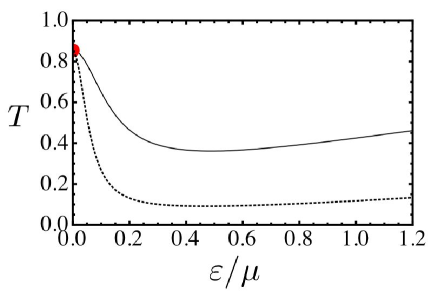
Figure 3: (Color online) The transmission coefficient $T$ as a function of the energy $\varepsilon$, where the incident angle $\phi_{\rm L}=0$. In the numerical calculation, we assume the potential energy given in Eq. (19). The solid and dotted lines in Fig. 3 are the numerical result in the case for $V_{\rm b}=3$ and $5$. The dot is our analytical prediction in the low energy limit.

III Discussion

In this section, we shall discuss the property of transmission and reflection of the Bogoliubov phonon. First, we shall show the phenomena of the Bogoliubov phonon having something in common with the electromagnetic wave. These are existences of the Brewster’s angle and the total internal reflection. Second, we shall give an interpretation of the anomalous tunneling in terms of the impedance matching. Third, we show the relation between the weakly interacting three-dimensional Bose gas and the one-dimensional Bose gas treated as the Tomonaga-Luttinger liquids. We also discuss the Andreev-like reflection, critically. Finally, we shall propose future problems on the experimental and theoretical sides.

III.1 Brewster’s Angle and Total Internal Reflection

In addition to the “ordinary” anomalous tunneling discussed in Refs. Kagan2003 ; Danshita2006 ; Kato2007 ; Kovrizhin2001 , we find another condition where we do have the perfect transmission of the Bogoliubov excitation in the low energy limit. When the incident Bogoliubov phonon has the incident angle $\phi_{\rm L,B}$ defined by

$$\tan{\phi_{\rm L,B}}\equiv{c_{\rm L}}/{c_{\rm R}},$$ (126)

we obtain the perfect transmission: $T=1$ and $R=0$. This incident angle $\phi_{\rm L,B}$ corresponds to the Brewster’s angle for the electromagnetic wave, satisfying the relation $\phi_{\rm L,B}+\phi_{\rm R}=\pi/2$ LandauElectromagnetic .

The transmission coefficient $T$ in the low energy limit as a function of the incident angle $\phi_{\rm L}$ is shown in Fig. 4. We use $V_{\rm L}=0$ and $V_{\rm R}=0.8$ as in Eq. (19). The incident angle where the perfect transmission occurs is seen in Fig. 4, as discussed above.

Figure 4: The transmission coefficient in the low energy limit as a function of the incident angle. We assume $V_{\rm L}=0$ and $V_{\rm R}=0.8$, consistent with the potential energy given in Eq. (19).

Moreover, we also find that the Bogoliubov excitation experiences the total internal reflection when the incident angle satisfies the condition $\phi_{\rm L}\geq\phi_{\rm L,c}$, where the critical angle $\phi_{\rm L,c}$ is defined by

$$\sin{\phi_{\rm L,c}}\equiv{c_{\rm L}}/{c_{\rm R}},$$ (127)

where $c_{\rm L}<c_{\rm R}$, i.e., $V_{\rm L}>V_{\rm R}$.

In Fig. 5, the transmission coefficient $T$ in the low energy limit in Eq. (125) is plotted in the $V_{\rm R}$ - $\phi_{\rm L}$ plane. We assume $V_{\rm L}=0$. The solid line at $V_{\rm R}=0$ represents the line where the “ordinary” anomalous tunneling occurs, i.e., the perfect transmission occurs independently of the incident angle $\phi_{\rm L}$. On the other hand, the dotted line represents the line where the perfect transmission occurs in the same condition as the Brewster’s law. As discussed above, there is a region where the total internal reflection occurs at $V_{\rm R}<V_{\rm L}=0$, as seen in Fig. 5.

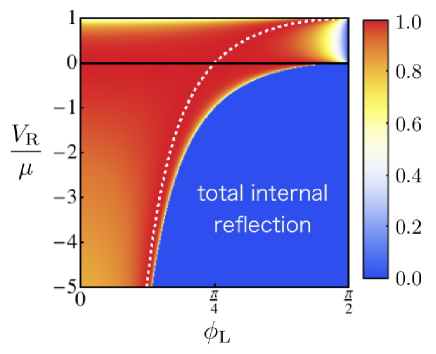
Figure 5: (Color online) The transmission coefficient in the low energy limit given by our analytical result is plotted in the $V_{\rm R}$ - $\phi_{\rm L}$ plane. We assume $V_{\rm L}=0$. The solid line at $V_{\rm R}=0$ represents the line where the “ordinary” anomalous tunneling occurs. The dotted line represents the line where the perfect transmission occurs in the same condition as the Brewster’s law. There is a region where the total internal reflection occurs.

III.2 Impedance Matching of Bogoliubov Phonon

The Brewster’s law and the total internal reflection of Bogoliubov excitations are naturally understood by recalling that expressions in Eq. (125) for the transmission and reflection coefficients have the same forms as those of the electromagnetic wave LandauElectromagnetic . The transmission and reflection coefficients of an electromagnetic wave going from the medium $\rm L$ to $\rm R$ are given by

$$\begin{array}[]{llllll}T&=&\displaystyle\frac{4Z_{\rm L}Z_{\rm R}\cos{\phi_{\rm L}}\cos{\phi_{\rm R}}}{(Z_{\rm R}\cos{\phi_{\rm L}}+Z_{\rm L}\cos{\phi_{\rm R}})^{2}}\\ \\ R&=&\displaystyle\frac{(Z_{\rm R}\cos{\phi_{\rm L}}-Z_{\rm L}\cos{\phi_{\rm R}})^{2}}{(Z_{\rm R}\cos{\phi_{\rm L}}+Z_{\rm L}\cos{\phi_{\rm R}})^{2}},\end{array}$$ (131)

when the electric field of the incident electromagnetic wave is perpendicular to the incident plane. The symbols $Z_{\rm L}$ and $Z_{\rm R}$ denote the impedance of the electromagnetic wave $Z^{\rm el}=\sqrt{\epsilon^{\prime}/\mu^{\prime}}$ for each medium. Here $\epsilon^{\prime}$ is the permittivity, and $\mu^{\prime}$ is the magnetic permeability. When the magnetic permeability for two mediums are equal, $Z_{\rm R}/Z_{\rm L}$ becomes equal to $c_{\rm L}/c_{\rm R}$, where $c_{\rm L}$ and $c_{\rm R}$ are light speeds in left and right mediums. As a result, Eq. (131) coincides with Eq. (125). We note that the anomalous tunneling discussed in Refs. Kagan2003 ; Danshita2006 ; Kato2007 ; Kovrizhin2001 can be then simply regarded as an impedance matching between two identical condensates, where the impedance of the Bogoliubov phonon is inversely proportional to the speed of Bogoliubov phonon.

It is worth mentioning that results in Eq. (125) are different from the transmission and reflection coefficients of the classical sound wave at the interface between two mediums; at the interface, the transmission and reflection coefficients

$$\begin{array}[]{llllll}T&=&\displaystyle\frac{4Z^{\rm ac}_{\rm L}Z^{\rm ac}_{\rm R}\cos{\phi_{\rm L}}\cos{\phi_{\rm R}}}{(Z^{\rm ac}_{\rm R}\cos{\phi_{\rm L}}+Z^{\rm ac}_{\rm L}\cos{\phi_{\rm R}})^{2}}\\ \\ R&=&\displaystyle\frac{(Z^{\rm ac}_{\rm R}\cos{\phi_{\rm L}}-Z^{\rm ac}_{\rm L}\cos{\phi_{\rm R}})^{2}}{(Z^{\rm ac}_{\rm R}\cos{\phi_{\rm L}}+Z^{\rm ac}_{\rm L}\cos{\phi_{\rm R}})^{2}}\end{array}$$ (135)

of the classical sound are given by the same form as Eq. (131). Here, $Z^{\rm ac}_{\rm L}$ and $Z^{\rm ac}_{\rm R}$ are the specific acoustic impedance $Z^{\rm ac}$ for each medium. $Z^{\rm ac}$ is defined as the ratio of the sound pressure to the particle velocity field and is given by $Z^{\rm ac}=\rho c$ with a mass density $\rho$ and a sound velocity $c$. The specific acoustic impedance for Bogoliubov excitations are given similarly from the calculation up to first order with respect to $u$ and $v$. The resultant specific acoustic impedance for Bogoliubov excitations is given by the product of the mass density of the condensate $(\propto 1-V_{\nu})$ and the sound speed $(\propto|1-V_{\nu}|^{1/2})$ for each condensate $\nu=$L and R. Considering $c_{\nu}\propto|1-V_{\nu}|^{1/2}$ in Eq. (125), it is obvious that Eqs. (125) and (135) are different.

The difference of the impedance between the classical sound and the Bogoliubov phonon comes from the difference of the boundary condition; in the classical sound wave, which is the first sound, say, the hydrodynamic collective mode, the transmission coefficient is derived from continuous conditions at the interface for the velocity perpendicular to the interface and for the pressure LandauFluid . On the other hand, in the Bogoliubov phonon, which is the zeroth sound, say, the collisionless collective mode 1990NozieresPines ; 1993Griffin ; 2000Giorgini , our result is derived from the constancy of the energy flux, and the property that the wave function of the Bogoliubov excitation in the low energy limit coincides with the macroscopic wave function of the condensate.

III.3 Comparison with Results on Tomonaga-Luttinger Liquids

We shall discuss the relation between transmission and reflection coefficients obtained in our system and those obtained in one-dimensional boson systems. As mentioned in the introduction, the perfect transmission in the Tomonaga-Luttinger liquids was investigated extensively and intensively in the study of quantum wire. Using the renormalization-group, Kane and Fisher showed that the barrier is an irrelevant perturbation, say, the perfect transmission occurs, when the Luttinger liquid parameter $K$ satisfies $K>1$ Kane1992 . In the fermion case, $K>1$ corresponds to an attractive fermion system, $K=1$ a free fermion system, and $1>K>0$ a repulsive fermion system Giamarchi . Safi and Schulz investigated the transport through a one-dimensional wire of interacting electrons connected to leads sufficiently longer than the wire Safi1995 . When one considers the multiple reflections, the transmission and reflection coefficients are described by Luttinger liquid parameters in both leads, say, these coefficients do not depend on the Luttinger liquid parameter of the wire Safi1995 . Safi and Schulz concluded that the perfect transmission occurs when the Luttinger liquid parameters $K_{\rm L}$ and $K_{\rm R}$ of the left and right leads are the same i.e., $K_{\rm L}=K_{\rm R}(>1)$.

Let us compare the transmission coefficient $\tau$ and the reflection coefficient $\gamma$ for the density fluctuation in the system treated in this paper with those in the one-dimensional system. These coefficients are defined by the ratio of density fluctuations of transmitted and reflected waves to the incident wave. In the Tomonaga-Luttinger liquids, the transmission and reflection coefficients $\tau$ and $\gamma$ with the multiple reflections, are given by $\tau=2U_{\rm L}K_{\rm R}/[U_{\rm R}(K_{\rm L}+K_{\rm R})]$, and $\gamma=(K_{\rm L}-K_{\rm R})/(K_{\rm L}+K_{\rm R})$. Here, $U_{\rm L}$ and $U_{\rm R}$ are speeds of collective excitations in the left lead and the right lead. In the repulsive boson case, the Luttinger liquid parameter $K$ is larger than unity. $K=1$ corresponds to the Tonks-Girardeau gas Tonks . In the weakly interacting boson system with a short-range interaction, the Luttinger liquid parameter is given by $K_{\nu}=\pi\hbar\sqrt{\rho_{\nu}/mg}$, where $m$ is a mass, $g$ is a coupling constant of the short-range interaction, and $\rho_{\nu}$ is the ground state density with $\nu={\rm L}$ for the left lead and with $\nu={\rm R}$ for the right lead Cazalilla2004 . The speed of the collective excitation $U_{\nu}$ in the weakly interacting boson system corresponds to that of the Bogoliubov phonon $c_{\nu}$, say, $U_{\nu}=c_{\nu}=\sqrt{g\rho_{\nu}/m}$ Lieb1963 . When the difference of Luttinger liquid parameters in both leads is caused by a potential step, the ground state density $\rho_{\nu}$ alone in both leads are different. As a result, the transmission and reflection coefficients $\tau$ and $\gamma$ with the multiple reflections are given by $\tau=2c_{\rm L}/(c_{\rm L}+c_{\rm R})$ and $\gamma=(c_{\rm L}-c_{\rm R})/(c_{\rm L}+c_{\rm R})$.

We shall consider the case for the normal incidence of the Bogoliubov phonon up to first order with respect to $u$ and $v$, on the basis of our results in this paper. The transmission and reflection coefficients $\tau$ and $\gamma$ defined as ratios of amplitudes of the density fluctuation are given by $\tau=t$ and $\gamma=r$ in the low energy limit. $t$ and $r$ are amplitude transmission and reflection coefficients in the low energy limit given in Eq. (121). As a result, we have expressions $\tau=2c_{\rm L}/(c_{\rm L}+c_{\rm R})$, and $\gamma=(c_{\rm L}-c_{\rm R})/(c_{\rm L}+c_{\rm R})$, at normal incidence $\phi_{\rm L}=0$. We note that this result agrees with the result given by the Tomonaga-Luttinger liquids as shown above.

In connection with the Tomonaga-Luttinger liquids, we shall comment on the difference between the reflection of the Bogoliubov excitation and the Andreev reflection. Dynamics of one-dimensional Bose liquids has been investigated in several papers, where the negative density reflection has been found to occur Tokuno2007 ; Daley2007 . Tokuno et al. studied the dynamics of one-dimensional Bose liquids Tokuno2007 . In the Y-shaped potential, the incident packet splits into two transmitted packets running in two branches and one reflected packet running back in the branch. They found the negative density reflection. Daley et. al. studied the wave packet dynamics, in the one-dimensional optical lattice, propagating across a boundary in the interaction strength, using the time-dependent density matrix renormalization group method Daley2007 . They also discussed the negative density reflection. In these papers, the negative density reflection is called the Andreev-like reflection, in the sense that the negative density reflection is analogous to the reflection of hole-like excitations at the interface between super-normal conductors.

This Andreev-like reflection should be however distinguished from the Andreev reflection in the following sense. If the condensed Bose system has the Andreev reflection, there should exist the retroreflection; when the Bogoliubov excitation runs toward the wall with an incident angle, the reflected excitation would go back the way one has come. In the weakly interacting Bose system separated by the potential wall, however, there exists no retroreflection as shown in Sec. II, and hence there exists no Andreev reflection. The reflection is just ordinary and obeys the law of reflection in Eq. (48). This observation comes from the study of the tunneling problem between different densities and at oblique incidence in the weakly interacting three-dimensional Bose system. As a result, the Andreev-like reflection in Bose system in the one-dimensional Bose system is different from the Andreev reflection.

III.4 Future Problems

The realization of the Bose-Einstein condensation in atomic gases Anderson1995 ; Davis1995 has allowed us to investigate properties of Bogoliubov excitations experimentally. Using nondestructive phase-contrast imaging, it was found that the speed of sound induced by modifying the trap potential was consistent with the Bogoliubov theory Andrews1997 . Using the Bragg scattering, the static structure factor of a condensed Bose gas was measured in the phonon regime Stamper-Kurn1999 . It was also reported that the excitation spectrum of a condensed Bose gas agrees with the Bogoliubov spectrum using the Bragg scattering Steinhauer2002 . On the other hand, the transmission and the reflection of Bogoliubov excitations are one of the issues that has not been investigated yet experimentally.

It was discussed how to observe the anomalous tunneling in Ref. Danshita2006 . If one investigates the reflection and the refraction of Bogoliubov excitations, a potential step is needed. The potential step could be made by using a detuned laser beam shined over a razor edge Seaman2005 . Bogoliubov excitation with a sole wave number ${\bf k}$ could be produced by making use of the Bragg pulse Stamper-Kurn1999 ; Steinhauer2002 . An advantage of making use of the Bragg pulse to make Bogoliubov excitations is that one can produce an excitation with a sole wave number ${\bf k}$ having an arbitrary incident angle against the potential barrier.

By making use of the local modification of the trap potential, an excitation can be also created. In this case, a density modification is composed of excitations with many modes, and hence the transmission and reflection coefficients should be estimated using a mode decomposition, in order to study the energy dependence of the transmission coefficient.

If we use a box trap Meyrath2005 , these experiments are analogous to those of the reflection and the refraction of the wave at the interface between two different homogeneous mediums. When we use a harmonic trap, not a box trap, the problem is extended to a kind of the problem of the reflection and the refraction with a refractive index which changes spatially.

In the weakly interacting one-dimensional Bose system with a short-range interaction, it is known that the excitation spectrum agrees with that of the Bogoliubov excitation Lieb1963 . In this one-dimensional system, we show that transmission and reflection coefficients also agree with those of Bogoliubov phonon in the long wave length limit, in the present paper. The result on the Tomonaga-Luttinger liquid suggest to us that the perfect transmission occurs in the symmetric system even if the interaction is strong. From this suggestion, not only in the weakly interacting three-dimensional Bose system but also in the strongly interacting three-dimensional Bose system beyond the mean-field treatment, the tunneling problem of the collective excitation should be then investigated theoretically and experimentally. The strongly interacting Bose gas can be made using the Feshbach resonance Feshbach1958 . It is a problem whether the anomalous tunneling could be observed or not using experimental techniques mentioned above, in such a dilute ultracold gas under the control of the interaction strength. On the other hand, it is also a problem whether the anomalous tunneling could be observed or not in superfluid He-4 which is a high dense system and a strongly interacting Bose liquid.

Before closing this section, we shall propose a problem on the theoretical side. Recently, Tsuchiya and Ohashi studied tunneling properties of Bogoliubov phonons taking notice of the quasi-particle current near the potential barrier Tsuchiya2008 . They found that the quasi-particle current increases near the potential barrier inducing the supercurrent counterflow. In order to conserve the total current, they use the Gross-Pitaevskii equation added in the anomalous average. This formulation brings the gapful excitation. Within their formulation with the gapful excitation, they did not confirm whether the anomalous tunneling occurs or not. On the other hand, it is reasoned that the fact that the wave function of the excited state in the low energy limit corresponds to the condensate wave function, say, the gapless excitation declared by the Hugenholtz-Pines theorem Hugenholtz1959 , is necessary to the occurrence of the anomalous tunneling. On the basis of this idea, Kato et al. used the Popov approximation in order to show the occurrence of the anomalous tunneling even at finite temperatures Kato2007 . However, this treatment is not also necessarily sufficient at finite temperatures, because the Popov approximation does not satisfy the conservation law. Hohenberg and Martin Hohenberg1965 showed that the Ward-Takahashi relation Ward1950 ; Takahashi1957 which guarantees the conservation law derives the Hugenholtz-Pines theorem. Within the theory satisfying the number conservation and the gapless excitation, for instance using formulations Kita2006 ; Yukalov2006 , problems whether the anomalous tunneling occurs or not and how the quasi-particle current behaves still remain.

IV Conclusion

We find that the Bogoliubov phonon experiences the perfect transmission distinguished from the “ordinary” anomalous tunneling, when the incident angle satisfies the specific condition equal to the Brewster’s angle, i.e., the sum of the incident angle and the refracted angle is $\pi/2$. We also find that the Bogoliubov excitation experiences the total internal reflection. Introducing the impedance for the Bogoliubov phonon, the anomalous tunneling can be regarded as the impedance matching. In the weakly interacting Bose system with the short-range interaction, the transmission and reflection coefficients are consistent between the Bogoliubov theory and the Tomonaga-Luttinger liquid. The negative density reflection in the interacting condensed Bose system cannot be necessarily identified with the Andreev reflection.

V acknowledgment

We thank H. Nishiwaki, K. Kamide, S. Tsuchiya, Y. Torii, I. Danshita, K. Tashiro and D. Takahashi for helpful discussions. This research was partially supported by the Ministry of Education, Science, Sports and Culture, Grant-in-Aid for Scientific Research on Priority Areas, 20029007. This work is supported by a Grant-in-Aid for Scientific Research (C) No. 17540314 from the Japan Society for the Promotion of Science. S. W. acknowledges support from the Fujyu-kai Foundation and the 21st Century COE Program at University of Tokyo.

References

- (1) Yu. Kagan, D. L. Kovrizhin, and L. A. Maksimov, Phys. Rev. Lett., 90, 130402 (2003).
- (2) D. L. Kovrizhin, Phys. Lett. A, 287, 392 (2001).
- (3) I. Danshita, N. Yokoshi, and S. Kurihara, New J. Phys., 8, 44 (2006).
- (4) T. C. Padmore, Ann. Phys., 70, 102 (1972).
- (5) A. Fujita, Master Thesis (University of Tokyo 2007).
- (6) A. Fujita, and Y. Kato, unpublished.
- (7) A. L. Fetter, Ann. Phys., 70, 67 (1972).
- (8) Y. Kato, H. Nishiwaki, and A. Fujita, J. Phys. Soc. Jpn., 77, 013602 (2007).
- (9) C. L. Kane, and M. P. A. Fisher, Phys. Rev. Lett., 68, 1220 (1992).
- (10) I. Safi, and H. J. Schulz, Phys. Rev. B, 52, R17040 (1995).
- (11) E. P. Gross, Nuovo Cimento, 20, 454 (1961).
- (12) L. P. Pitaevskii, Zh. Eksp. Teor.Fys., 40, 646 (1961). [Sov. Phys. JETP, 13, 451 (1961).]
- (13) N. N. Bogoliubov, J. Phys. USSR, 11, 23 (1947).
- (14) B. T. Seaman, L. D. Carr, and M. J. Holland, Phys. Rev. A, 71, 033609 (2005).
- (15) L. D. Landau, and E. M. Lifshitz, Electrodynamics of continuous media, (Pergamon Press, London, 1960).
- (16) L. D. Landau, and E. M. Lifshitz, Fluid Mechanics, (Pergamon Press, London, 1959).
- (17) P. Noziéres, and D. Pines, The Theory of Quantum Liquids, (Addison-Wesley, Reeding, MA, 1990), Vol. II.
- (18) A. Griffin, Excitations in a Bose-Condensed Liquid, (Cambridge University Press, New York, 1993).
- (19) S. Giorgini, Phys. Rev. A., 61, 063615 (2000).
- (20) T. Giamarchi, Quantum Physics in One Dimension, (Oxford University Press, 2003).
- (21) M. Girardeau, J. Math. Phys., 1, 516, (1960).
- (22) M. A. Cazalilla, J. Phys. B: At. Mol. Opt. Phys., 37, S1-S47 (2004).
- (23) E. H. Lieb, and W. Liniger, Phys. Rev., 130, 1605 (1965).
- (24) A. Tokuno, M. Oshikawa, and E. Demler, Phys. Rev. Lett., 100, 140402 (2008).
- (25) A. J. Daley, P. Zoller and B. Trauzettel, Phys. Rev. Lett., 100, 110404 (2008).
- (26) M. H. Anderson, J. R. Ensher, M. R. Matthews, C. E. Wieman, and E. A. Cornell, Science, 269, 198 (1995).
- (27) K. B. Davis, M. -O. Mewes, M. R. Andrews, N. J. van Druten, D. S. Durfee, D. M. Kurn, and W. Ketterle, Phys. Rev. Lett., 75, 3969 (1995).
- (28) M. R. Andrews, D. M. Kurn, H. -J. Miesner, D. S. Durfee, C. G. Townsend, S. Inouye, and W. Ketterle, Phys. Rev. Lett., 79, 553 (1997).
- (29) D. M. Stamper-Kurn, A. P. Chikkatur, A. Görlitz, S. Inouye, S. Gupta, D. E. Pritchard, and W. Ketterle, Phys. Rev. Lett., 83, 2876 (1999).
- (30) J. Steinhauer, R. Ozeri, N. Katz, and N. Davidson, Phys, Rev. Lett., 88, 120407 (2002).
- (31) T. P. Meyrath, F. Schreck, J. L. Hanssen, C. -S. Chuu, and M. G. Raizen, Phys. Rev. A, 71, 041604(R) (2005).
- (32) H. Feshbach, Ann. Phys. (N. Y.) 5, 257 (1958)
- (33) S. Tsuchiya, and Y. Ohashi, Phys. Rev. A, 78, 013628 (2008)
- (34) N. M. Hugenholtz, and D. Pines, Phys. Rev., 116, 489 (1959).
- (35) P. C. Hohenberg, and P. C. Martin, Ann. Phys. (N. Y.), 34, 291 (1965).
- (36) J. C. Ward, Phys. Rev., 78, 182 (1950).
- (37) T. Takahashi, Nuovo Cimento, 6, 371 (1957).
- (38) T. Kita, J. Phys. Soc. Jpn., 75, 044603 (2006).
- (39) V. I. Yukalov, and H. Kleinert, Phys. Rev. A, 73, 063612 (2006).