Constrained evolution in axisymmetry and the gravitational collapse of prolate Brill waves

Abstract

This paper is concerned with the Einstein equations in axisymmetric vacuum spacetimes. We consider numerical evolution schemes that solve the constraint equations as well as elliptic gauge conditions at each time step. We examine two such schemes that have been proposed in the literature and show that some of their elliptic equations are indefinite, thus potentially admitting nonunique solutions and causing numerical solvers based on classical relaxation methods to fail. A new scheme is then presented that does not suffer from these problems. We use our numerical implementation to study the gravitational collapse of Brill waves. A highly prolate wave is shown to form a black hole rather than a naked singularity.

1 Introduction

Driven by the need of gravitational wave data analysis for waveform templates, numerical relativity has focused in recent years on the modelling of astrophysical sources of gravitational waves such as the inspiral and coalescence of compact objects. Such systems do not possess any symmetries and thus require a fully $3+1$ dimensional numerical code. The advantage of assuming a spacetime symmetry, on the other hand, is that it allows for a dimensional reduction of the Einstein equations, which reduces the computational effort considerably so that greater numerical accuracy can be obtained. While spherical or planar symmetry yields the greatest reduction in computational cost, the intermediate case of axisymmetry is more interesting in that it permits the study of gravitational waves.

In this article we focus on vacuum axisymmetric spacetimes and assume that the Killing vector is hypersurface orthogonal so that there is only one gravitational degree of freedom. The axisymmetric Einstein equations can be simplified considerably by choosing suitable gauge conditions. Here we consider a combination of maximal slicing and quasi-isotropic gauge [1, 2, 3]. This gauge reduces the number of dependent variables to such an extent that only one pair of evolution equations corresponding to the one gravitational degree of freedom needs to be kept. All the other variables can be solved for using the constraint equations and gauge conditions. This fully constrained approach was taken in [4]. Partially constrained schemes (e.g., [5, 6]) substitute some of the constraint equations with evolution equations; this is possible because the Einstein equations are overdetermined.

Such (fully or partially) constrained schemes have proven very robust in simulations of strong gravity phenomena. Examples include the collapse of vacuum axisymmetric gravitational waves, so-called Brill waves [7], in [6]. Critical phenomena in this system were found in [5, 8]. Critical phenomena in the collapse of massless scalar fields [9] and complex scalar fields with angular momentum [10] were also studied, as was the collapse of collisionless matter [11].

Nevertheless, constrained evolution schemes have been plagued with problems. The authors of [4] reported that their multigrid elliptic solver failed occasionally for the Hamiltonian constraint equation in the strong-field regime. This problem can be circumvented by using instead the evolution equation for the conformal factor. However, it was found that this was “not sufficient to ensure convergence in certain Brill-wave dominated spacetimes”. Similar difficulties were encountered in [12, 13]. The purpose of this article is to determine the cause of these problems and to develop an improved constrained evolution scheme.

The suspect elliptic equations belong to a class of (nonlinear) Helmholtz-like equations, which are discussed quite generally in section 2. We point out that if these Helmholtz equations are indefinite (loosely speaking, they have the “wrong sign”) then their solutions, should they exist, are potentially nonunique. The same criterion is found to be related to the convergence of numerical solvers based on classical relaxation methods.

In section 3, we review the partially constrained scheme of [6] and the fully constrained scheme of [4]. We show that some of the elliptic equations in these formulations are indefinite. This leads us to the construction of a modified fully constrained scheme that does not suffer from this problem. The arguments involved turn out to be closely related to questions of (non)uniqueness in conformal approaches to the initial data problem in standard $3+1$ numerical relativity [14, 15].

A numerical implementation of the new fully constrained scheme is described in section 4. In section 5, we apply it to a study of Brill wave gravitational collapse. After performing a convergence test and comparing results for a strong wave with “spherical” initial data, we focus on a highly prolate configuration–one of the initial data sets examined in [16]. By considering sufficiently prolate configurations, the authors were able to construct initial data without an apparent horizon but apparently with arbitrarily large curvature. They conjectured that such initial data would evolve to form a naked singularity rather than a black hole. This would constitute a violation of weak cosmic censorship. A numerical evolution of one of these prolate initial data sets was carried out in [6]. Due to a lack of resolution on their compactified spatial grid, the authors could not evolve the wave for a sufficiently long time. The trends in certain quantities suggested however that an apparent horizon would eventually form. Using our new constrained evolution scheme, we are able to evolve the same initial data for much longer and we confirm that an apparent horizon does form.

We conclude and discuss some open questions in section 6.

2 General remarks on Helmholtz-like elliptic equations

Let us first consider the Helmholtz equation

$$\Delta u+cu=f,$$ (1)

where $u\in\mathbb{R}^{n}$, $\Delta$ is the flat-space Laplacian, and $c$ and $f$ are smooth functions. We impose the boundary condition $u\rightarrow 0$ at spatial infinity. More generally, a boundary condition $u\rightarrow a=\mathrm{const}$ can always be transformed to this case by considering the function $u-a$. It follows from standard elliptic theory (see e.g. [17]) that (1) has a unique solution if $c\leqslant 0$ everywhere. If $c>0$ then multiple solutions may exist or there may not be any solution at all. For $c>0$ the elliptic equation is said to be indefinite.

Next we consider the quasilinear equation

$$\Delta u+F(u)=f,$$ (2)

where $F(u)$ is a smooth (not necessarily linear) function. Proving existence and uniqueness of solutions to this equation is nontrivial. However a necessary condition for uniqueness can easily be obtained. Suppose $u_{0}$ is a given solution and consider a small perturbation of it, $u=u_{0}+\delta u$. Approximating $F(u)\approx F(u_{0})+F^{\prime}(u_{0})\delta u$ where $F^{\prime}(u)\equiv\rmd F(u)/\rmd u$, we find that for $u$ to be a solution of (2), $\delta u$ must satisfy

$$\Delta\delta u+F^{\prime}(u_{0})\delta u=0.$$ (3)

This is of the form (1) with $c=F^{\prime}(u_{0})$ and $f=0$. If $F^{\prime}(u_{0})\leqslant 0$ then there is only the trivial solution $\delta u\equiv 0$ and we call the original problem (2) linearization stable. If on the other hand $F^{\prime}(u_{0})>0$ then multiple solutions of the linearized problem (3) and hence also of the nonlinear problem (2) may exist.

As an example relevant to the formulations of the Einstein equations discussed in this article, we take

$$F(u)=cu^{p}$$ (4)

with $p\in\mathbb{R}$ and $c$ a smooth function. Then (2) is linearization stable provided that $pc\leqslant 0$. We say that in this case the equation has the “right sign”.

Because of the above considerations on the uniqueness of solutions, it is clearly desirable to have an equation with the “right sign” if a numerical solution is attempted. There is however also a more practical reason. Consider again the linear Helmholtz equation (1) in, say, $n=2$ dimensions. Suppose we cover the domain with a uniform Cartesian grid with spacing $h$, denoting the value of $u$ at the grid point with indices $(i,j)$ by $u_{ij}$. A discretization of (1) using second-order accurate centred finite differences yields

$$u_{i+1,j}+u_{i-1,j}+u_{i,j+1}+u_{i,j-1}-(4-ch^{2})u_{ij}=h^{2}f_{ij}.$$ (5)

We formally write this system of linear equations as

$$A\mathbf{u}=h^{2}\mathbf{f},\quad\mathbf{u}\equiv\{u_{ij}\}.$$ (6)

Large systems (6) are commonly solved using relaxation methods, which obtain a series of successively improved numerical approximations. For example, a step of the Gauss-Seidel method consists in sweeping through the grid (typically in lexicographical or in red-black order), at each grid point $(i,j)$ solving the equation for $u_{ij}$ and replacing its value,

$$u_{ij}\leftarrow(u_{i+1,j}+u_{i-1,j}+u_{i,j+1}+u_{i,j-1}-h^{2}f_{ij})/(4-ch^{2}).$$ (7)

The relaxation converges provided the matrix $A$ in (6) is strictly diagonally dominant, i.e., in each row of the matrix the absolute value of the diagonal term is greater than the sum of the absolute values of the off-diagonal terms (see e.g. [18]). In our example (5), the diagonal term is $|4-ch^{2}|$ and the off-diagonal terms add up to $4$, so that the condition for convergence is $c<0$. (The other possibilty, $c$ large and positive, is not feasible because $h\rightarrow 0$ in the continuum limit.) In practice, if $c$ is positive but sufficiently small then the relaxation will still converge but as $c$ is increased convergence will begin to stall and ultimately the relaxation will diverge. Similar convergence criteria hold for other relaxation schemes such as the Jacobi or SOR methods. In particular, the multigrid method [19] is based on these relaxation schemes and will not converge if the underlying relaxation does not. These warnings do not apply to certain versions of the conjugate gradient method [18] or other Krylov subspace iterations which ideally only require the matrix $A$ to be invertible. For a combination of such methods with multigrid see e.g. [20].

3 Formulations of the axisymmetric Einstein equations

We focus on axisymmetric vacuum spacetimes. Axisymmetry means that there is an everywhere spacelike Killing vector field $\xi$ with closed orbits. Here we restrict ourselves to the case where the Killing vector is hypersurface orthogonal. We choose cylindrical polar coordinates $t,z,r,\phi$ such that $\xi=\partial/\partial\phi$. In the following, indices $a,b,\ldots$ range over $t,r,z,\phi$, indices $i,j,\ldots$ over $r,z,\phi$, and indices $A,B,\ldots$ over $r,z$. The line element is written in the form

$$\rmd s^{2}=-\alpha^{2}\rmd t^{2}+\psi^{4}\{\rme^{2rS}[(\rmd r-\beta^{r}\rmd t)^{2}+(\rmd z-\beta^{z}\rmd t)^{2}]+r^{2}\rmd\phi^{2}\}.$$ (8)

Here $\alpha$ and $\beta^{A}$ are the usual ADM lapse function and shift vector.

We have imposed as a gauge condition that the 2-metric on the $t=\mathrm{const},\phi=\mathrm{const}$ hypersurfaces be conformally flat in our coordinates (quasi-isotropic gauge): the spatial metric obeys $\gamma_{rz}=0$ and $\gamma_{rr}=\gamma_{zz}$. This condition must be preserved by the evolution equation for the spatial metric,

$$\partial_{t}\gamma_{ij}=-2\alpha K_{ij}+\mathcal{L}_{\beta}\gamma_{ij},$$ (9)

where $K_{ij}$ is the extrinsic curvature of the $t=\mathrm{const}$ surfaces and $\mathcal{L}$ denotes the Lie derivative. We deduce that

$$\beta_{+}\equiv\beta^{z}{}_{,r}+\beta^{r}{}_{,z}=2\alpha{K^{z}{}_{r}},$$

$$\beta_{-}\equiv\beta^{r}{}_{,r}-\beta^{z}{}_{,z}=-\alpha U,$$ (10)

where $U\equiv K^{z}{}_{z}-K^{r}{}_{r}$.

Maximal slicing $K\equiv K_{i}{}^{i}=0$ is imposed, so that the extrinsic curvature has three degrees of freedom, which are taken to be ${K^{z}{}_{r}}$, $U$, and $W\equiv(K^{r}{}_{r}-K^{\phi}{}_{\phi})/r$ (this particular combination is motivated by regularity on the axis of symmetry [6]). The evolution equation for the extrinsic curvature is given by

$$\partial_{t}K^{i}{}_{j}=-D^{i}D_{j}\alpha+\alpha R^{i}{}_{j}+\mathcal{L}_{\beta}K^{i}{}_{j},$$ (11)

where $D$ is the covariant derivative compatible with the spatial metric $\gamma_{ij}$ and $R_{ij}$ is its Ricci tensor. Preservation of the maximal slicing condition implies $D_{i}D^{i}\alpha=\alpha R=\alpha K^{i}{}_{j}K^{j}{}_{i}$ (using the Hamiltonian constraint for the second equality) or

$$\alpha_{,rr}+\alpha_{,zz}+(2P_{r}+r^{-1})\alpha_{,r}+2P_{z}\alpha_{,z}$$

$$-2\alpha\psi^{4}\rme^{2rS}\left[\textstyle\frac{1}{3}(U+\textstyle\frac{1}{2}rW)^{2}+\textstyle\frac{1}{4}(rW)^{2}+({K^{z}{}_{r}})^{2}\right]=0.$$ (12)

Here and in the following we use the notation

$$P_{A}\equiv\psi^{-1}\psi_{,A},\qquad R_{A}\equiv(rS)_{,A},\qquad A_{A}\equiv\alpha^{-1}\alpha_{,A}.$$ (13)

There are many different ways of constructing an evolution scheme for the axisymmetric Einstein equations in the above gauge, depending on the number of constraint equations being solved. We review two schemes that have been used for numerical simulations and show that some of their elliptic equations are indefinite as discussed in the section 2. Finally we propose a new scheme that does not suffer from this problem.

3.1 A partially constrained scheme: Garfinkle and Duncan [6]

Garfinkle and Duncan [6] choose to solve only the Hamiltonian constraint equation $R-K^{i}{}_{j}K^{j}{}_{i}=0$ (note that $K=0$), which takes the form

$$\psi_{,rr}+\psi_{,zz}+r^{-1}\psi_{,r}+\textstyle\frac{1}{4}[(rS)_{,rr}+(rS)_{,zz}]$$

$$+\textstyle\frac{1}{4}\psi^{5}\rme^{2rS}\left[\textstyle\frac{1}{3}(U+\textstyle\frac{1}{2}rW)^{2}+\textstyle\frac{1}{4}(rW)^{2}+({K^{z}{}_{r}})^{2}\right]=0.$$ (14)

This equation is of the type (2), (4) with $p=5$ and $c\geqslant 0$ (note the second square bracket in (3.1) is non-negative). Hence it has the “wrong sign” and suffers from potential nonuniqueness of solutions as well as difficulties in solving it numerically using relaxation methods (section 2). The latter is not a concern in [6] though because the authors use a conjugate gradient method.

The momentum constraints $D^{j}K_{ij}=0$ are not solved but only monitored during the evolution. Written out explicitly they are

$$2{K^{z}{}_{r}}_{,z}-\textstyle\frac{2}{3}U_{,r}+\textstyle\frac{2}{3}rW_{,r}+(12P_{z}+4R_{z}){K^{z}{}_{r}}-(4P_{r}+2R_{r})U+(4rP_{r}+\textstyle\frac{8}{3})W=0,$$

$$2{K^{z}{}_{r}}_{,r}+\textstyle\frac{4}{3}U_{,z}+\textstyle\frac{2}{3}rW_{,z}+(12P_{r}+4R_{r}+2r^{-1}){K^{z}{}_{r}}+(8P_{z}+2R_{z})U+4P_{z}rW=0.$$

The extrinsic curvature variables ${K^{z}{}_{r}}$, $U$ and $W$ are all evolved using their time evolution equations [6].

The slicing condition is solved in the form (3), and this is a Helmholtz equation with the “right sign” ($c\leqslant 0$ in (1); note the square bracket in (3) is non-negative).

In order to solve for the shift vector, additional derivatives are taken of equations (3), which combine to two decoupled second-order equations,

$$\beta^{r}{}_{,rr}+\beta^{r}{}_{,zz}=2(\alpha{K^{z}{}_{r}})_{,z}-(\alpha U)_{,r},$$

$$\beta^{z}{}_{,rr}+\beta^{z}{}_{,zz}=2(\alpha{K^{z}{}_{r}})_{,r}+(\alpha U)_{,z}.$$ (16)

These are Poisson equations ($c=0$ in (1)) and do not cause any problems.

3.2 A fully constrained scheme: Choptuik et al[4]

A similar formulation was developed by Choptuik et al[4]. Their definition of the variables $\bar{\sigma}$ and $\psi$ differs slightly from our $S$ and $\psi$,

$$\bar{\sigma}=-S,\qquad\psi_{\mathrm{Ch}}^{4}=\psi^{4}\rme^{2rS},$$ (17)

where the subscript ’Ch’ refers to [4]. This difference does not have any consequences on the properties of the elliptic equations that we are concerned with here and so for the sake of consistency we continue to use our convention (which agrees with the one in [6]). As a result the equations displayed below differ from those in [4] in a minor way.

In the same way as Garfinkle and Duncan, Choptuik et alalso solve the Hamiltonian constraint, which is again indefinite.

Unlike Garfinkle and Duncan, however, they also solve the momentum constraints. This is done by replacing ${K^{z}{}_{r}}$ and $U$ with first derivatives of the shift using the gauge conditions (3). The momentum constraints (3.1) now read

$$\textstyle\frac{2}{3}\beta^{r}{}_{,rr}+\beta^{r}{}_{,zz}+\textstyle\frac{1}{3}\beta^{z}{}_{,rz}+\textstyle\frac{2}{3}\alpha rW_{,r}+\alpha(4rP_{r}+\textstyle\frac{8}{3})W$$

$$+(6P_{z}+2R_{z}-A_{z})\beta_{+}+(4P_{r}+2R_{r}-\textstyle\frac{2}{3}A_{r})\beta_{-}=0,$$

$$-\textstyle\frac{1}{3}\beta^{r}{}_{,rz}+\beta^{z}{}_{,rr}+\textstyle\frac{4}{3}\beta^{z}{}_{,rr}+\textstyle\frac{2}{3}\alpha rW_{,z}+4\alpha P_{z}rW$$

$$+(6P_{r}+2R_{r}+r^{-1}-A_{r})\beta_{+}-(8P_{z}+2R_{z}-\textstyle\frac{4}{3}A_{z})\beta_{-}=0.$$ (18)

The principal part of these two coupled equations is elliptic and so far there is no need for concern. A problem arises however when equations (3) are substituted in the slicing condition (3),

$$\alpha_{,rr}+\alpha_{,zz}+(2P_{r}+r^{-1})\alpha_{,r}+2P_{z}\alpha_{,z}-\psi^{4}\rme^{2rS}\alpha^{-1}[\textstyle\frac{2}{3}\beta_{-}^{2}+\textstyle\frac{1}{2}\beta_{+}^{2}]$$

$$+\textstyle\frac{2}{3}\psi^{4}\rme^{2rS}\beta_{-}rW-\textstyle\frac{1}{2}\psi^{4}\rme^{2rS}\alpha(rW)^{2}=0.$$ (19)

The term containing the square bracket has the “wrong sign”, $p=-1$ and $c\leqslant 0$ in (2), (4).

3.3 A new fully constrained scheme

We observed that in both of the above schemes, the Hamiltonian constraint was indefinite, and in the second one, the slicing condition was, too. We now present a scheme in which both equations and in fact all the elliptic equations that are being solved are definite.

The Hamiltonian constraint can be cured by rescaling the extrinsic curvature variables with a suitable power of the conformal factor,

$$\{{\tilde{K}^{z}{}_{r}},\tilde{U},\tilde{W}\}\equiv\psi^{p}\{{K^{z}{}_{r}},U,W\}.$$ (20)

In terms of the new variables, the exponent of $\psi$ multiplying the second square bracket in (3.1) is $5-2p$ so that the equation becomes definite for $p\geqslant 5/2$. There is a preferred choice: for $p=6$ the terms containing derivatives of $\psi$ in the momentum constraints (3.1) all cancel under the substitution (20). The same rescaling of the extrinsic curvature was applied by Abrahams and Evans [5]. Their scheme is however not fully constrained–the extrinsic curvature variables are evolved as in [6].

The indefiniteness of the slicing condition was caused by the substitution (3), more precisely by its $\alpha$ dependence. The original motivation for this substitution was the desire to be able to solve the momentum constraints. However we can still do this as before if we introduce a new vector $\eta^{A}$ and set

$$\eta_{+}\equiv\eta^{z}{}_{,r}+\eta^{r}{}_{,z}=2{\tilde{K}^{z}{}_{r}},$$

$$\eta_{-}\equiv\eta^{r}{}_{,r}-\eta^{z}{}_{,z}=-\tilde{U}.$$ (21)

The momentum constraints are then solved for $\eta^{A}$. The price we have to pay is that we still need to solve the spatial gauge conditions (3.1), where now ${K^{z}{}_{r}}$ and $U$ are expressed in terms of $\eta_{\pm}$. That is, we have to solve two more elliptic equations than Choptuik et al.

Let us now write out all the elliptic equations explicitly. The momentum constraints are

$$\textstyle\frac{2}{3}\eta^{r}{}_{,rr}+\eta^{r}{}_{,zz}+\textstyle\frac{1}{3}\eta^{z}{}_{,rz}+2R_{r}\eta_{-}+2R_{z}\eta_{+}+\textstyle\frac{2}{3}r\tilde{W}_{,r}+\textstyle\frac{8}{3}\tilde{W}=0,$$

$$-\textstyle\frac{1}{3}\eta^{r}{}_{,rz}+\eta^{z}{}_{,rr}+\textstyle\frac{4}{3}\eta^{z}{}_{,rr}-2R_{z}\eta_{-}+(2R_{r}+r^{-1})\eta_{+}+\textstyle\frac{2}{3}r\tilde{W}_{,z}=0.$$ (22)

The Hamiltonian constraint is

$$\psi_{,rr}+\psi_{,zz}+r^{-1}\psi_{,r}+\textstyle\frac{1}{4}\psi[(rS)_{,rr}+(rS)_{,zz}]$$

$$+\textstyle\frac{1}{48}\psi^{-7}\rme^{2rS}[(2\eta_{-}-r\tilde{W})^{2}+3(r\tilde{W})^{2}+3\eta_{+}^{2}]=0.$$ (23)

The slicing condition is

$$\alpha_{,rr}+\alpha_{,zz}+(2P_{r}+r^{-1})\alpha_{,r}+2P_{z}\alpha_{,z}$$

$$-\textstyle\frac{1}{6}\alpha\psi^{-8}\rme^{2rS}[(2\eta_{-}-r\tilde{W})^{2}+3(r\tilde{W})^{2}+3\eta_{+}^{2}]=0.$$ (24)

The spatial gauge conditions are

$$\beta^{r}{}_{,rr}+\beta^{r}{}_{,zz}-\alpha\psi^{-6}[\eta^{r}{}_{,rr}+\eta^{r}{}_{,zz}-(6P_{r}-A_{r})\eta_{-}-(6P_{z}-A_{z})\eta_{+}]=0,$$

$$\beta^{z}{}_{,rr}+\beta^{z}{}_{,zz}-\alpha\psi^{-6}[\eta^{z}{}_{,rr}+\eta^{z}{}_{,zz}+(6P_{z}-A_{z})\eta_{-}-(6P_{r}-A_{r})\eta_{+}]=0.$$ (25)

We note that (3.3)–(3.3) form a hierarchy: the equations are successively solved for $\eta^{A}$, $\psi$, $\alpha$, and $\beta^{A}$. After substituting the solutions of the previous equations, each equation in the hierarchy can be regarded as a decoupled scalar elliptic equation, or elliptic system in the case of (3.3). The terms in the second lines of (3.3) and (3.3) now have the “right signs”. An exception common to all the schemes discussed in this section is the term multiplying $\psi$ in the first line of (3.3)–in general one expects $S$ to oscillate so that $\Delta(rS)$ can have either sign. This is the usual difficulty one faces in conformal formulations of the initial value equations, see section 3.4.

The variable $S$ and its “time derivative” $\tilde{W}$ are evolved. This pair of evolution equations corresponds to the one dynamical degree of freedom. Note that if we had not restricted the Killing vector to be hypersurface orthogonal then there would be a second dynamical degree of freedom. In linearized theory these two degrees of freedom can be understood as the two polarization states of a gravitational wave. There are additional evolution equations for $\psi$, $\eta_{+}=2{\tilde{K}^{z}{}_{r}}$ and $\eta_{-}=-\tilde{U}$ that are not actively enforced but that can be used in order to test the accuracy of a numerical implementation. All the evolution equations are given in A. Here we remark that assuming a solution to the elliptic equations is given, the principal part of the evolution equations is that of a wave equation,

$$\left[\alpha^{-1}(\partial_{t}-\beta^{A}\partial_{A})\right]^{2}S\simeq\psi^{-4}\rme^{-2rS}(S_{,rr}+S_{,zz}),$$ (26)

where $\simeq$ denotes equality to principal parts. This equation is clearly hyperbolic, a necessary criterion for the well posedness of the Cauchy problem. See also [21] for a recent analysis of the hyperbolic part of a fully $3+1$ dimensional constrained evolution scheme based on the Dirac gauge.

3.4 Relation to the (extended) conformal thin sandwich formulation

Our discussion of different constrained evolution schemes for the axisymmetric Einstein equations is closely related to conformal approaches to solving the initial value equations in standard $3+1$ dimensional spacetime. Here one seeks to find a spatial metric $\gamma_{ij}$ and extrinsic curvature $K_{ij}$ satisfying the constraint equations on the initial slice, and often also a lapse $\alpha$ and shift $\beta^{i}$ satisfying suitable gauge conditions. This is done by setting

$$\gamma_{ij}=\psi^{4}\tilde{\gamma}_{ij},$$ (27)

where $\psi$ is the conformal factor, and the conformal metric $\tilde{\gamma}_{ij}$ is assumed to be given. For simplicity and for analogy with the axisymmetric formulations discussed above, we impose the gauge condition $\partial_{t}\tilde{\gamma}_{ij}=0$. (In the axisymmetric case, we only controlled the $r,z$ components, $\partial_{t}\tilde{\gamma}_{AB}=0$.) We also assume maximal slicing $K=0$ throughout, and we work in vacuum.

It is well known in the conformal approach that the extrinsic curvature $K_{ij}$ cannot be freely specified [22]; instead it has to be conformally rescaled,

$$K_{ij}-\textstyle\frac{1}{3}K\gamma_{ij}=\psi^{-10}\tilde{A}_{ij}.$$ (28)

This corresponds to the proposed rescaling of the extrinsic curvature variables (20) in the new axisymmetric scheme. The Hamiltonian constraint now takes the form of the Lichnerowicz equation,

$$8\tilde{\Delta}\psi-\tilde{R}\psi+\psi^{-7}\tilde{A}_{ij}\tilde{A}^{ij}=0,$$ (29)

where $\tilde{\Delta}$ is the covariant Laplacian and $\tilde{R}$ the Ricci scalar of the conformal metric $\tilde{\gamma}_{ij}$. Note again that the last term in (29) has the “right sign” for linearization stability, cf. (3.3). As pointed out in the previous subsection, the linear term $-\tilde{R}\psi$ can have either sign. However, $\tilde{R}<0$ does not necessarily imply that multiple solutions exist. There is a well-developed theory for existence and uniqueness of solutions to (29), see [23].

In order to solve the momentum constraints, York’s original conformal transverse traceless (CTT) method introduces a vector $\eta^{i}$ and sets

$$\tilde{A}_{ij}=(\mathbb{L}\eta)_{ij},$$ (30)

where $\mathbb{L}$ is the conformal Killing operator defined as

$$(\mathbb{L}\eta)_{ij}=2\tilde{\nabla}_{(i}\eta_{j)}-\textstyle\frac{2}{3}\tilde{\gamma}_{ij}\tilde{\nabla}_{k}\eta^{k}.$$ (31)

The momentum constraints now read

$$\tilde{\nabla}_{j}(\mathbb{L}\eta)^{ij}=0,$$ (32)

in analogy with (3.3).

In the CTT approach, any gauge conditions are solved after a solution of the constraint equations has been found. For example, maximal slicing $K=\partial_{t}K=0$ implies the following elliptic equation for the conformal lapse $\tilde{\alpha}=\psi^{-6}\alpha$,

$$\tilde{\Delta}\tilde{\alpha}-\tilde{A}_{ij}\tilde{A}^{ij}\tilde{\alpha}=0,$$ (33)

where (30) is substituted. This equation has the “right sign”, as it has in the new axisymmetric formulation (3.3) and in the one by Garfinkle and Duncan (3).

In contrast, the extended conformal thin sandwich (XCTS) method [24] directly expresses the extrinsic curvature in terms of the shift $\beta^{i}$,

$$\tilde{A}_{ij}=\frac{(\mathbb{L}\beta)_{ij}}{2\tilde{\alpha}}$$ (34)

instead of (30). As a result, the slicing condition (33) acquires the wrong sign. This is precisely what happens in the scheme by Choptuik et al, cf. (3) and (3.2).

Remarkably, a numerical study of the XCTS equations [14] showed that this system does admit nonunique solutions. Two solutions were found for small perturbations of Minkowski space, one of them even containing a black hole. The two branches meet for a certain critical amplitude of the perturbation. This parabolic branching was explained using Lyapunov-Schmidt theory in [15]. Because of the similarity with the XCTS equations, it is conceivable that the constrained axisymmetric formulation of Choptuik et al[4] might show a similar branching behaviour. This is clearly undesirable for numerical evolutions because the elliptic solver might jump from one solution branch to the other during the course of an evolution. However even before this can happen the multigrid method used in [4] will fail to converge, as explained in section 2.

4 Numerical method

In this section we describe a numerical implementation of the new fully constrained scheme presented in section 3.3.

The equations are discretized using second-order accurate finite differences in space. A collection of the finite difference operators we use can be found in B. Similarly to [6], and unlike [4], we use a cell-centred grid to cover the spatial domain $[0,r_{\mathrm{max}}]\times[0,z_{\mathrm{max}}]$: grid points are placed at coordinates $r_{i}=(i-\textstyle\frac{1}{2})\Delta r$, $1\leqslant i\leqslant N_{r}$, where $\Delta r=r_{\mathrm{max}}/N_{r}$ is the grid spacing and $N_{r}$ is the number of grid points in the $r$ direction. (Corresponding relations hold in the $z$ direction.) Note that no grid points are placed at the boundaries. Ghost points are placed at $r_{0}=-\textstyle\frac{1}{2}\Delta r$ and at $r_{N_{r}+1}=r_{\mathrm{max}}+\textstyle\frac{1}{2}\Delta r$. The values at these ghost points are set according to the boundary conditions, as described in the following. Here we only refer to the “physical” grid boundaries at $r=0$, $z=0$, $r=r_{\mathrm{max}}$ and $z=z_{\mathrm{max}}$. In the adaptive mesh refinement approach discussed further below, additional finer grids are added that do not cover the entire spatial domain. These finer grids are also surrounded by ghost points. On grid boundaries that do not coincide with a “physical” boundary, ghost point values are interpolated from the coarser grid [25].

The boundary conditions at $r=0$ follow from regularity on axis (see [26] for a rigorous discussion): either a Dirichlet or a Neumann condition is imposed depending on whether the variable is an odd or even function of $r$. All the equations being solved (both the elliptic equations and the evolution equations) are regular on the axis provided that these boundary conditions are satisfied. In addition, we impose reflection symmetry about $z=0$ so that the variables are either odd or even functions of $z$, and this implies Dirichlet or Neumann conditions at $z=0$. The $r$ and $z$ parities of all the variables are listed in B.

At the outer boundaries $r=r_{\mathrm{max}}$ and $z=z_{\mathrm{max}}$, we impose Dirichlet conditions on the gauge variables, $\alpha=1$ and $\beta^{A}=0$. For the variables $\{\psi,\eta^{A}\}\ni u$, we impose

$$u=u_{\infty}+\textstyle\frac{f(\theta)}{R},$$ (35)

where $R=\sqrt{r^{2}+z^{2}}$ and $\theta=\tan(r/z)$ are spherical polar coordinates and $u_{\infty}$ is the value of $u$ at spacelike infinity, i.e., $\psi_{\infty}=1$ and $\eta^{A}_{\infty}=0$. This boundary condition obviously holds up to terms of $O(R)^{-2}$ for any asymptotically flat solution of the constraint equations. For the “dynamical” fields $\{S,\tilde{W}\}\ni u$, we follow [4] and impose a Sommerfeld condition at the outer boundary,

$$(\partial_{t}+\partial_{R})[R(u-u_{\infty})]=0.$$ (36)

This condition is only exact for the scalar wave equation in spherical symmetry. It is however expected to be a reasonable first approximation because $S$ and $\tilde{W}$ obey a wave equation (26) to principal parts and the elliptic variables will be close to their flat-space values near the outer boundary ($\alpha=\psi=1$, $\beta^{A}=\eta^{A}=0$). See B for details on the discretization at the outer boundary.

The evolution equations are integrated forward in time using the Crank-Nicholson method; this method is second-order accurate in time. The resulting implicit equations are solved by an outer Gauss-Seidel relaxation (in red-black ordering), and an inner Newton-Raphson method in order to solve for the vector of unknowns at each grid point. A typical value of the CFL number $\lambda\equiv\Delta t/\min(\Delta r,\Delta z)$ we use is $\lambda=0.5$. Fourth-order Kreiss-Oliger dissipation [27] is added to the right-hand sides of the evolution equations, with a typical parameter value of $\epsilon=0.5$.

The elliptic equations are solved using a multigrid method [19]. The Full Approximation Storage (FAS) variant of the method enables us to solve nonlinear equations directly, i.e. we do not apply an outer Newton-Raphson iteration in order to obtain a sequence of linear problems. In the relaxation step of the multigrid algorithm, a nonlinear Gauss-Seidel relaxation (in red-black ordering) is directly applied to the full nonlinear equations. At each grid point, we solve simultaneously for the unknowns $\eta^{A}$, $\psi$, $\alpha$, and $\beta^{A}$. Only the Hamiltonian constraint (3.3) requires the solution of a (scalar) nonlinear equation, and this is done using Newton’s method; a single iteration is found to be sufficient. All interior grid points are relaxed and afterwards the values at the ghost points are filled according to the boundary conditions. In order to transfer the numerical solution between the grids, we use biquadratic interpolation for prolongation and linear averaging for restriction.

For the prolate wave evolved in section 5.3, the elliptic equations become highly anisotropic and the standard pointwise Gauss-Seidel relaxation employed in the multigrid method no longer converges. A common cure to this problem is line relaxation [28]. We solve for the unknowns at all grid points in a line $z=\mathrm{const}$ simultaneously. One Newton-Raphson step is applied to treat the nonlinearity and the resulting tridiagonal linear system is solved using the Thomas algorithm. Note that this method has the same computational complexity as the pointwise Gauss-Seidel relaxation.

The wide range of length scales in the solutions we are interested in necessitates a position-dependent grid resolution. The classic adaptive mesh refinement (AMR) algorithm by Berger and Oliger [25] was designed for hyperbolic equations. Including elliptic equations in this approach is rather complicated. A solution with numerical relativity applications in mind was suggested by Pretorius and Choptuik [29], and we shall use their algorithm here, with minor modifications due to the fact that our grids are cell centred rather than vertex centred. The key idea of the algorithm is that solution of the elliptic equations on coarse grids is deferred until all finer grids have reached the same time; meanwhile the elliptic unknowns are linearly extrapolated in time and only the evolution equations are solved. We have found that this approach works well as long as no grid boundaries are placed in the highly nonlinear region. In particular, adaptive generation of finer grids in the course of the evolution causes small but noticeable reflections that from our experience make the study of problems such as Brill wave critical collapse unfeasible. For this reason, the evolutions presented in this article use fixed mesh refinement (FMR), i.e. the grid hierarchy is defined at the beginning of the simulation and remains unchanged as time evolves.

Finally we briefly discuss how an apparent horizon is found in a $t=\mathrm{const}$ slice. The horizon is parametrized as a curve $R=f(\theta)$ in spherical polar coordinates. Requiring the expansion of the outgoing null rays emanating from the horizon to vanish yields a second order ordinary differential equation, which is solved using the shooting method. The boundary conditions are $f^{\prime}(0)=f^{\prime}(\pi/2)=0$, i.e., the horizon has no cusps on the axes. We follow an idea of Garfinkle and Duncan [6] in order to monitor the approach to apparent horizon formation. For each point on the axis $r=0\Leftrightarrow\theta=0$, we find the angle $\gamma$ at which the curve starting from that point meets the $z=0\Leftrightarrow\theta=\pi/2$ axis,

$$\cot\gamma=\left.\frac{f^{\prime}}{f}\right|_{\theta=\pi/2}.$$ (37)

We find the maximum $\gamma_{\mathrm{max}}$ of this angle over all such curves. Obviously $\gamma_{\mathrm{max}}=\pi/2$ for an apparent horizon, and the deviation from this value indicates how close we are to the formation of an apparent horizon.

5 Numerical results

As an application of our numerical implementation, we consider vacuum axisymmetric gravitational waves, so-called Brill waves [23]. The initial slice is taken to be time-symmetric so that $\tilde{W}=\eta^{A}=0$ initially. We consider the same initial data for the function $S$ as in [16] and [6],

$$S=a\,r\exp\left(-\frac{r^{2}}{\sigma_{r}^{2}}-\frac{z^{2}}{\sigma_{z}^{2}}\right),$$ (38)

where $a$, $\sigma_{r}$ and $\sigma_{z}$ are constants. The initial lapse and shift are taken to be $\alpha=1$ and $\beta^{A}=0$. The momentum constraints (3.3) are trivially satisfied initially and only the Hamiltonian constraint (3.3) needs to be solved.

5.1 Convergence test

In order to check convergence of the code, we first consider a wave with parameters $a=\sigma_{r}=\sigma_{z}=1$. This will disperse rather than collapse to a black hole but is still well in the nonlinear regime. The ADM mass is $M_{\mathrm{ADM}}=0.034$. We take the domain size to be $r_{\mathrm{max}}=z_{\mathrm{max}}=40$. The FMR hierarchy contains three grids (figure 1). All the grids contain the origin, are successively refined by a factor of $2$, and all have the same number of grid points $N_{r}=N_{z}$.

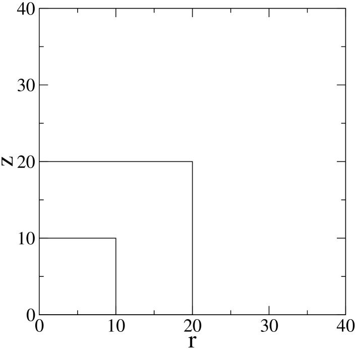
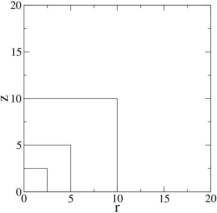
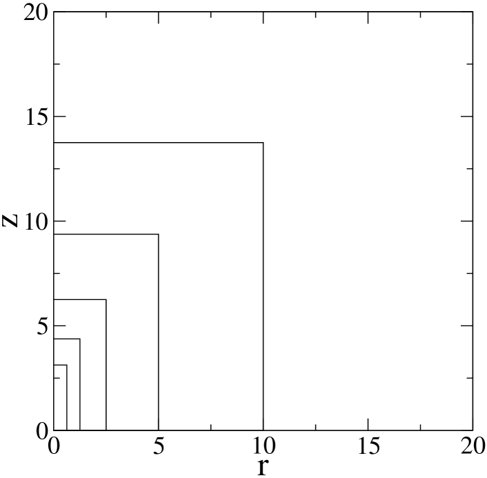
Figure 1: FMR grid hierarchies used for the Brill wave evolutions presented in this paper. Top left: $\sigma_{r}=\sigma_{z}=a=1$ (section 5.1); top right: $\sigma_{r}=\sigma_{z}=1$, $a=8.5$ (section 5.2), bottom: $\sigma_{r}=0.128$, $\sigma_{z}=1.6$, $a=325$ (section 5.3).

We run the simulation with three different resolutions, $N_{r}=N_{z}\in\{64,128,256\}$. This enables us to carry out a three-grid convergence test: for each variable $u$ we define a convergence factor

$$Q_{u}\equiv\frac{\parallel u_{4h}-u_{2h}\parallel}{\parallel u_{2h}-u_{h}\parallel},$$ (39)

with the indices referring to the grid spacing. The norms are discrete $L^{2}$ norms taken over the subsets of all grids in the FMR hierarchy that do not overlap with finer grids. For a second-order accurate numerical method we expect $Q_{u}=4$. Figure 2 confirms that the code is approximately second-order convergent. (Occasional values $Q_{u}>4$ are not uncommon in similar numerical schemes [4, 29].)

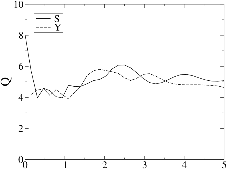
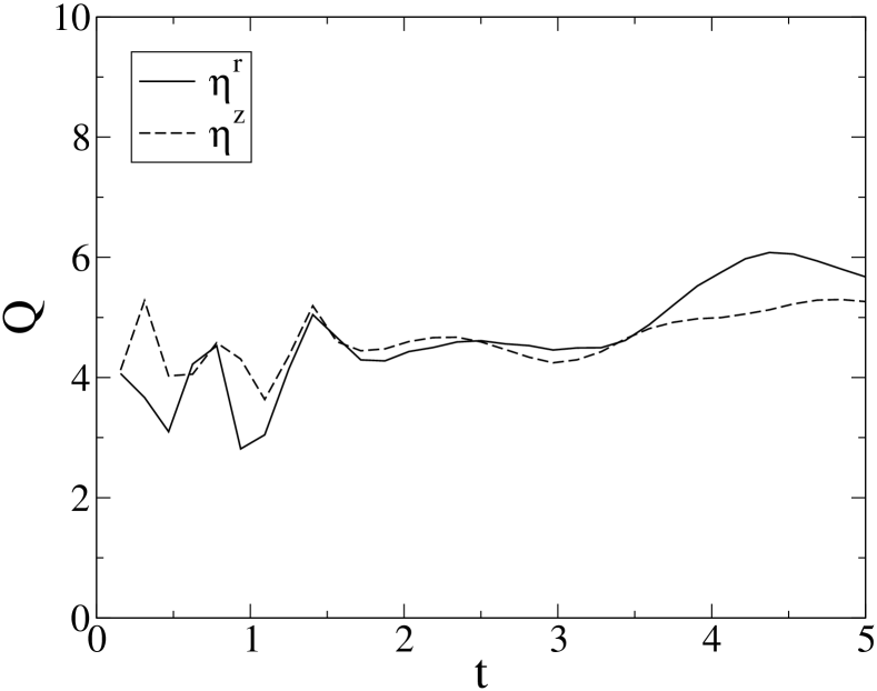
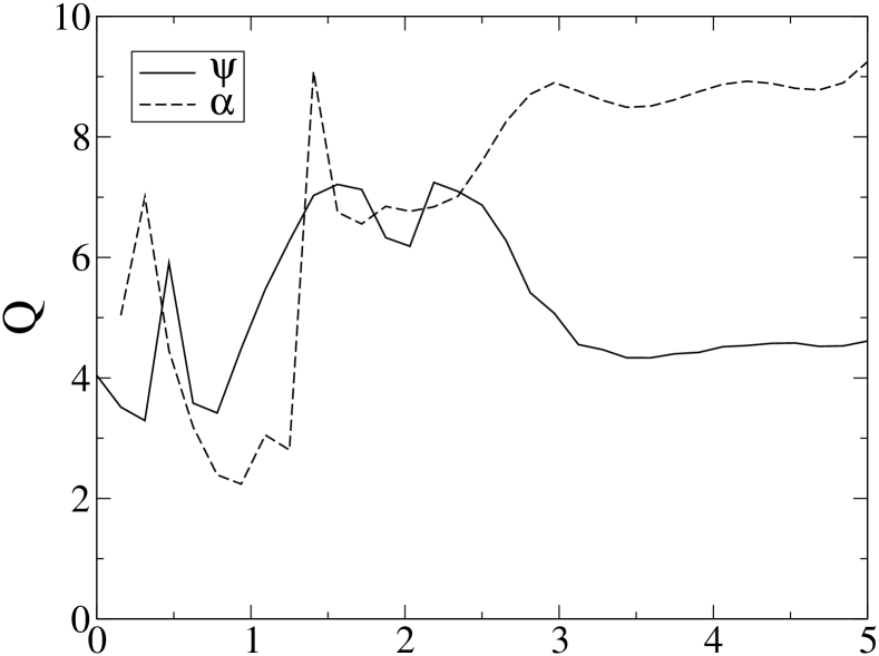
Figure 2: Three-grid convergence factors (39) for a Brill wave with $a=\sigma_{r}=\sigma_{z}=1$ computed from the three resolutions $N_{r}=N_{z}=64,\,128,\,256$.

As noted earlier, there are additional evolution equations for the variables $\eta_{+}$, $\eta_{-}$ and $\psi$ that are not actively evolved in our constrained evolution scheme. We use these to check the accuracy of the numerical implementation in the following way. We keep a set of auxiliary variables $\hat{\eta}_{+}$, $\hat{\eta}_{-}$ and $\hat{\psi}$ which are copied from their unhatted counterparts initially but evolved using the evolution equations (45)–(A). During the evolution, we form the differences between the two sets. Doing so for two different resolutions (grid spacings $h$ and $2h$) allows us to define another convergence factor for each $u\in\{\eta_{+},\eta_{-},\psi\}$ (referred to as residual convergence in the following),

$$q_{u}=\frac{\parallel\hat{u}_{2h}-u_{2h}\parallel}{\parallel\hat{u}_{h}-u_{h}\parallel}.$$ (40)

The results in figure 3 are again compatible with second-order convergence.

We note that the residual convergence test just presented is more severe than the three-grid convergence test in the following sense. For the residuals of the unsolved evolution equations to converge as desired, not only must the numerical solution be second-order convergent but the constraint and evolution equations and their boundary conditions must be compatible. No exact boundary conditions are known at a finite distance from the source and compatibility of the boundary conditions we use is only achieved at infinity. We deliberately chose the domain size in this convergence test to be sufficiently large ($\sim 10^{3}M_{\mathrm{ADM}}$) so that the effect of the boundary on the convergence factors $q_{u}$ is small.

As another consistency test, we compute a numerical approximation to the ADM mass. This is evaluated as a surface integral on a sphere close to the outer boundary, at spherical radius $R=R_{M}$,

$$M_{\mathrm{ADM}}=-R_{M}^{2}\int_{0}^{\pi/2}J_{A}n^{A}\,\sin\theta\,\rmd\theta,$$ (41)

where

$$J_{A}=2\psi_{,A}+\textstyle\frac{1}{2}rS_{,A},$$ (42)

$n_{A}$ is the unit normal in the spherical radial direction, and these expressions are valid in linearized theory. We evaluate $M_{\mathrm{ADM}}$ in (41) for two radii $R_{M}\in\{14,18\}$ and extrapolate to infinity assuming that $M_{\mathrm{ADM}}(R_{M})=M_{\mathrm{ADM}}(\infty)+\mathrm{const}/R_{M}$. The result in figure 3 shows how numerical conservation of the ADM mass improves with increasing resolution.

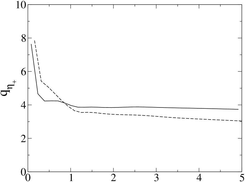
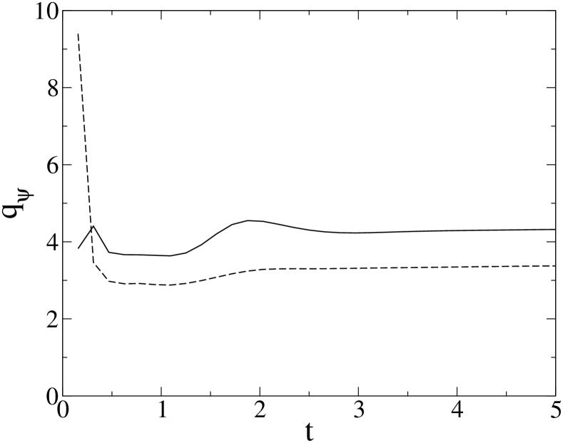
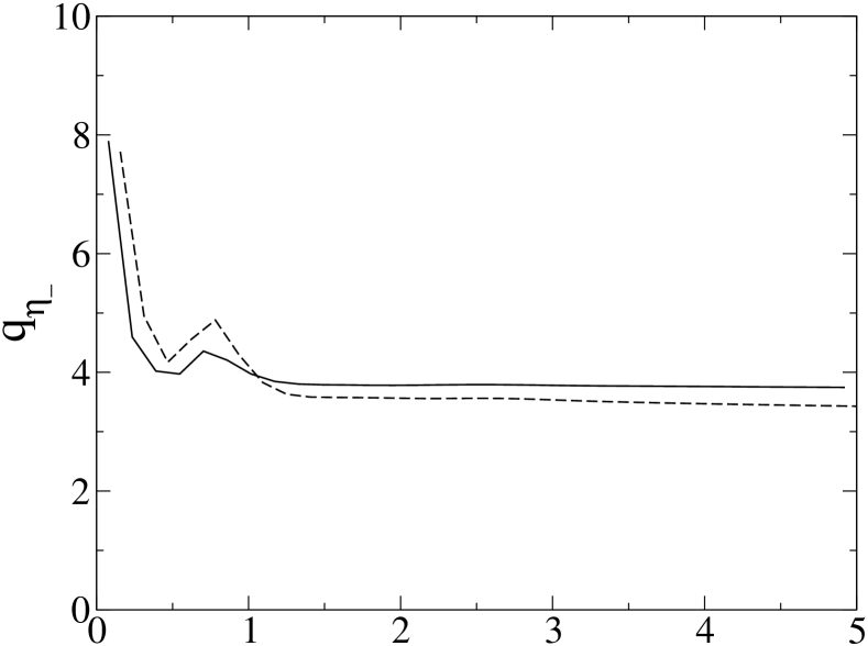
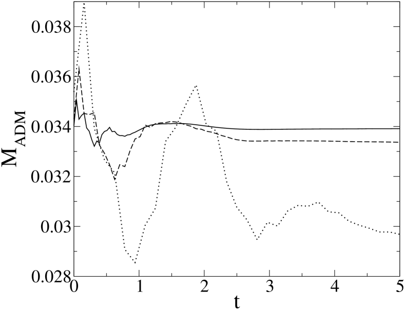
Figure 3: Residual convergence factors (40) for a Brill wave with $a=\sigma_{r}=\sigma_{z}=1$ computed from two pairs of resolutions, $N_{r}=N_{z}=64:128$ (dashed) and $128:256$ (solid). The bottom right panel shows the numerically computed ADM mass for the three different resolutions, $N_{r}=N_{z}=64$ (dotted), $128$ (dashed) and $256$ (solid).

5.2 “Spherical” collapse

Next we consider a wave with $\sigma_{r}=\sigma_{z}=1$ and $a=8.5$. We refer to this as “spherical” because $\sigma_{r}=\sigma_{z}$, although of course the actual wave is not spherically symmetric. Unlike the one in section 5.1, this wave is super-critical and will collapse to form a black hole. The ADM mass is $M_{\mathrm{ADM}}\approx 2$. We run the simulation for two different domain sizes, $r_{\mathrm{max}}=z_{\mathrm{max}}\in\{10,20\}.$ The FMR hierarchy is of a similar type as in section 5.1. On the smaller domain there are three grids and for the larger domain we add on another coarse grid (figure 1). We run the simulation with two different resolutions, $N_{r}=N_{z}\in\{128,256\}$. In [6], the same initial data were evolved on a non-uniform grid with spacing $\Delta r=\Delta z=1.92\times 10^{-2}$ close to the origin. This is comparable to our lower resolution grid hierarchy, which has grid spacing $\Delta r=\Delta z=1.95\times 10^{-2}$ on the finest grid.

Figure 4 shows the residual convergence factors defined in (40). The general trend is that the convergence factors are close to $4$ at late times but somewhat smaller at early times. Moving the outer boundary further out improves convergence considerably at early times, as can be seen particularly for the variables $\eta_{\pm}$. This demonstrates the effect of the outer boundary where imperfect boundary conditions are imposed at a finite distance. Because of the elliptic equations involved in our evolution scheme, inaccuracies in the outer boundary conditions influence the entire domain instantaneously, not only after the outgoing radiation interacts with the boundary as is the case in a hyperbolic scheme. Moving the outer boundary much further out by adding more coarse grids is not feasible for this evolution because of the computational cost involved in the current single-processor implementation of the code.

In particular, the value of the conformal factor $\psi$ far out appears to be very sensitive to the dynamics close to the origin. This is not the case for $\hat{\psi}$, which is evolved from the initial data by a hyperbolic PDE. As a result, the difference $\hat{\psi}-\psi$ has a large, spatially nearly constant contribution that is nearly resolution independent, thus causing the convergence factor $q_{\psi}$ to degrade.

At times later than those shown here, the convergence factors ultimately decrease because large gradients develop due to the grid-stretching property of maximal slicing. However, here we are only interested in the part of the evolution until just after the formation of the apparent horizon.

Figure 4 also indicates that both increasing the resolution and the boundary radius improves the numerical conservation of the ADM mass. For the larger domain at the higher resolution, the initial oscillations are at the $5\%$ level and after $t\approx 1$ the mass remains constant to within $1\%$.

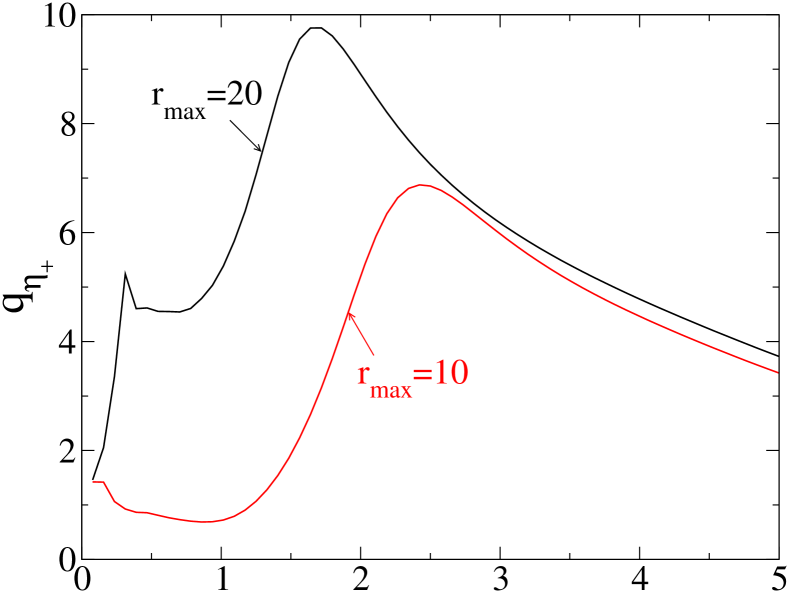
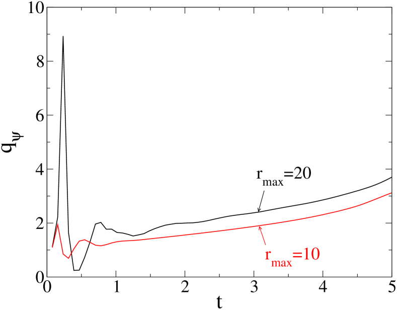
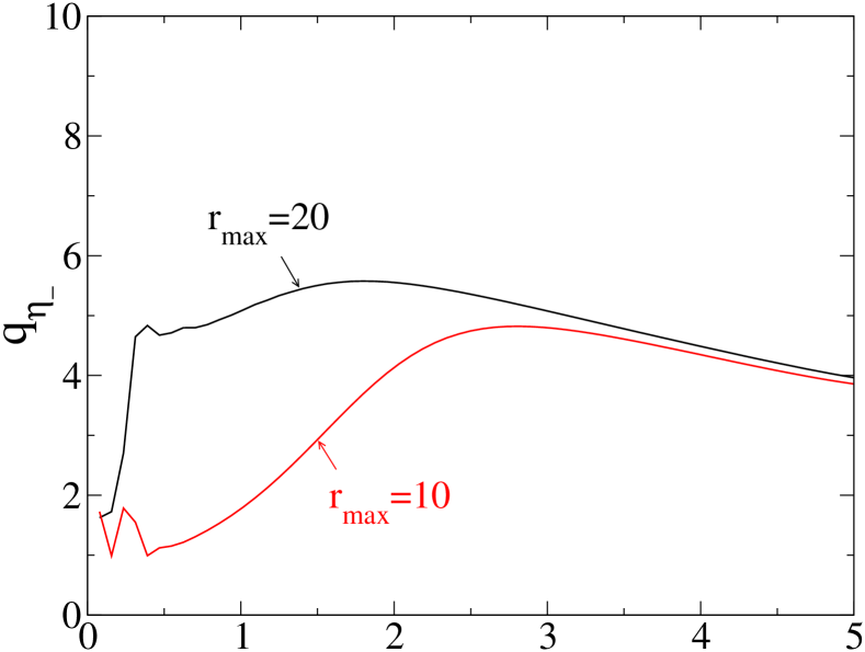
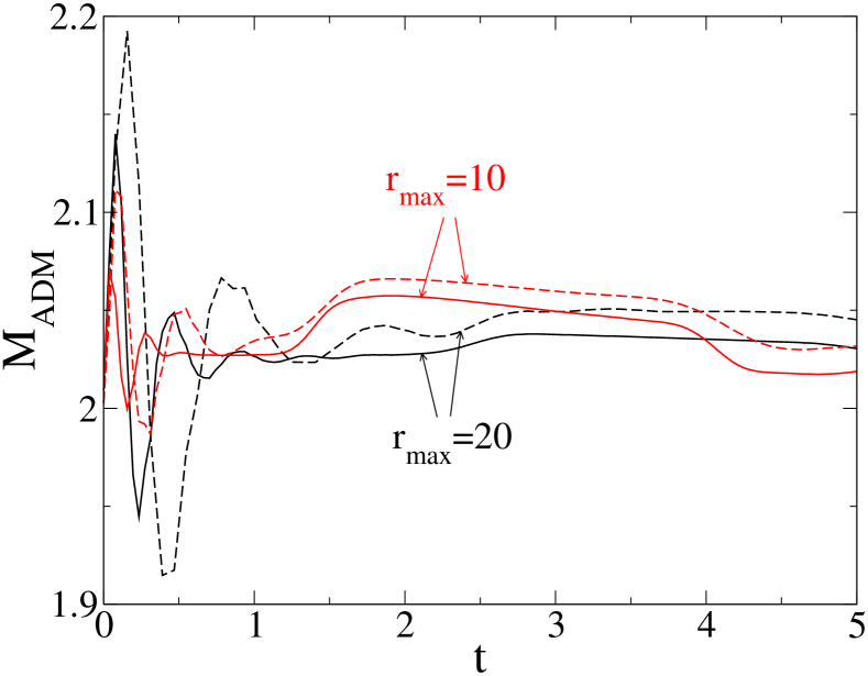
Figure 4: Residual convergence factors (40) for a Brill wave with $\sigma_{r}=\sigma_{z}=1$ and $a=8.5$, for two different domain sizes $r_{\mathrm{max}}=z_{\mathrm{max}}$. The bottom right panel shows the numerically computed ADM mass for the two different resolutions, $N_{r}=N_{z}=128$ (dashed) and $256$ (solid).

Next we evaluate the lapse function $\alpha$ in the origin $r=z=0$. As a consequence of the singularity avoidance property of maximal slicing, the lapse is expected to collapse towards zero as a strong-gravity region of spacetime is approached. Our result in figure (5) is in good agreement with [6] and appears to be insensitive to the resolution and boundary location.

We also plot the Riemann invariant $I=R^{abcd}R_{abcd}/16$ in the origin. The decay of this quantity after $t\approx 1$ agrees roughly with [6], although we find a somewhat different behaviour at earlier times (rather than increasing right from the beginning, $I$ first decreases for a short time). However there is a rather strong dependence on resolution and outer boundary location in this case, which indicates that the results for $I$ should be interpreted with care.

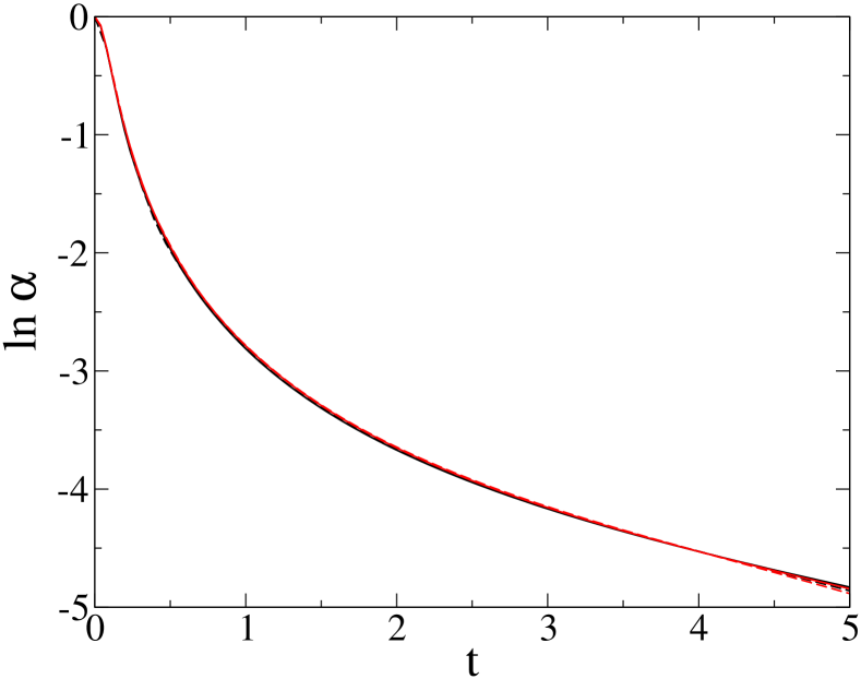
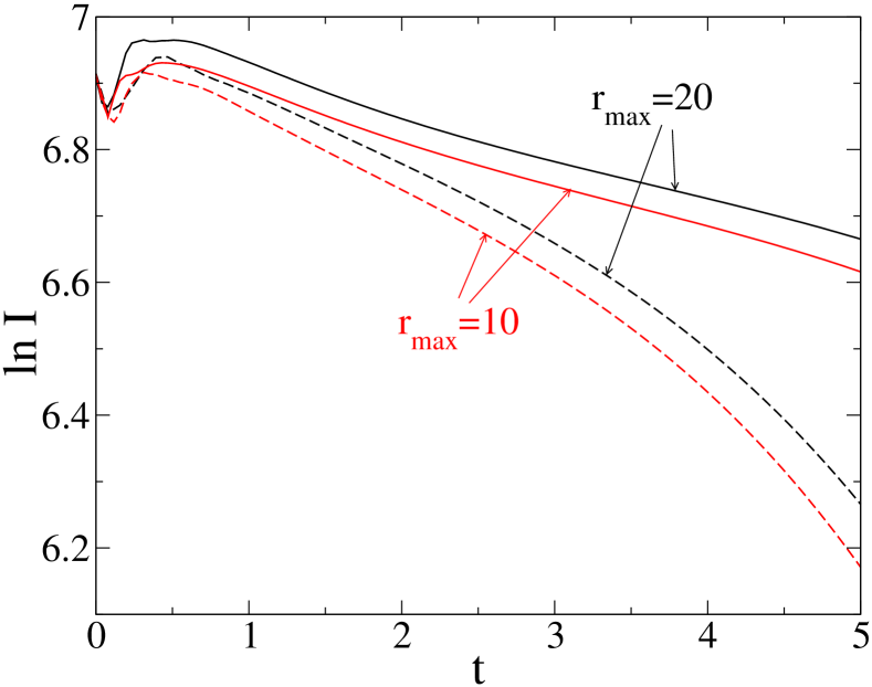
Figure 5: Lapse function $\alpha$ and Riemann invariant $I$ in the origin for a Brill wave with $\sigma_{r}=\sigma_{z}=1$ and $a=8.5$. Results for two different domain sizes $r_{\mathrm{max}}=z_{\mathrm{max}}$ and for two different resolutions $N_{r}=N_{z}=128$ (dashed) and $256$ (solid) are shown. (The four curves nearly coincide in the left plot.)

Finally we search for an apparent horizon. The evolution of the angle $\gamma_{\mathrm{max}}$ (cf. (37)) is shown in figure 6. It agrees reasonably well with [6], although we find that the horizon forms slightly earlier at $t=3.6\pm 0.2$ rather than at $t=3.9$. Also shown in figure 6 is the mass of the horizon, computed from its area $A_{\mathrm{AH}}=16\pi M_{\mathrm{AH}}^{2}$. When it first forms, the horizon has mass $M_{\mathrm{AH}}=1.85\pm 0.05$. The numerically computed ADM mass at this time is $M_{\mathrm{ADM}}=2.04\pm 0.02$ so that $M_{\mathrm{AH}}/M_{\mathrm{ADM}}=0.91\pm 0.03$, as compared with $M_{\mathrm{AH}}/M_{\mathrm{ADM}}=0.82$ reported in [6]. After its formation the horizon expands slightly (its mass increases by about $3\%$) and appears to ultimately settle down. The results stated here correspond to the run on the larger domain at the higher resolution and the errors are estimated by comparison with the other runs.

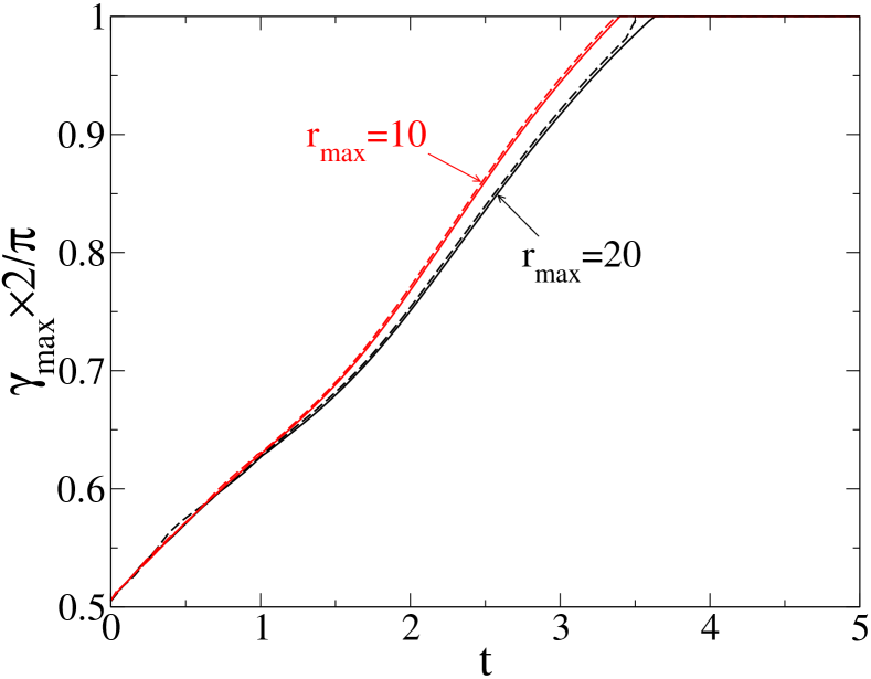
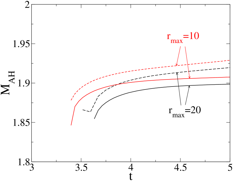
Figure 6: Apparent horizon finder angle $\gamma_{\mathrm{max}}$ (cf. (37)) and mass $M_{\mathrm{AH}}$ for a Brill wave with $\sigma_{r}=\sigma_{z}=1$ and $a=8.5$. Results for two different domain sizes $r_{\mathrm{max}}=z_{\mathrm{max}}$ and for two different resolutions $N_{r}=N_{z}=128$ (dashed) and $256$ (solid) are shown.

5.3 Highly prolate collapse

We now turn to a highly prolate Brill wave with $\sigma_{r}=0.128$, $\sigma_{z}=1.6$, and $a=325$, which again has $M_{\mathrm{ADM}}\approx 2$. This is one of the initial data sets considered in [16] and it was also evolved (until $t\approx 1.5$) in [6].

Our spatial domain has size $r_{\mathrm{max}}=z_{\mathrm{max}}=20$. The resolution on the base grid is taken to be $N_{r}=256$ and $N_{z}=64$. There are $6$ grids in the FMR hierarchy. Again all the grids contain the origin and the grid spacing is successively halved in both dimensions. The number of grid points $N_{r}$ in the radial direction is the same on all grids but $N_{z}$ is successively multiplied by a factor of (approximately) $1.34$. In this way the finer grids are better adapted to the prolate shape of the initial data. The grid hierarchy is shown in figure 1. The spacing on the finest grid is $\Delta r=2.44\times 10^{-3}$ and $\Delta z=9.77\times 10^{-3}$. By comparison, the grid used in [6] has $\Delta r=9.70\times 10^{-3}$ and $\Delta z=3.74\times 10^{-2}$ close to the origin, roughly four times coarser.

Figure 7 shows the evolution of the lapse function $\alpha$ and Riemann invariant $I$ in the origin. These agree well with [6], except for the $t\lesssim 0.5$ part of $I$ (but note the strong dependence of this quantity on resolution and outer boundary location apparent from figure 5).

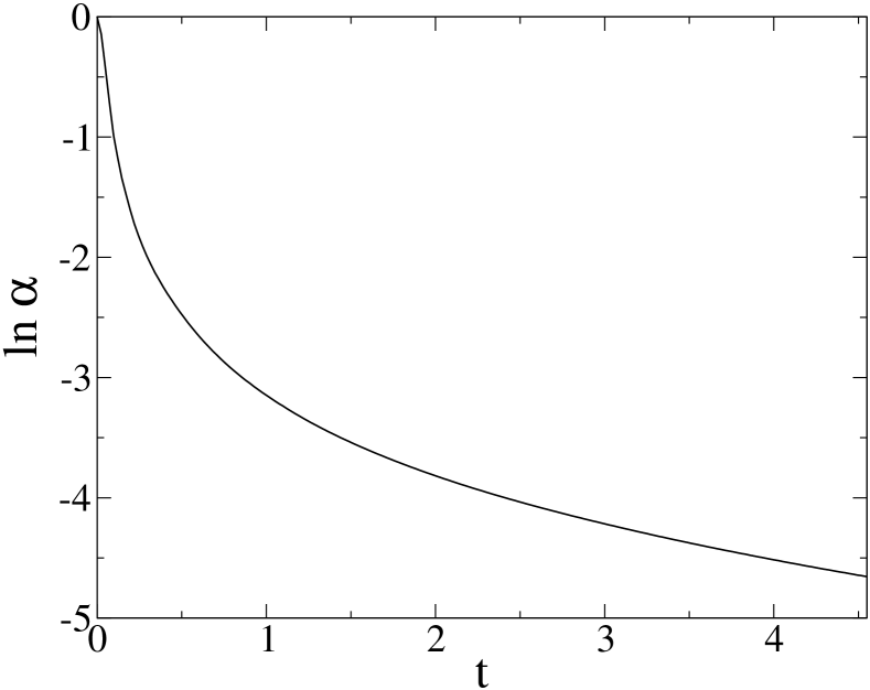
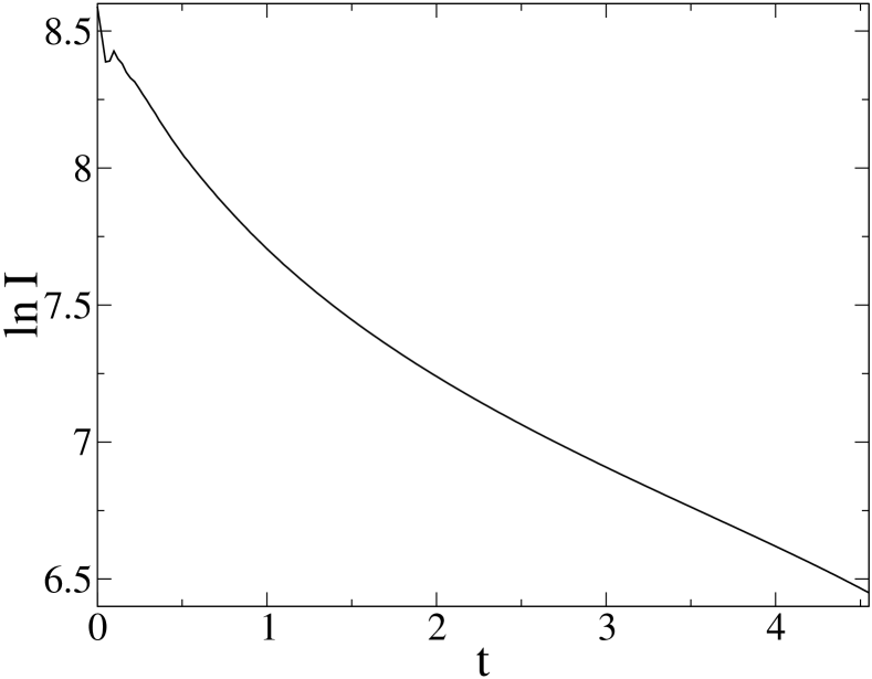
Figure 7: Lapse function $\alpha$ and Riemann invariant $I$ in the origin for a Brill wave with $\sigma_{r}=0.128$, $\sigma_{z}=1.6$ and $a=325$.

The approach to apparent horizon formation is shown in figure 8. We are able to evolve the wave for much longer than the authors of [6] and we confirm their conjecture that an apparent horizon will indeed form. It first appears at $t=3.9$ and its shape is remarkably close to a sphere in our coordinates. At its formation the apparent horizon has mass $M_{\mathrm{AH}}=1.990$ and at this time the ADM mass has settled down to a value of $M_{\mathrm{ADM}}=2.065$ so that $M_{\mathrm{AH}}/M_{\mathrm{ADM}}=0.96$. This is in accordance with the Penrose inequality [30], which conjectures that $M_{\mathrm{AH}}/M_{\mathrm{ADM}}\leqslant 1$.

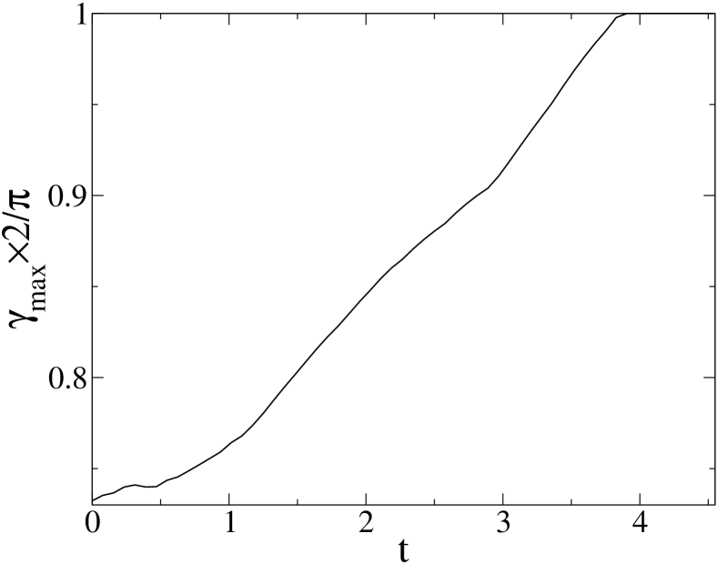
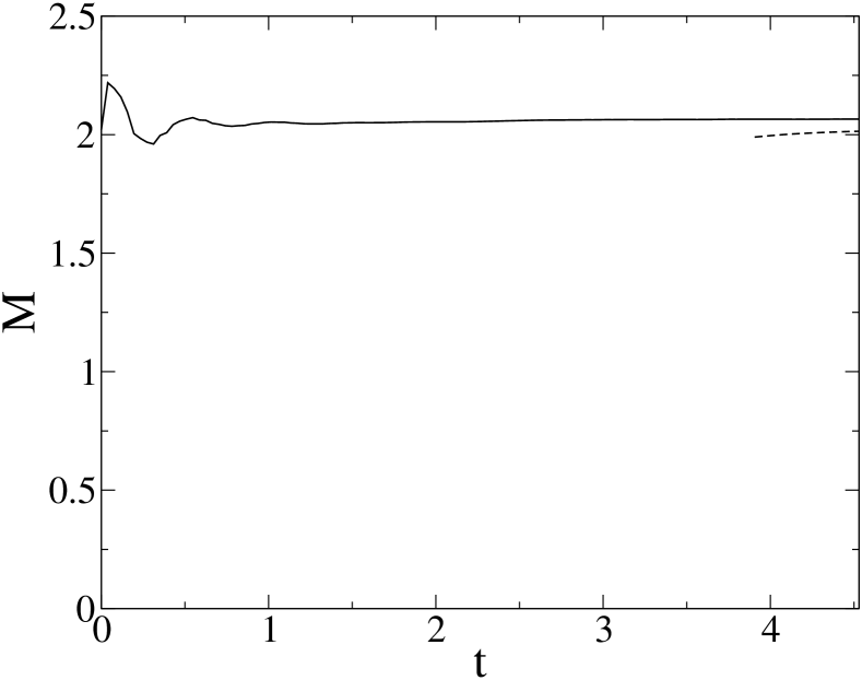
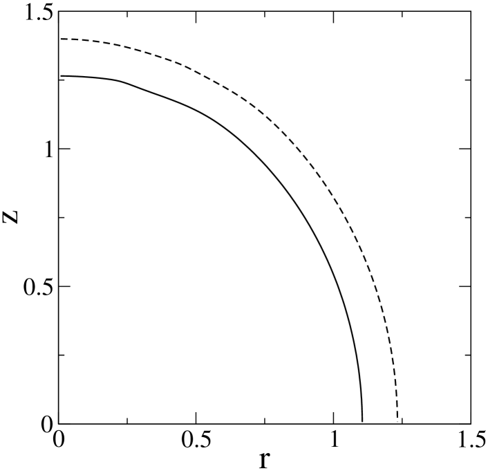
Figure 8: Apparent horizon formation for a Brill wave with $\sigma_{r}=0.128$, $\sigma_{z}=1.6$ and $a=325$. Top left: horizon finder angle $\gamma_{\mathrm{max}}$ (cf. (37)). Top right: ADM mass (solid) and apparent horizon mass (dashed). Bottom: coordinate location of the apparent horizon when it first forms at $t=3.9$ (solid), and at $t=4.5$ (dashed).

6 Conclusions

We considered constrained evolution schemes for the Einstein equations in axisymmetric vacuum spacetimes. One of the motivations for this work was to try and understand why the numerical elliptic solvers in some of these schemes, e.g. [4], failed to converge in certain situations. We found that this was related to the elliptic equations becoming indefinite. Apart from the implications for numerical convergence, we also pointed out that such equations might admit nonunique solutions. In section 3.3, we presented a new scheme that does not suffer from this problem. Its main features are a suitable rescaling of the extrinsic curvature with the conformal factor, and separate solution of the momentum constraints and isotropic spatial gauge conditions. Thus the scheme involves the solution of six elliptic equations rather than four as in [4]. Given that multigrid methods [19] can be used to solve these equations at linear complexity, this does not imply a severe increase in computational cost.

Our numerical implementation uses second-order accurate finite differences and combines mesh refinement with a multigrid elliptic solver, based on the algorithm of [29]. We work in cylindrical polar coordinates. Unlike in [6], we do not compactify the spatial domain but impose boundary conditions at a finite distance from the origin.

As an application of the code, we evolved Brill waves in section 5. We carried out a careful convergence test in section 5.1 and demonstrated that the code is approximately second-order convergent. For a stronger super-critical wave (section 5.2), convergence of the residuals of the unsolved evolution equations was somewhat slower at earlier times. Varying the domain size indicated that this is mainly caused by inaccuracies in the outer boundary conditions we use. These errors appear to have little effect on the formation of the apparent horizon.

In section 5.3, we evolved a highly prolate Brill wave. Such initial data were conjectured in [16] to form a naked singularity rather than a black hole, which would violate weak cosmic censorship. However an apparent horizon does form in our evolution. We thus improve on the results of the authors of [6], who could not evolve the wave for a sufficiently long time to see an apparent horizon form although they conjectured that this would happen eventually.

There are many directions in which this work could be extended. For simplicity we only considered vacuum spacetimes with a hypersurface-orthogonal Killing vector, i.e., vanishing twist. The addition of matter and twist should be straightforward. Care must be taken that the additional variables are rescaled with suitable powers of the conformal factor so that the Hamiltonian constraint (3.3) remains definite. An elegant framework capable of including twist is provided by the $(2+1)+1$ formalism [31, 32]. From a mathematical point of view, it would be interesting to prove that the Cauchy problem or even the initial-boundary value problem is well posed for the present (or a similar) formulation of the axisymmetric Einstein equations. These questions were studied for similar hyperbolic-elliptic systems in [33, 34, 35].

It is a disadvantage of constrained evolution schemes that inaccuracies in the outer boundary conditions influence the entire domain instantaneously. More work is needed on improved boundary conditions in the context of mixed hyperbolic-elliptic formulations of the Einstein equations. An alternative to an outer boundary at a finite distance would be the compactification towards spatial infinity used in [6]. However, outgoing waves ultimately fail to be resolved on such a compactified grid, which because of the elliptic equations involved has again adverse effects on the entire solution. This problem is avoided if hyperboloidal slices are used, which can be compactified towards future null infinity (see [36] for a related review article). In this case the constraint and evolution equations become formally singular at the boundary, which needs to be addressed in a numerical implementation.

On the computational side, the accuracy of the code could be improved by using fourth (or higher) order finite differences. Computational speed could be gained by parallelizing the code and running it on multiple processors.

It would be interesting to evolve even more prolate Brill waves than the one considered here. However the elliptic equations then become more and more anisotropic and the relaxation method employed in the multigrid method must be modified to ensure convergence. For the wave considered in this paper, line relaxation was found to accomplish this but we have not been able to achieve convergence for even more prolate configurations. More sophisticated modifications such as operator-based prolongation and restriction [28] are likely to be required. In any case, in order to evolve some of the extremely prolate initial data sets considered in [16] where $\sigma_{r}/\sigma_{z}\approx 10^{4}$ in (38), a radically different approach will probably be needed.

Another interesting application of our code would be Brill wave critical collapse. However, preliminary results indicate that we are currently unable to evolve waves close to the critical point for a sufficiently long time because reflections from the interior AMR grid boundaries become increasingly pronounced as more and more finer grids are added close to the origin. The mesh refinement algorithm of [29] that we adopt appeared to be sufficiently robust in the scalar field evolutions of [9, 10] but we suspect that the situation is quite different in vacuum collapse. An improved AMR algorithm for mixed hyperbolic-elliptic systems of PDEs will probably be required.

Appendix A Evolution equations

Here we list the evolution equations of the formulation of the axisymmetric Einstein equations presented in section 3.3. The variables $S$ and $\tilde{W}$ are actively evolved,

$$S_{,t}=\beta^{r}S_{,r}+\beta^{z}S_{,z}-\alpha\psi^{-6}\tilde{W}+r^{-1}\beta^{r}S+(r^{-1}\beta^{r})_{,r}\;,$$ (43)

$$\tilde{W}_{,t}=\beta^{r}\tilde{W}_{,r}+\beta^{z}\tilde{W}_{,z}+r^{-1}\eta_{+}\beta^{z}{}_{,r}-\alpha\psi^{2}\rme^{-2rS}\left[\alpha^{-1}(r^{-1}\alpha_{,r})_{,r}+2\psi^{-1}(r^{-1}\psi_{,r})_{,r}\right.$$

$$\left.+S_{,rr}+S_{,zz}+(r^{-1}S)_{,r}-r^{-1}R_{r}(A_{r}+2P_{r})+r^{-1}R_{z}(A_{z}+2P_{z})\right.$$

$$\left.-2r^{-1}P_{r}(2A_{r}+3P_{r})\right]$$

$$-\textstyle\frac{1}{2}\alpha\psi^{-6}r^{-1}[\eta_{+}^{2}+2\eta_{-}r\tilde{W}-4(r\tilde{W})^{2}]+4r^{-1}\beta^{r}\tilde{W}.$$ (44)

The variables $\psi$ and $\eta^{A}$ are not evolved but solved for using the constraint equations. However the Einstein equations also imply the following evolution equations that may be used to check the accuracy of a numerical scheme.

$$\psi_{,t}=\beta^{r}\psi_{,r}+\beta^{z}\psi_{,z}+\textstyle\frac{1}{2}r^{-1}\beta^{r}\psi-\textstyle\frac{1}{6}\alpha\psi^{-5}(\eta_{-}-2r\tilde{W}),$$ (45)

$$\eta_{+,t}=2\alpha\psi^{2}\rme^{-2rS}[-\alpha^{-1}\alpha_{,rz}-2\psi^{-1}\psi_{,rz}+R_{r}A_{z}+R_{z}(A_{r}+r^{-1})+6P_{r}P_{z}$$

$$+2P_{r}(A_{z}+R_{z})+2P_{z}(A_{r}+R_{r})]$$

$$+\beta^{r}(\eta^{r}{}_{,rz}+\eta^{z}{}_{,rr}+3r^{-1}\eta_{+})+\beta^{z}(\eta^{r}{}_{,zz}+\eta^{z}{}_{,rz})-\eta_{+}\beta_{-}$$

$$+\textstyle\frac{2}{3}(\beta^{r}{}_{,z}-2\beta^{z}{}_{,r})\eta_{-}+\textstyle\frac{2}{3}r\tilde{W}\beta_{+}+\textstyle\frac{1}{3}\alpha\psi^{-6}\eta_{+}(\eta_{-}+4r\tilde{W}),$$ (46)

$$\eta_{-,t}=\alpha\psi^{2}\rme^{-2rS}[-\alpha^{-1}\alpha_{,rr}+\alpha^{-1}\alpha_{,zz}-2\psi^{-1}\psi_{,rr}+2\psi^{-1}\psi_{,zz}+2R_{r}(A_{r}+r^{-1})$$

$$-2A_{z}R_{z}+2P_{r}(2A_{r}+3P_{r}+2R_{r})-2P_{z}(2A_{z}+3P_{z}+2R_{z})]$$

$$+\beta^{r}(\eta^{r}{}_{,rr}-\eta^{z}{}_{,rz}+3r^{-1}\eta_{-})+\beta^{z}(\eta^{r}{}_{,rz}-\eta^{z}{}_{,zz})$$

$$-\textstyle\frac{2}{3}\beta_{-}(2\eta_{-}-r\tilde{W})+(\beta^{z}{}_{,r}-\beta^{r}{}_{,z})\eta_{+}+\textstyle\frac{1}{3}\alpha\psi^{-6}\eta_{-}(\eta_{-}+4r\tilde{W}).$$ (47)

Appendix B Finite-difference operators and boundary conditions

Centred second-order accurate finite-difference operators are used at all interior grid points. We only give the expressions for derivatives in the $r$ direction; corresponding expressions hold in the $z$ direction. The symbol $\approx$ denotes equality up to $\Or(\Delta r)^{2}$.

$$u_{,r}|_{i} \approx (u_{i+1}-u_{i-1})/(2\Delta r),$$

$$(r^{-1}u)_{,r}|_{i} \approx (u_{i+1}/r_{i+1}-u_{i-1}/r_{i-1})/(2\Delta r),$$

$$u_{,rr}|_{i} \approx (u_{i+1}-2u_{i}+u_{i-1})/(\Delta r)^{2},$$

$$(r^{-1}u_{,r})_{,r}|_{i} \approx [(u_{i+2}-u_{i})/r_{i+1}-(u_{i}-u_{i-2})/r_{i-1}]/[4(\Delta r)^{2}].$$ (48)

At $r=0$ ($z=0$), a Dirichlet condition is imposed if the variable is an odd function of $r$ ($z$) and a Neumann condition if it is an even function of $r$ ($z$). The parities of the various variables are as follows,

$$\textrm{odd in }r: \beta^{r},\eta^{r},S,\tilde{W}$$

$$\textrm{even in }r: \alpha,\psi,\beta^{z},\eta^{z}$$

$$\textrm{odd in }z: \beta^{z},\eta^{z}$$

$$\textrm{even in }z: \alpha,\psi,\beta^{r},\eta^{r},S,\tilde{W}$$ (49)

The value of a variable $u$ at the ghost point is set to be $u_{0}=-u_{1}$ if $u$ obeys a Dirichlet condition and $u_{0}=u_{1}$ if it obeys a Neumann condition. This discretization at the boundary is second-order accurate.

Dirichlet conditions at the outer boundary are implemented in a similar way. In order to impose the falloff condition (35), we note that $Ru$ is a linear function of $R$ and so we linearly extrapolate $Ru$ in the radial direction from the interior grid points to the ghost points in order to find the values of $u$ there. The Sommerfeld condition (36) is rewritten in the form

$$Ru_{,t}+ru_{,r}+zu_{,z}+u-u_{\infty}=0$$ (50)

and discretized at the outer ghost points on the base grid of the AMR hierarchy in order to integrate the values of $u$ there forward in time. Here backward differencing is used in the direction normal to the boundary,

$$u_{,r}|_{i}\approx(3u_{i}-4u_{i-1}+u_{i-2})/(2\Delta r)$$ (51)

and similarly in the $z$ direction.

References

References

- [1] Wilson J R 1979 A numerical method for relativistic hydrodynamics Sources of Gravitational Radiation ed Smarr L L (Cambridge University Press) pp 423–445
- [2] Bardeen J and Piran T 1983 General relativistic axisymmetric rotating systems: Coordinates and equations Phys. Rep. 96 205–250
- [3] Evans C R 1986 An approach for calculating axisymmetric gravitational collapse Dynamical Spacetimes and Numerical Relativity ed Centrella J M (Cambridge University Press) pp 3–39
- [4] Choptuik M W, Hirschmann E W, Liebling S L and Pretorius F 2003 An axisymmetric gravitational collapse code Class. Quantum Grav. 20 1857–1878
- [5] Abrahams A M and Evans C R 1993 Critical behavior and scaling in vacuum axisymmetric gravitational collapse Phys. Rev. Lett. 70 2980–2983
- [6] Garfinkle D and Duncan G C 2001 Numerical evolution of Brill waves Phys. Rev. D 63 044011
- [7] Brill D R 1959 On the positive mass of the Bondi-Weber-Wheeler time-symmetric gravitational waves Ann. Phys. 7 466–483
- [8] Abrahams A M and Evans C R 1994 Universality and scaling in axisymmetric vacuum collapse Phys. Rev. D 49 3998–4003
- [9] Choptuik M W, Hirschmann E W, Liebling S L and Pretorius F 2003 Critical collapse of the massless scalar field in axisymmetry Phys. Rev. D 68 044007
- [10] Choptuik M W, Hirschmann E W, Liebling S L and Pretorius F 2004 Critical collapse of a complex scalar field with angular momentum Phys. Rev. Lett. 93 131101
- [11] Shapiro S L and Teukolsky S A 1991 Formation of naked singularities: The violation of cosmic censorship Phys. Rev. Lett. 66 994–997
- [12] Barnes A 2004 Numerical Relativistic Hydrodynamics in Planar and Axisymmetric Spacetimes PhD thesis University of Cambridge
- [13] Rinne O 2005 Axisymmetric Numerical Relativity PhD thesis University of Cambridge (E-print http://www.arxiv.org/abs/gr-qc/0601064)
- [14] Pfeiffer H P and York Jr J W 2005 Uniqueness and nonuniqueness in the Einstein constraints Phys. Rev. Lett. 95 091101
- [15] Walsh D M 2007 Non-uniqueness in conformal formulations of the Einstein constraints Class. Quantum Grav. 24 1911–1925
- [16] Abrahams A M, Heiderich K R, Shapiro S L and Teukolsky S A 1992 Vacuum initial data, singularities, and cosmic censorship Phys. Rev. D 46 2452–2463
- [17] Gilbarg D and Trudinger N S 1977 Elliptic Partial Differential Equations of Second Order (Springer)
- [18] Stoer J and Bulirsch R 2002 Introduction to Numerical Analysis 2nd ed (Springer)
- [19] Brandt A 1977 Multilevel adaptive solutions to boundary value problems Math. Comput. 31 333–390
- [20] Elman H C, Ernst O G and O’Leary D P 2001 A multigrid method enhanced by Krylov subspace iteration for discrete Helmholtz equations SIAM J. Sci. Comput. 23 1291–1315
- [21] Cordero-Carrión I, Ibáñez J M, Gourgoulhon E, Jaramillo J L and Novak J 2008 Mathematical issues in a fully-constrained formulation of Einstein equations Phys. Rev. D 77 084007
- [22] York Jr J W 1979 Kinematics and dynamics of general relativity Sources of gravitational radiation ed Smarr L L (Cambridge University Press) pp 83–126
- [23] Brill D and Cantor M 1981 The Laplacian on asymptotically flat manifolds and the specification of scalar curvature Composit. Math. 43 317–330
- [24] Pfeiffer H P and York Jr J W 2003 Extrinsic curvature and the Einstein constraints Phys. Rev. D 67 044022
- [25] Berger M J and Oliger J 1984 Adaptive mesh refinement for hyperbolic partial differential equations J. Comput. Phys. 53 484–512
- [26] Rinne O and Stewart J M 2005 A strongly hyperbolic and regular reduction of Einstein’s equations for axisymmetric spacetimes Class. Quantum Grav. 22 1143–1166
- [27] Kreiss H O and Oliger J 1973 Methods for the approximate solution of time dependent problems Global Atmospheric Research Programme (Publication Series No. 10)
- [28] Trottenberg U, Oosterlee C W and Schüller A 2001 Multigrid (Academic Press)
- [29] Pretorius F and Choptuik M W 2006 Adaptive mesh refinement for coupled elliptic-hyperbolic systems J. Comput. Phys. 218 246–274
- [30] Penrose R 1973 Naked singularities Ann. N. Y. Acad. Sci. 224 125–134
- [31] Geroch R 1971 A method for generating solutions of Einstein’s equations J. Math. Phys. 12 918–924
- [32] Maeda K, Sasaki M, Nakamura T and Miyama S 1980 A new formulation of the Einstein equations for relativistic rotating systems Prog. Theor. Phys. 63 719–721
- [33] Choquet-Bruhat Y and York Jr J W 1996 Mixed elliptic and hyperbolic systems for the Einstein equations Gravitation, Electromagnetism and Geometric Structures ed Ferrarese G (Bologna: Pythagora Editrice) pp 55–73
- [34] Andersson L and Moncrief V 2003 Elliptic-hyperbolic systems and the Einstein equations Ann. H. Poincaré 4 1–34
- [35] Nagy G and Sarbach O 2006 A minimization problem for the lapse and the initial-boundary value problem for Einstein’s field equations Class. Quantum Grav. 16 S477–S504
- [36] Frauendiener J 2004 Conformal infinity Living Rev. Relativity 7(1)