Universal intermittent properties of particle trajectories in highly turbulent flows

Abstract

We present a collection of eight data sets, from state-of-the-art experiments and numerical simulations on turbulent velocity statistics along particle trajectories obtained in different flows with Reynolds numbers in the range $R_{\lambda}\in[120:740]$. Lagrangian structure functions from all data sets are found to collapse onto each other on a wide range of time lags, pointing towards the existence of a universal behaviour, within present statistical convergence, and calling for a unified theoretical description. Parisi-Frisch Multifractal theory, suitable extended to the dissipative scales and to the Lagrangian domain, is found to capture intermittency of velocity statistics over the whole three decades of temporal scales here investigated.

Understanding the statistical properties of particle tracers advected by turbulent flows is a challenging theoretical and experimental problem FS.06 ; LPVCAB.01 . It is a key ingredient for the development of stochastic models Po.00 ; lamorgese07 , in such diverse contexts as turbulent combustion, industrial mixing, pollutant dispersion and cloud formation Shaw.03 . The main difficulty of Lagrangian investigations, following particle trajectories, stems from the necessity to resolve the wide range of time scales driving different particle behaviours: from the longest, $T_{L}$, given by the stirring mechanism, to the shortest $\tau_{\eta}$, typical of viscous dissipation. Indeed the ratio, $T_{L}/\tau_{\eta}\sim R_{\lambda}$, grows with the Taylor Reynolds number, $R_{\lambda}$, that varies up to few thousands in laboratory flows. Some aspects of Lagrangian statistics have been experimentally measured: particle accelerations LPVCAB.01 , velocity fluctuations in the inertial range MMMP.01 ; X06 and two-particle dispersion berg ; B06 . Others, connected to the entire range of motions, have long been restricted to numerical simulations BBCLT.05 ; MLP04 ; pkyeung ; mueller ; BBCDLT.04 . A fundamental open question is connected to intermittency, i.e. the observed strong deviations from Gaussian statistics, becoming larger and larger when considering fluctuations at smaller and smaller scales. Besides, the dependency of velocity statistics at various temporal scales on large scale forcing and boundary conditions is the so-called problem of universality. Thus, universality features are linked to the degree of anisotropy and non-homogeneities of turbulent statistics bp.physrep . Similar problems have already been explored measuring the velocity fluctuations in the laboratory frame (Eulerian statistics), where clear evidence of universality have been obtained ArETAL.96 .
To build a general theory of turbulent statistics, universality is the first requirement and, if proved, may open the possibility for effective stochastic modeling Sawford91 in many applied situations.
This Letter aims at investigating intermittency and universality properties of velocity temporal fluctuations by quantitatively comparing data obtained from the most advanced laboratory berg ; MMMP.01 ; X06 and numerical BBCLT.05 ; MLP04 ; mueller ; pkyeung ; chicago experiments. Main outcomes of our analysis are twofold. First, we show that data collapse on a common functional form, providing evidence for universality of velocity fluctuations –up to moments currently achievable with high statistical accuracy. At intermediate and inertial scales, data show an intermittent behaviour. Second, we propose a stochastic phenomenological modelisation in the entire range of scales, using a Multifractal description linking Eulerian and Lagrangian statistics.

We analyse the probability distribution of velocity fluctuations at all scales, focusing on moments of these distributions, namely the Lagrangian Velocity Structure Functions (LVSF) of positive integer order $p$:

$$S_{i}^{(p)}(\tau)=\langle[v_{i}(t+\tau)-v_{i}(t)]^{p}\rangle=\langle(\delta_{\tau}v_{i})^{p}\rangle,$$ (1)

where $i=x,y,z$ are the velocity components along a single particle path, and the average is defined over the ensemble of trajectories. As stationarity and homogeneity is assumed, moments of velocity increments only depend on the time lag $\tau$. In the inertial range, for $\tau_{\eta}\ll\tau\ll T_{L}$, non-linear energy transfer governs the dynamics. Thus, from a dimensional viewpoint, only the scale $\tau$ and the average energy dissipation rate for unit mass $\epsilon$ should matter for the structure function behaviour. The only admissible choice is $S_{i}^{(p)}(\tau)\sim(\epsilon\tau)^{p/2}$, but it does not take into account the fluctuating nature of energy dissipation. Empirical studies have indeed shown that the tails of the probability density functions of $\delta_{\tau}v$ become increasingly non-Gaussian at decreasing $\tau/T_{L}$. In terms of moments of the velocity fluctuations, intermittency reveals itself in the anomalous scaling exponents, i.e. a breakdown of the dimensional law for which we have that

$$S_{i}^{(p)}(\tau)\sim\tau^{\xi(p)}\,,$$ (2)

with $\xi(p)\neq p/2$. Notice that when dissipative effects dominate, typically for scales $\tau\sim\tau_{\eta}$ and smaller, the power-law behaviour (2) is no longer valid, and refined arguments have to be employed, as we will see in the following.

EXP	$R_{\lambda}$	$\tau_{\eta}$ ($s$)	meas. vol. ($\eta^{3}$)	$N_{tr}$	Tech.	Ref.
1	124	$8.5\times 10^{-2}$	$340^{3}$	$1.6\times 10^{6}$	PTV	[8]
2	690	$9\times 10^{-4}$	$1700^{3}$	$6.0\times 10^{6}$	PTV	[7]
3	740	$2\times 10^{-4}$	$6600^{3}$	$9.5\times 10^{3}$	AD	[6]

Table 1: Experiments. By columns: 1- experiment label; 2- Taylor Reynolds number; 3- Kolmogorov time scale $\tau_{\eta}$; 4- measurement volume in unit of the Kolmogorov length scale $\eta$; 5- $N_{tr}$ total number of Lagrangian trajectories measured; 6- measurement technique: Particle Tracking Velocimetry (PTV) and Acoustic Doppler (AD); 7- Reference where information on the way the corresponding dataset was obtained can be found.

DNS	$R_{\lambda}$	$N^{3}$	$N_{tr}$	Diss.	Tech.	Ref.
1	140	$256^{3}$	$5\times 10^{5}$	N	T	[11]
2	320	$1024^{3}$	$5\times 10^{6}$	N	T	[13]
3	400	$2048^{3}$	$3\times 10^{5}$	N	L	[10]
4	600	$1856^{3}$	$1.6\times 10^{7}$	C	L	[18]
5	650	$2048^{3}$	$4\times 10^{5}$	N	CS	[12]

Table 2: Direct numerical simulations. By columns: 1- numerical simulation label; 2- Taylor Reynolds number $R_{\lambda}$; 3- number of collocation points $N^{3}$; 4- total number of Lagrangian tracers $N_{p}$; 5- characteristic of dissipation: normal viscous terms (N), weakly compressible code (C); 6- interpolation technique for Lagrangian integration: linear interpolation (L), tricubic interpolation (T); cubic-splines (CS); 7- Reference where information on the way the corresponding dataset was obtained can be found.

The statistics of velocity fluctuations at varying time lag $\tau$ can be quantitatively captured by the logarithmic derivatives of $S_{i}^{(p)}(\tau)$ versus $S_{i}^{(2)}(\tau)$ ess ; LM.04 ; PoF.07 . This defines the local scaling exponents

$$\zeta_{i}(p,\tau)=\frac{{\rm d}\log S_{i}^{(p)}(\tau)}{{\rm d}\log S_{i}^{(2)}(\tau)}\,.$$ (3)

For statistically isotropic turbulence, all components are equivalent, so that their spread quantifies the degree of anisotropy present in teh flow. The $\tau$-dependence of $\zeta_{i}(p,\tau)$ allows for a scale-by-scale characterisation of intermittency.

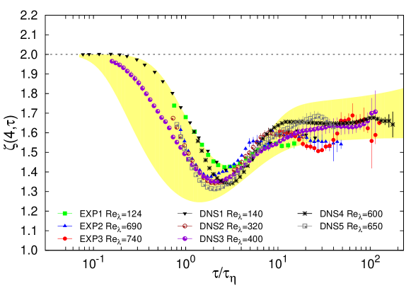
Figure 1: (Color online) Log-Lin plot of the fourth order local exponent, $\zeta(4,\tau)$, averaged over velocity components, as a function of the normalised time lag $\tau/\tau_{\eta}$. Data sets come from three experiments (EXP) (see Table 1) and five direct numerical simulations (DNS) (see Table 2). Error bars are estimated from the spread between the three components, except in EXP3 where only two components were measured. Each data set is plotted only in the time range where recognised experimental/numerical limitations are not affecting the results. In particular, for each data set, the largest time lag always satisfies $\tau<T_{L}$. The minimal time lag is set by the highest fully resolved frequency. The shaded area displays the prediction obtained by the MF model by using $D_{Lo}(h)$ or $D_{Tr}(h)$, with $\beta=4$, for a range of $R_{\lambda}\in[150:800]$, comparable with the range of $R_{\lambda}$ in the data. Notice that the MF predictions have been obtained by fixing equal to $7$, the multiplicative constant in the definition of $\tau_{\eta}$. The straight dashed line corresponds to the dimensional non-intermittent value $\zeta(4,\tau)=2$, achieved at small time lags where structure functions do become differentiable. Notice that two among the DNS are sufficiently resolved to get the mentioned dimensional scaling in the high frequency limit.

Figure 1 shows the local exponents of order $p=4$ from a collection of eight data sets, see Table I and II, for different Reynolds numbers. Most of these data sets are new, as well as completely new is the performed analysis, here presented. We focused on the fourth order moment, since it is the highest order achievable with statistical convergence for all data sets. Two observations can be done. First, all data sets show a similar strong variation around the dissipative time $\tau/\tau_{\eta}\sim O(1)$ that depends on the Reynolds number, and then a clear tendency toward a plateau for larger lags $\tau>10\tau_{\eta}$. Second, all data sets, with comparable Reynolds numbers, well agree in the whole range of time lags. The relative scatter increases only for large $\tau$, due to the combined effects of the lack of statistics, the anisotropy of the flows and the different valus of $R_{\lambda}$. In particular, finite volume effects in experimental particle tracking can produce a small – but systematic – downward shift of the points at long-lag times ott_mann ; PoF.07 . It is worth noticing that error bars estimated from anisotropic contributions decrease by going to small $\tau$, indicating that isotropy tends to be recovered at sufficiently small scales, i.e. large scale anisotropic contributions becomes less and less important. In addition, the fact that, at comparable Reynolds numbers, all data sets recover the same behaviour by going to smaller and smaller time lags provides a clear indication of Lagrangian universality of the energy cascade. Such an agreement has not been observed before and is comparable with that found for the corresponding Eulerian quantities ArETAL.96 .
The quality of data shown in (Fig. 1) opens the possibility to quantitatively test phenomenological models for LVSF, scale-by-scale. Parisi-Frisch Multifractal (MF) model of the inertial range Fr.95 , and its generalization to the dissipative range PV.87 ; Ne.90 ; FV.91 ; meneveau , has proved to give a satisfactory description of Eulerian and Lagrangian fluctuations Bo.93 ; bof02 ; CRLMPA.03 ; BBCDLT.04 . It is thus appealing to search for a link between Eulerian and Lagrangian statistics Bo.93 ; bof02 ; CRLMPA.03 ; BBCDLT.04 , since this points to a unique interpretation of turbulent fluctuations. Moreover, it would reduce the number of free parameters. According to the MF model, Eulerian velocity increments at inertial scales are characterised by a local Hölder exponent $h$, i.e. $\delta_{r}u\sim r^{h}$, whose probability ${\cal P}(h)\sim r^{3-D(h)}$ is weighted by the Eulerian fractal dimension $D(h)$ of the set where $h$ is observed Fr.95 . The dimensional relation $\tau\sim r/\delta_{r}u$ bridges Lagrangian fluctuations over a time lag $\tau$ to the Eulerian ones at scale $r$. Following Refs. Bo.93 ; meneveau , it is shown in Ref. CRLMPA.03 how to extend the MF framework to get a unified description at all time scales for Lagrangian turbulence. Accordingly, Lagrangian increments display a continuous and differentiable behaviour at the transition from the dissipative to the inertial range,

$$\delta_{\tau}v(h)=V_{0}\,\frac{\tau}{T_{L}}\left[\left(\frac{\tau}{T_{L}}\right)^{\beta}+\left(\frac{\tau_{\eta}}{T_{L}}\right)^{\beta}\right]^{\frac{2h-1}{\beta(1-h)}}\,,$$ (4)

$\beta$ being a free parameter controlling the crossover around $\tau\!\sim\!\tau_{\eta}$, and $V_{0}$ the root mean square velocity. In order to get a prediction for the behaviour of the LVSF, given by

$$\langle(\delta_{\tau}v)^{p}\rangle\sim\int dhP_{h}(\tau,\tau_{\eta})[\delta_{\tau}v(h)]^{p}\,,$$ (5)

we have to consider, in (4), the intermittent fluctuations of the dissipative scale Bo.93 ; CRLMPA.03 ; BBCDLT.04 , $\tau_{\eta}(h)/T_{L}\!\sim\!R_{\lambda}^{2(h\!-\!1)/(1\!+\!h)}$. The last necessary ingredient is to specify the probability of observing fluctuations of $h$. This is done in analogy to Eq. (4):

$$P_{h}(\tau,\tau_{\eta})={\cal Z}^{-1}(\tau)\left[\left(\frac{\tau}{T_{L}}\right)^{\beta}+\left(\frac{\tau_{\eta}}{T_{L}}\right)^{\beta}\right]^{\frac{3-D(h)}{\beta(1-h)}},$$ (6)

where ${\cal Z}$ is a normalizing function CRLMPA.03 and $D(h)$ the fractal dimension of the support of the exponents $h$. Once specified the Reynolds number, we are left with two parameters - the expoent $\beta$ and a multiplicative constant in the definition of $\tau_{\eta}$ -, while the function $D(h)$ comes from the knowledge of the Eulerian statistics.
Eulerian Velocity Structure Functions (EVSF) have been measured in the last two decades (see Ref.ArETAL.96 for a data collection) providing a way to estimate the function $D(h)$ based on empirical data. Many functional forms have been proposed in the literature Fr.95 that are consistent with data, up to statistical uncertainties. Eulerian velocity statistics can be measured in terms of longitudinal or transverse fluctuations. Fluid velocity along particle paths is naturally sensitive to both kinds of fluctuations. We thus evaluated the LVSF in (5) using the fractal dimensions $D_{Lo}(h)$ and $D_{Tr}(h)$ obtained by longitudinal ArETAL.96 and transverse Go.02 moments of Eulerian luctuations, respectively.

The shaded area in (Fig. 1) represents the range of variation of the MF prediction computed from $D_{Lo}(h)$ or $D_{Tr}(h)$, measured in the Eulerian statistics (see below), and at changing Reynolds numbers. This must be interpreted as our uncertainty. The prediction works very well: all data fall within the shaded area. The role of the parameters is clear. Changing $\beta$ modifies the sharpness and shape of the dip region at $\tau_{\eta}$ – the larger $\beta$ the more pronounced the dip; while, changing the multiplicative constant in the definition of $\tau_{\eta}$ has no effect on the curve shape, but it rigidly shifts the whole curve along the time axis.
Increasing the Reynolds number $R_{\lambda}$, the flat region at large lags develops a longer plateau. In the limit $R_{\lambda}\to\infty$ the MF model predicts $\zeta(4)\simeq 1.71$ from $D_{Lo}(h)$ and $\zeta(4)\simeq 1.59$ from $D_{Tr}(h)$ statistics.

For the Eulerian $D(h)$, we used the following log-Poisson Fr.95 functional form,

$$D(h)=\frac{3(h-h^{*})}{\log(\gamma)}\left[\log\left(\frac{3(h^{*}-h)}{d^{*}\log(\gamma)}\right)-1\right]+3-d^{*}\,.$$ (7)

Different couples of parameters, $(h^{*},\gamma)$, have been chosen to fit longitudinal and transverse Eulerian fluctuations. The parameter $d^{*}=(1-3h^{*})/(1-\gamma)$ is fixed by imposing the exact relation for third order EVSF. For the longitudinal exponents ArETAL.96 , we used $(h^{*}_{Lo}=1/9,\gamma_{Lo}=2/3)$ Fr.95 . For the transverse exponents, we used $(h^{*}_{Tr}=1/9,\gamma_{Tr}=1/2)$ which fits the data in Ref. Go.02 (see nota for details.)

This comprehensive comparison of the best available experiments and direct numerical simulations provides strong evidence of the universality of Lagrangian statistics. One important open question is the effect of a mean flow, as in turbulent jets Baudet and wall bounded turbulence, where strong persistence of anisotropy may break the recovery of small-scale universality. We showed that a Multifractal description is in good agreement with data, even in the dissipative range where intermittency is significantly increased. The Multifractal description captures the intermittency at all scales with only a few parameters, independent of the Reynolds number. This is the universal feature of Lagrangian turbulence revealed by this study. There exists a long debate on the statistical importance of vortex filaments around dissipative time and length scales DCB.91 ; Fr.95 . Simulations BBCLT.06 ; BBCLT.05 ; LM.04 show that the dip region for $\tau\sim\tau_{\eta}$ can be depleted/enhanced by decreasing/increasing the probability of particles being trapped in vortex filaments. The Multifractal model is able to capture the intermittency around $\tau_{\eta}$ with the help of the free parameter $\beta$. Different values of $\beta$ should then correspond to different statistical weights of vortex filaments along particle trajectories.
Only further advances in both experimental techniques and numerical power will allow us to test the same questions here addressed also for the higher order statistics.

Helpful discussions with U. Frisch and L. P. Kadanoff are gratefully acknowledged. F.T. thanks the DEISA Consortium (co-funded by the EU), for support within the DEISA Extreme Computing Initiative; L.B., M.C., A.S.L. and F.T. thank CINECA (Bologna, Italy) for technical support.
${}^{*}ictr.rome@roma2.infn.it$

References

- (1) G. Falkovich and K. R. Sreenivasan, Phys. Today 59, 43 (2006).
- (2) A. La Porta et al., Nature 409, 1017 (2001).
- (3) S. B. Pope, Turbulent Flows (Cambridge Univ. Press, Cambridge, UK, 2000).
- (4) A. G. Lamorgese, S. B. Pope, P.K. Yeung and B. L. Sawford, J. Fluid Mech. 582, 423 (2007).
- (5) R. A. Shaw, Ann. Rev. Fluid Mech. 35, 183 (2003).
- (6) N. Mordant, P. Metz, O. Michel and J.-F. Pinton, Phys. Rev. Lett. 87, 214501 (2001).
- (7) H. Xu et al., Phys. Rev. Lett. 96, 024503 (2006).
- (8) J. Berg et al., Phys. Rev. E 74, 016304 (2006).
- (9) M. Bourgoin et al., Science 311, 835-838 (2006).
- (10) L. Biferale et al., Phys. Fluids 17, 021701 (2005).
- (11) N. Mordant, E. Lévèque and J.-F. Pinton, New J. Phys. 6, 34 (2004).
- (12) P. K. Yeung, S.B. Pope and B. L. Sawford, J. Turb. 7 (58), 1 (2006).
- (13) H. Homann et al., J. Plasma Physics 73, 821 (2007).
- (14) L. Biferale et al., Phys. Rev. Lett. 93, 064502 (2004).
- (15) L. Biferale and I. Procaccia. Phys Rep. 414, 43 (2005).
- (16) A. Arnèodo et al., Europhys. Lett. 34, 411 (1996).
- (17) B. L. Sawford, Phys. Fluids A 3, 1577 (1991).
- (18) R. T. Fisher et al., IBM Journ. Res. Devel. 52 Num. (1/2), 127 (2008).
- (19) R. Benzi et al., Phys. Rev. E 48, R29 (1993).
- (20) I. Mazzitelli and D. Lohse, New J. Phys. 6, 203 (2004).
- (21) L. Biferale et al., Phys. Fluids 20, 065103 (2008).
- (22) S. Ott and J. Mann, New J. Phys. 7, 142 (2005).
- (23) U. Frisch, Turbulence: the legacy of A.N. Kolmogorov (Cambridge University Press, Cambridge UK, 1995).
- (24) G. Paladin and A. Vulpiani, Phys. Rev. A 35, R1971 (1987).
- (25) M. Nelkin, Phys. Rev. A 42, 7226 (1990).
- (26) U. Frisch and M. Vergassola, Europhys. Lett. 14, 439 (1991).
- (27) C. Meneveau, Phys. Rev. E 54, 3657 (1996).
- (28) M. S. Borgas, Phil. Trans. R. Soc. London A 342, 379 (1993).
- (29) G. Boffetta, F. De Lillo and S. Musacchio, Phys. Rev. E 66, 066307 (2002).
- (30) L. Chevillard et al., Phys. Rev. Lett. 91, 214502 (2003).
- (31) T. Gotoh, D. Fukayama and T. Nakano, Phys. Fluids 14, 1065 (2002).
- (32) The functions and are convex; the strongest fluctuations, corresponding to the smallest Hölder exponent , are realised for and , respectively. The maxima of fractal dimensions, , are attained for , and . Since only the range is relevant to the fit of EVSF of positive order Fr.95 , the extremes of integration in Eq. (5) have been set in the interval, and , respectively. Modifying alters the MF prediction for , but does not change the behaviour of the curves in the inertial range.
- (33) P. Gervais et al., Exp. Fluids 42, 371 (2007).
- (34) S. Douady, Y. Couder, and M.E. Brachet, Phys. Rev. Lett. 67, 983 (1991).
- (35) J. Bec et al., Phys. Fluids 18, 081702 (2006).