Stochastic calculus for uncoupled continuous-time random walks

Abstract

The continuous-time random walk (CTRW) is a pure-jump stochastic process with several applications in physics, but also in insurance, finance and economics. A definition is given for a class of stochastic integrals driven by a CTRW, that includes the Itō and Stratonovich cases. An uncoupled CTRW with zero-mean jumps is a martingale. It is proved that, as a consequence of the martingale transform theorem, if the CTRW is a martingale, the Itō integral is a martingale too. It is shown how the definition of the stochastic integrals can be used to easily compute them by Monte Carlo simulation. The relations between a CTRW, its quadratic variation, its Stratonovich integral and its Itō integral are highlighted by numerical calculations when the jumps in space of the CTRW have a symmetric Lévy $\alpha$-stable distribution and its waiting times have a one-parameter Mittag-Leffler distribution. Remarkably these distributions have fat tails and an unbounded quadratic variation. In the diffusive limit of vanishing scale parameters, the probability density of this kind of CTRW satisfies the space-time fractional diffusion equation (FDE) or more in general the fractional Fokker-Planck equation, that generalize the standard diffusion equation solved by the probability density of the Wiener process, and thus provides a phenomenologic model of anomalous diffusion. We also provide an analytic expression for the quadratic variation of the stochastic process described by the FDE, and check it by Monte Carlo.

I Introduction

I.1 The continuous-time random walk

The continuous-time random walk (CTRW) is a pure-jump stochastic process used as a model for standard and anomalous diffusion when the sojourn time at a site is much greater than the time needed to jump to a new position, i.e. when jumps can be considered instantaneous events. The CTRW has been introduced in physics by Montroll and Weiss montroll65 ; other seminal papers on its application to standard and anomalous transport phenomena are due to Scher and Lax scher73a ; scher73b and to Montroll and Scher montroll73 ; scher75 . More recently, Shlesinger wrote a review that contributed to further popularize the CTRW shlesinger96 ; theoretical, numerical, and empirical studies on the CTRW have been discussed by Weiss weiss94 , Metzler and Klafter metzler00 ; metzler04 , and some authors of the present paper scalas06 ; fulger08 .

In a CTRW, if $X(t)$ denotes the position of a diffusing particle at time $t$, $\xi_{i}=X(t_{i})-X(t_{i-1})$ denotes a random jump occurring at a random time $t_{i}$, and $\tau_{i}=t_{i}-t_{i-1}$ is the waiting or sojourn or interarrival or duration time between two consecutive jumps, one has

$$X(t)\stackrel{{\scriptstyle\text{def}}}{{=}}S_{N(t)}\stackrel{{\scriptstyle\text{def}}}{{=}}\sum_{i=1}^{N(t)}\xi_{i},$$ (1)

where $t_{0}=0$, $X(0)=0$ and $N(t)$ is a counting random process that gives the number of jumps up to time $t$. Throughout this paper, we assume that

• the jumps $\xi_{i},\ i=1,2,\ldots$ are independent and identically distributed (iid) random vectors in $\mathbb{R}^{d}$, $d=1,2,\ldots$ meerschaert01 ;

• the waiting times $\tau_{i},\ i=1,2,\ldots$ are iid random variables in $\mathbb{R}_{+}$;

• the families $(\xi_{i},\ i=1,2,\ldots)$ and $(\tau_{i},\ i=1,2,\ldots)$ are independent.

The third assumption means that we consider a so-called uncoupled CTRW. The first two assumptions entail that the joint distribution of any pair $(\xi_{i},\tau_{i})$ does not depend on $i$. If, in the uncoupled case, the law of $(\xi_{i},\tau_{i})$ is given by a density function $\varphi(\xi,\tau)$, the independence of $\xi_{i}$ and $\tau_{i}$ means that it can be factorized in terms of the marginal probability densities for jumps $\lambda(\xi)$ and waiting times $\psi(\tau)$: $\varphi(\xi,\tau)=\lambda(\xi)\psi(\tau)$.

Eq. (1) means that a CTRW is a random sum of independent random variables. The process of the jump times

$$t_{n}=\sum_{i=1}^{n}\tau_{i},\,\,t_{0}=0,$$ (2)

is a renewal point process. Therefore, a CTRW can be seen as a compound renewal process cox67 ; feller71 ; cox79 . The existence of an uncoupled CTRW can be proved, based on the corresponding theorems of existence for renewal processes and discrete-time random walks billingsley79 . Càdlàg (right-continuous with left limit) realizations of a CTRW can be easily and exactly generated by Monte Carlo simulation and plotted fulger08 . This is illustrated in Fig. 1.

Figure 1: Realization of a CTRW with exponentially distributed waiting times ($\gamma_{t}=1$) and standard normally distributed jumps ($\mu=0$ and $\sigma=1$).

An uncoupled CTRW is Markovian if and only if the waiting time distribution is exponential, i.e. $\psi(\tau)=\exp(-\tau/\gamma_{t})/\gamma_{t}$ hoel72 ; cinlar75 . An uncoupled CTRW belongs to the class of semi-Markov processes cinlar75 ; flomenbom05 ; flomenbom07 ; janssen07 , i.e. for any $A\subset\mathbb{R}^{d}$ and $t>0$ we have

$$P(S_{n}\in A,\tau_{n}\leq t\,|\,S_{0},\ldots,S_{n-1},\tau_{1},\ldots,\tau_{n-1})\\ =P(S_{n}\in A,\tau_{n}\leq t\,|\,S_{n-1})$$ (3)

and, if we fix the position $S_{n-1}=y$ of the diffusing particle at time $t_{n-1}$, the probability on the right will be independent of $n$. In the generic coupled case, if the law of $(\xi_{n},\tau_{n})$ is given by a density function $\varphi(\xi,\tau)$, we can use $S_{n}=S_{n-1}+\xi_{n}$ and rewrite this as

$$P(S_{n}\in A,\tau_{n}\leq t\,|\,S_{n-1})=\int_{A}\int_{0}^{t}\varphi(x-S_{n-1},\tau)\,d\tau dx.$$ (4)

This can be shown as follows. Let $I_{A}(x)$ denote the indicator function that yields 1 if $x\in A$ and 0 otherwise. Probabilities can be replaced with expectations writing $P(x\in A)=E[I_{A}(x)]$. Moreover, one has $I_{A}I_{B}=I_{A\cap B}$. Thus, if $B=(0,t]$:

$$P(S_{n}\in A,\tau_{n}\in B\,|\,S_{n-1})\\ \begin{aligned} &=E[I_{A}(S_{n})I_{B}(\tau_{n})\,|\,S_{n-1}]\\ &=E[I_{A}(S_{n-1}+\xi_{n})I_{B}(\tau_{n})\,|\,S_{n-1}]\\ &=\int_{\mathbb{R}^{d}}\int_{0}^{\infty}I_{A}(S_{n-1}+\xi)I_{B}(\tau)\varphi(\xi,\tau)\,d\tau d\xi\\ &=\int_{\mathbb{R}^{d}}\int_{B}I_{A}(S_{n-1}+\xi)\varphi(\xi,\tau)\,d\tau d\xi\\ &=\int_{\mathbb{R}^{d}}\int_{0}^{t}I_{A}(x)\varphi(x-S_{n-1},\tau)\,d\tau dx\\ &=\int_{A}\int_{0}^{t}\varphi(x-S_{n-1},\tau)\,d\tau dx.\end{aligned}$$ (5)

Montroll and Weiss wrote Eq. (4) as an integral equation for the probability density $p_{X}(x,t)$ of finding the particle in position $x$ at time $t$ in terms of the joint probability density $\varphi(\xi,\tau)$ of the jumps $\xi$ and waiting times $\tau$:

$$p_{X}(x,t)=\delta(x)\Psi(t)+\int_{\mathbb{R}^{d}}\int_{0}^{t}\varphi(\xi,\tau)p_{X}(x-\xi,t-\tau)\,d\tau d\xi,$$ (6)

where $\Psi(t)=1-\int_{0}^{t}\psi(\tau)\,d\tau$ is the complementary cumulative distribution function for the waiting times, also called survival function. This can be shown observing that

$$P(X(t)\in dx\,|\,X(0)=0)=p_{X}(x,t)\,dx$$ (7)

and

$$P(X(t)\in dx\,|\,X(t^{\prime})=x^{\prime})\\ \begin{aligned} &=P(X(t-t^{\prime})\in dx\,|\,X(0)=x^{\prime})\\ &=P(X(t-t^{\prime})-x^{\prime}\in dx\,|\,X(0)=0)\\ &=p_{X}(x-x^{\prime},t-t^{\prime})\,dx\end{aligned}$$ (8)

because the increments in time and space are iid and hence homogeneous. Moreover, from Eq. (4),

$$P(S_{1}\in dx,\tau_{1}\in dt\,|\,S_{0}=0)=\varphi(x,t)\,dxdt.$$ (9)

The probability in Eq. (7) can be decomposed depending on the duration of the first jump $\tau_{1}$ with respect to $t$:

$$P(X(t)\in dx\,|\,X(0)=0)\\ \begin{aligned} &=\phantom{+}P(X(t)\in dx,\tau_{1}>t\,|\,X(0)=0)\,\\ &\phantom{=}+P(X(t)\in dx,\tau_{1}\leq t\,|\,X(0)=0).\end{aligned}$$ (10)

The part without a jump before $t$ is given by

$$P(X(t)\in dx,\tau_{1}>t\,|\,X(0)=0) =P(\tau_{1}>t)\delta(x)\,dx$$

$$=\delta(x)\Psi(t)\,dx.$$ (11)

The other part is given by

$$P(X(t)\in dx,\tau_{1}\leq t\,|\,X(0)=0)\\ \begin{aligned} &\stackrel{{\scriptstyle\phantom{\text{Eq.~{}(9)}}}}{{=}}\int_{\mathbb{R}^{d}}\int_{0}^{t}P(X(t)\in dx\,|\,X(t^{\prime})=x^{\prime})\\ &\qquad\qquad\qquad\times P(S_{1}\in dx^{\prime},\tau_{1}\in dt^{\prime}\,|\,S_{0}=0)\\ &\stackrel{{\scriptstyle\text{Eq.~{}(\ref{2star})}}}{{=}}\int_{\mathbb{R}^{d}}\int_{0}^{t}P(X(t)\in dx\,|\,X(t^{\prime})=x^{\prime})\,\varphi(x^{\prime},t^{\prime})\,dt^{\prime}dx^{\prime}\\ &\stackrel{{\scriptstyle\text{Eq.~{}(\ref{1star})}}}{{=}}\int_{\mathbb{R}^{d}}\int_{0}^{t}p_{X}(x-x^{\prime},t-t^{\prime})dx\,\varphi(x^{\prime},t^{\prime})\,dt^{\prime}dx^{\prime}\\ &\stackrel{{\scriptstyle\phantom{\text{Eq.~{}(9)}}}}{{=}}\left[\int_{\mathbb{R}^{d}}\int_{0}^{t}\varphi(\xi,\tau)\,p_{X}(x-\xi,t-\tau)\,d\tau d\xi\right]\,dx.\end{aligned}$$ (12)

Combining Eqs. (I.1) and (12) yields Eq. (6). Notice that the latter just gives a one-point probability density, which is not enough to characterize a stochastic process without further assumptions.

Eq. (6) can be solved in the Fourier-Laplace domain,

$$\widehat{\widetilde{p}}(k,s)=\frac{1}{1-\widehat{\widetilde{\varphi}}(k,s)}\,\frac{1-\widetilde{\psi}(s)}{s},$$ (13)

where the Fourier and Laplace transforms are defined as

$$\widehat{f}(k)=\mathcal{F}_{x}[f(x)](k)=\int_{-\infty}^{+\infty}f(x)e^{ikx}\,dx,\quad k\in\mathbb{R},$$ (14)

$$\widetilde{f}(s)=\mathcal{L}_{t}[f(t)](s)=\int_{0}^{\infty}f(t)e^{-st}\,dt,\quad s\in\mathbb{C}.$$ (15)

The inverse transforms to the space-time domain are possible in the uncoupled case, i.e. when $\varphi(\xi,\tau)=\lambda(\xi)\psi(\tau)$; this leads to a series expression written in terms of the probability $P(N(t)=n)=p_{N}(n,t)$ of the counting process $N(t)$, and the $n$-fold convolution $\lambda^{*n}(x)$ of the marginal probability density of jumps $\lambda(\xi)$:

$$p_{X}(x,t)=\sum_{n=0}^{\infty}p_{N}(n,t)\lambda^{*n}(x).$$ (16)

The method using integral transforms is described in several papers, including the original one by Montroll and Weiss. However, Eq. (16) can also be derived directly by probabilistic considerations. Indeed, Eq. (1) is a random sum of iid random variables. This means that any position $x$ can be reached at time $t$ by a finite number $n$ of jumps. The probability of reaching position $x$ at time $t$ in exactly $n$ jumps is $p_{N}(n,t)\lambda^{*n}(x)$. Eq. (16) follows given that these events are mutually exclusive. Note that $p_{N}(0,t)\lambda^{*0}(x)$ coincides with the singular term $\delta(x)\Psi(t)$, meaning that the distribution function for $x$ has a jump at position $x=0$ of height $\Psi(t)$.

A CTRW with exponential waiting times is called a compound Poisson process (CPP), as in this case

$$p_{N}(n,t;\gamma_{t})=\exp(-t/\gamma_{t})\frac{(t/\gamma_{t})^{n}}{n!}.$$ (17)

A CPP is not only a Markov, but also a Lévy process. This means that it has independent and time-homogeneous (stationary) increments. In the Lévy case $p_{X}(x,t)$, even $p_{X}(x,1)$, fully characterizes the stochastic process defined by Eq. (1) billingsley79 ; bertoin96 ; sato99 ; this is due to the infinite divisibility and the fact that the increments are stationary and independent. For a normal CPP, i.e. a CPP with normally distributed jumps, the $n$-fold convolution $\lambda^{*n}(x)$ of $N(\mu,\sigma^{2})$ can be evaluated as $N(n\mu,n\sigma^{2})$, leading to

$$p_{X}(x,t;\mu,\sigma,\gamma_{t})=\exp(-t/\gamma_{t})\\ \times\sum_{n=0}^{\infty}\frac{(t/\gamma_{t})^{n}}{n!}\frac{1}{\sqrt{2\pi n}\sigma}\exp\left(-\frac{(x-n\mu)^{2}}{2n\sigma^{2}}\right).$$ (18)

I.2 The CTRW in physics, insurance, finance, and economics

Since the seminal paper by Montroll and Weiss montroll65 , there has been much scientific activity on the application of the CTRW to important physical problems. One line of research investigated anomalous relaxation related to power-law tails of the waiting time distribution as well as the asymptotic behaviour of the CTRW for large times montroll73 ; shlesinger74 ; tunaley74 ; tunaley75 ; tunaley76 ; shlesinger82 . As mentioned above, Klafter and Metzler have extensively reviewed these and subsequent studies metzler00 ; metzler04 . Furthermore, in their book, ben-Avraham and Havlin have discussed the applications to physical chemistry benavraham00 . Here, it is worth mentioning the recent work on the relation between the CTRW and fractional diffusion that can be traced to papers by Balakrishnan and Hilfer balakrishnan85 ; hilfer95 and has been thoroughly discussed in Refs. scalas04 ; scalas06 ; fulger08 . Some specific applications include, e.g., plasmas negrete05 and biopolymers dubbeldam07a ; dubbeldam07b .

The CTRW has been applied also in insurance, finance, and economics. Even if well-known in the field of econophysics scalas06 ; masoliver06 , these applications deserve a short summary.

In ruin theory for insurance companies, the jumps $\xi_{i}$ are interpreted as claims and they are positive random variables; $t_{i}$ is the instant at which the $i$-th claim is paid embrechts97 .

In mathematical finance, if $P_{A}(t)$ is the price of an asset at time $t$ and $P_{A}(0)$ is the price of the same asset at a previous reference time $t_{0}=0$, then $X(t)=\log(P_{A}(t)/P_{A}(0))$ represents the log-return (or log-price) at time $t$. In regulated markets using a continuous double-auction trading mechanism, such as stock markets, prices vary at random times $t_{i}$, when a trade takes place, and $\xi_{i}=X(t_{i})-X(t_{i-1})=\log(P_{A}(t_{i})/P_{A}(t_{i-1}))$ is the tick-by-tick log-return, whereas $\tau_{i}=t_{i}-t_{i-1}$ is the intertrade duration; for more details, see scalas06 ; masoliver06 ; cartea07 and references contained therein.

In the theory of economic growth, $\xi_{i}$ represents a growth shock, which can actually be both positive and negative, $X(t)$ is the logarithm of a firm’s size or of an individual’s wealth, and $\tau_{i}$ is the time interval between two consecutive growth shocks; see scalas06 and references therein.

I.3 Motivation for the study of stochastic integrals driven by a CTRW and link with fractional calculus

Given the wide range of applications of the CTRW overviewed in the previous subsection, it is relevant to study diffusive stochastic differential equations whose driving noise is defined in terms of a CTRW:

$$dZ=a(Z,t)dt+b(Z,t)dX.$$ (19)

Here $Z(X,t)$ is the unknown random function, $a(Z,t)$ and $b(Z,t)$ are known functions of $Z$ and time $t$, and $dX$ represents the CTRW ‘measure’ with respect to which stochastic integrals are defined. In order to give a rigorous meaning to such an expression, some constraints on the properties of the CTRW are necessary. In a recent paper, the theory has been discussed for stochastic integration on a time-homogeneous (stationary) CTRW — i.e., the already mentioned CPPs zygadlo03 . Although the theory reported there was already well known by mathematicians and has been used in finance for option pricing since 1976 merton76 , that paper contains useful material and is written in a way that is clear and appealing for physicists. Here, inspired by Ref. zygadlo03 , the theory will be further discussed and developed.

Consider a CTRW $X(t)$ whose jumps in space $\xi_{i}$ are distributed according to the symmetric Lévy $\alpha$-stable law, $\alpha\in(0,2]$, whose density can be expressed as a series or, more conveniently, as the inverse Fourier transform of its characteristic function:

$$L_{\alpha}(\xi;\gamma_{x})=\mathcal{F}^{-1}_{k}\left[\exp\left(-|\gamma_{x}k|^{\alpha}\right)\right](\xi).$$ (20)

For $\alpha=2$ this corresponds to a Gaussian with standard deviation $\sigma=\sqrt{2}\gamma_{x}$. Let the waiting times $\tau_{i}$ of the CTRW have the probability density

$$\psi_{\beta}(\tau;\gamma_{t})=-\frac{d}{d\tau}E_{\beta}\left(-(\tau/\gamma_{t})^{\beta}\right),$$ (21)

where $E_{\beta}(z),\ \beta\in(0,1],$ is the one-parameter Mittag-Leffler function gorenflo02 ; podlubny05 ; hilfer06 :

$$E_{\beta}(z)=\sum_{n=0}^{\infty}\frac{z^{n}}{\Gamma(\beta n+1)},\quad z\in\mathbb{C}.$$ (22)

For a real argument $z=t\in\mathbb{R}$ and $\beta=1$ this corresponds to an exponential function. When $\beta<1$, $E_{\beta}(-t^{\beta})$ is approximated for small values of $t$ by a stretched exponential decay (Weibull function), $\exp\left(-t^{\beta}/\Gamma(1+\beta)\right)$, and for large values of $t$ by a power law, $t^{-\beta}/\Gamma(1-\beta)$.

In the diffusive limit for $X(t)$, when the scale parameters $\gamma_{x}$ of the jumps and $\gamma_{t}$ of the waiting times vanish satisfying the scaling relation $\gamma_{x}^{\alpha}/\gamma_{t}^{\beta}=D$, if in Eq. (19) $a=0$ and $b=1$ the probability density $p_{Z}(z,t)=p_{X}(x,t;\gamma_{x},\gamma_{t})$ converges to the solution of the space-time fractional diffusion equation (FDE) samko93 ; podlubny99

$$\frac{\partial^{\beta}}{\partial t^{\beta}}u_{X}(x,t;D)=D\frac{\partial^{\alpha}}{\partial|x|^{\alpha}}u_{X}(x,t;D)$$ (23)

$$u_{X}(x,0^{+};D)=\delta(x),\quad x\in\mathbb{R},\quad t\in\mathbb{R}_{+}.$$

The space-fractional derivative of order $\alpha\in(0,2]$ is defined according to Riesz:

$$\frac{d^{\alpha}}{d|x|^{\alpha}}f(x)=\mathcal{F}^{-1}_{k}\left[-|k|^{\alpha}\widehat{f}(k)\right](x).$$ (24)

The time-fractional derivative of order $\beta\in(0,1]$ is defined in the sense of Caputo

$$\frac{d^{\beta}}{dt^{\beta}}f(t)=\mathcal{L}^{-1}_{s}\left[s^{\beta}\widetilde{f}(s)-s^{\beta-1}f(0^{+})\right](t).$$ (25)

The FDE is a generalization of the standard diffusion equation, that results for $\alpha=2$ and $\beta=1$; in this case the solution $u_{X}(x,t;D)$ of the Cauchy problem given by Eq. (23) is the one-point probability density of the Bachelier-Wiener process or Brownian motion $B(t)$,

$$u_{X}(x,t;D)=\frac{1}{\sqrt{4\pi Dt}}\exp\left(-\frac{x^{2}}{4Dt}\right),$$ (26)

and $X(t)$ is the NCPP introduced at the end of Sec. I.1. The general solution of the FDE was worked out in the Fourier-Laplace domain:

$$\widehat{\widetilde{u}}_{X}(k,s)=\frac{s^{\beta-1}}{D|k|^{\alpha}+s^{\beta}}.$$ (27)

Because

$$\mathcal{L}^{-1}_{s}\left[\frac{s^{\beta-1}}{D|k|^{\alpha}+s^{\beta}}\right](t)=E_{\beta}(-D|k|^{\alpha}t^{\beta})$$ (28)

defining $\kappa=kt^{\beta/\alpha}$ and the time-independent Green function

$$G_{\alpha,\beta}(\xi;D)=\mathcal{F}^{-1}_{\kappa}\big{[}E_{\beta}(-D|\kappa|^{\alpha})\big{]}(\xi),$$ (29)

the solution of the FDE, Eq. (23), can be expressed in the space-time domain as

$$u_{X}(x,t;D)=t^{-\beta/\alpha}\,G_{\alpha,\beta}(xt^{-\beta/\alpha};D).$$ (30)

These results are a consequence of a generalized central limit theorem for sequences of random variables scalas04 . A simpler derivation can be found in Ref. scalas06 . For computational details see Sec. III and Ref. fulger08 . If $a(x,t)$ and $b(x,t)$ are not constant, a fractional Fokker-Planck equation for $u_{X}(x,t;D)$ has been proposed in the diffusive limit metzler99a ; metzler99b ; metzler99c ; barkai00 ; metzler00 ; magdziarz07 starting from a generalized master equation metzler99c or a CTRW barkai00 . For the NCPP this reduces to the standard Fokker-Planck equation vankampen81 ; risken92 .

Without taking the diffusive limit, and if $a=0$ and $b=1$, the time evolution of the probability density $p_{X}(x,t)$ is given by the Montroll-Weiss integral equation (6). The uncoupled case of the latter can be presented alternatively in an integro-differential form mainardi00 ,

$$\int_{0}^{t}\Phi(t-\tau)\frac{\partial}{\partial\tau}p_{X}(x,\tau)\,d\tau\\ =-p_{X}(x,t)+\int_{-\infty}^{+\infty}\lambda(x-\xi)p_{X}(\xi,t)\,d\xi,$$ (31)

that can be interpreted as a time evolution equation of Fokker-Planck type. It involves the time derivative of $p_{X}(x,t)$ and an auxiliary function $\Phi(t)$ defined through its Laplace transform as $\widetilde{\Phi}(s)=\widetilde{\Psi}(s)/\widetilde{\psi}(s)$, so that $\Psi(t)=\int_{0}^{t}\Phi(t-\tau)\psi(\tau)\,d\tau$. This approach has been generalized studying scores of possible kinetic equations for non-Markovian processes mura08 . What follows in the next sections is valid without necessarily taking the diffusive limit. Nevertheless, the latter is important because it motivates our particular choice for the marginal distributions of jumps and waiting times, and because it provides analytic expressions that can be compared to our Monte Carlo results as shown in Sec. III.

II Stochastic integrals

In Ref. zygadlo03 , the stochastic integral is never explicitly defined. However, starting from the fact that sample paths of a CTRW can be represented by step functions, it is possible to give an explicit formula.

II.1 Definitions

Some heuristic manipulations are useful for the definition of the stochastic integral

$$J(t)=\int_{0}^{t}Y(s)\,dX(s),$$ (32)

where $X(t)$ and $Y(t)$ are synchronous CTRWs, i.e. their jumps happen at the same times $t_{i},\ i=1,\ldots,N(t)$. Though an interesting case is often $Y(t)=G(X(t))$ with a suitable function $G(X)$, the jumps of $Y(t)$ and $X(t)$ at $t=t_{i}$ may be independent as well. Eq. (1) defining $X(t)$ can be written in terms of the right-continuous variant of Heaviside’s step function $\theta(t)$, which is $0$ for $t<0$ and $1$ for $t\geq 0$:

$$X(t)=\sum_{i=1}^{N(t)}\xi_{i}\theta(t-t_{i}).$$ (33)

Using the fact that the ‘derivative’ of Heaviside’s $\theta$ function $\theta(t-t_{i})$ is Dirac’s $\delta$ function $\delta(t-t_{i})$, one can write

$$dX(t)=\sum_{i=1}^{N(t)}\xi_{i}\delta(t-t_{i})\,dt,$$ (34)

which means that $\Delta X(t_{i})\stackrel{{\scriptstyle\text{def}}}{{=}}X(t_{i})-X(t_{i}^{-})=\xi_{i}$ with $X(t_{i}^{-})=\lim_{s\to t_{i}^{-}}X(s)\stackrel{{\scriptstyle\text{def}}}{{=}}\lim_{s\to t_{i},s<t_{i}}X(s)$. Note that $\delta(t)$ is not a proper function, but rather a distribution in the sense of Sobolev and Schwartz gelfand64 . Writing Eq. (34) with $t_{i}^{-}$ in place of $t_{i}$, inserting it into Eq. (32), and using the properties of Dirac’s $\delta$ function, we get the exact expression (no limit needed: recall that the number of jumps $N(t)$ between $0$ and $t$ is a random finite integer)

$$I(t) \stackrel{{\scriptstyle\text{def}}}{{=}} \int_{0}^{t}Y(s^{-})\,dX(s)=\sum_{i=1}^{N(t)}Y(t_{i}^{-})\xi_{i}$$ (35)

$$= \sum_{i=1}^{N(t)}Y(t_{i}^{-})(X(t_{i})-X(t_{i}^{-})).$$

The choice $Y(s^{-})$ for the integrand makes $I(t)$ a martingale if $X(t)$ is a martingale, as will be explained below. This naive definition works nicely if the driving noise is a step function with jump times $t_{i}$ and jumps $\xi_{i}=X(t_{i})-X(t_{i}^{-})$; if $Y(t)$ and $X(t)$ jump at the same time we even have $Y(t_{i}^{-})=Y(t_{i-1})$. As soon as one wants to go beyond this situation, measurability and convergence become an issue. This observation prompted K. Itō to use martingale convergence theorems to tackle the convergence for a large class of integrators protter04 . To do so we must make sure that $I(t)$ is a martingale whenever $X(t)$ is. For this we assume that $Y(t)$ is adapted i.e. measurable with respect to the natural filtration generated by the driving noise: $\mathcal{F}_{t}=\sigma(X(s):s\leq t)$. Therefore the integrand $Y(t_{i}^{-})$ in Eq. (35) becomes statistically independent of the increment $\xi_{i}=X(t_{i})-X(t_{i}^{-})$ and we end up with a stochastic integral $I(t)$ that is a martingale; see the next section for details. The fact that we evaluate $Y(t)$ at the left end-point $t_{i}^{-}$ of the ‘infinitesimal interval’ $[t_{i}^{-},t_{i}]$ makes the integrand non-anticipating and adapted, i.e. independent of the increment. This can be seen as a causality requirement: one does not want $Y(t)$ to anticipate the future behavior of $\xi(t)$ paul00 . An elementary introduction to the concept of a non-anticipating function can be found in Ref. gardiner85 . Any adapted process with right-continuous (or left-continuous) paths is progressively measurable.

In Eq. (35) we might equally well choose to evaluate $Y(t)$ in the right end-point $t_{i}$ of the infinitesimal interval $[t_{i}^{-},t_{i}]$, corresponding to the right-continuous variant of Heaviside’s $\theta$ function in Eq. (33), or in any intermediate point $t_{i}^{\vartheta}$. This means, however, loosing the martingale property of the stochastic integral. The effects on the formulae for such a choice can be nicely described for random step functions $Y(t)$ and $X(t)$ jumping at the same times $t_{1},t_{2},\ldots,t_{n}$. Write

$$J_{\vartheta}(t) \stackrel{{\scriptstyle\text{def}}}{{=}} \int_{0}^{t}Y(s_{\vartheta})\,dX(s)=\sum_{i=1}^{N(t)}Y(t_{i}^{\vartheta})\xi_{i}$$

$$= \sum_{i=1}^{N(t)}[(1-\vartheta)Y(t_{i}^{-})+\vartheta Y(t_{i})][X(t_{i})-X(t_{i}^{-})]$$

for a parameter $\vartheta\in[0,1]$ that interpolates linearly between $Y(t_{i}^{-})=Y(t_{i-1})$ and $Y(t_{i})$, resulting in a continuous class of stochastic integrals. The choice $\vartheta=0$ gives the Itō integral $J_{0}(t)=I(t)$. For any value of $\vartheta$ the integral is a right-continuous function with jump $\Delta J_{\vartheta}(t_{i})=J_{\vartheta}(t_{i})-J_{\vartheta}(t_{i}^{-})=Y(t_{i}^{\vartheta})\Delta X(t_{i})$.

Eq. (II.1) can be rearranged to

$$J_{\vartheta}(t)=J_{1/2}(t)+\left(\vartheta-\frac{1}{2}\right)[X,Y](t),$$ (37)

where

$$[X,Y](t)\stackrel{{\scriptstyle\text{def}}}{{=}}\sum_{i=1}^{N(t)}[X(t_{i})-X(t_{i}^{-})][Y(t_{i})-Y(t_{i}^{-})]$$ (38)

is the covariation or cross variation of $X(s)$ and $Y(s)$ for $s\in[0,t]$. When $Y(s)=X(s)$, the quadratic variation $[X,X](t)$ is denoted simply as $[X](t)$. Thus each member of the family of stochastic integrals with $\vartheta\in[0,1]$ can be obtained adding a compensator to the Stratonovich integral $J_{1/2}(t)=S(t)$. The latter corresponds to the symmetric variant of Heaviside’s step function, $\theta(t)=(\mathrm{sgn}\,t+1)/2$, and is particularly appealing because it can be computed according to the usual rules of calculus. However, the Itō integral has the advantage of being a martingale, as proved in the next subsection. The distinction between integrals with different values of $\vartheta$ disappears in the continuous limit for processes with finite variation, e.g. continuously differentiable functions, because this implies that their quadratic variation is zero protter04 . Unless stated otherwise $\int Y(s)\,dX(s)$ denotes the Itō integral, while the Stratonovich integral is often indicated as $\int Y(s)\circ dX(s)$.

II.2 Martingale property of the Itō integral

Although it is easy to simulate directly the stochastic process defined in Eq. (35) — see the next section for numerical examples — it is not so easy to derive its properties. Each term in the sum depends on the previous ones and the nice properties of convolutions are not helpful here. However, using the martingale transform theorem, it is possible to obtain conditions under which $I(t)$ is a martingale.

In order to define martingales, we need a filtered probability space $(\Omega,\mathcal{F},(\mathcal{F}_{t})_{t\geq 0},P)$, where $(\mathcal{F}_{t})_{t\geq 0}$ is a filtration — i.e., an increasing family of sub $\sigma$-algebras — representing the information available up to time $t$. A martingale is a stochastic process $X(t)$ for which the expected value $\mathbb{E}[|X(t)|]$ exists for $t\geq 0$ and the conditional expectation $\mathbb{E}[X(t)\,|\,\mathcal{F}_{s}]$ is $X(s)$ for all $t\geq s$ williams91 ; protter04 ; schilling05 .

Let us consider the natural filtration, that is the $\sigma$-algebra generated by the CTRW itself: $\mathcal{F}_{t}=\sigma(x(s):s\leq t)=\sigma(\xi_{1},\ldots,\xi_{k};\tau_{1},\ldots,\tau_{k}:k\leq N(t))\stackrel{{\scriptstyle\text{def}}}{{=}}\mathcal{G}_{N(t)}$. Then $X(t)$ is a martingale with respect to $\mathcal{F}_{t}$ if and only if the mean of the jumps $\mathbb{E}[\xi_{i}]$ is zero. Denote by $(t_{i},\xi_{i})$ the time and height of the finitely many jumps $i=N(s)+1,\ldots,N(t)$ occurring between $s$ and $t>s$. Then

$$\mathbb{E}[X(t)\,|\,\mathcal{F}_{s}]=X(s)+\sum_{i=N(s)+1}^{N(t)}\mathbb{E}[\xi_{i}\,|\,\mathcal{F}_{s}].$$ (39)

Using the semi-Markov property, Eq. (3), we get for $i>N(s)$

$$\mathbb{E}[\xi_{i}\,|\,\mathcal{F}_{s}]=\mathbb{E}[\xi_{i}\,|\,\mathcal{G}_{N(s)}]=\mathbb{E}[\xi_{i}\,|\,\xi_{N(s)}]=\mathbb{E}[\xi_{i}]=0,$$ (40)

thanks to the independence of $\xi_{i}$ and $\xi_{1},\ldots,\xi_{N(s)}$. Eq. (39) becomes

$$\mathbb{E}[X(t)\,|\,\mathcal{F}_{s}]=X(s),$$ (41)

which shows that $(X(t))_{t\geq 0}$ is indeed a martingale with respect to its natural filtration.

Note that our argument is valid for a general uncoupled CTRW. We do not need the independence of the increments $X(t+\Delta t)-X(t)$ of the process $X(t)$ for non-overlapping intervals. Of course, if we have independent increments, i.e. a compound Poisson process $X(t)$, the proof becomes easier.

Let us now investigate the integral defined in Eq. (35) for a martingale CTRW $X(t)$. If there is an arbitrary but finite number of jumps between $s$ and $t>s$, one has

$$\mathbb{E}[I(t)\,|\,\mathcal{F}_{s}]=I(s)+\sum_{i=N(s)+1}^{N(t)}\mathbb{E}[Y(t_{i}^{-})\xi_{i}\,|\,\mathcal{G}_{N(s)}];$$ (42)

now, one observes that $\xi_{i}=X(t_{i})-X(t_{i-1})$ and that the random sum in Eq. (42) becomes

$$\sum_{i=N(s)+1}^{N(t)}\mathbb{E}[Y(t_{i}^{-})\xi_{i}\,|\,\mathcal{G}_{N(s)}]\\ =\sum_{i=N(s)+1}^{N(t)}\mathbb{E}[Y(t_{i}^{-})(X(t_{i})-X(t_{i-1}))\,|\,\mathcal{G}_{N(s)}].$$ (43)

If $Y(t)$ is measurable with respect to $\mathcal{F}_{t}=\mathcal{G}_{N(t)}$, then $Y(t_{i}^{-})$ is $\mathcal{G}_{N(t_{i}^{-})}$-measurable. Since $N(t_{i}^{-})=N(t_{i-1})$, this means that $Y(t_{i}^{-})$ is $\mathcal{G}_{N(t_{i-1})}=\mathcal{G}_{i-1}$-measurable; this is to say that $Y(t_{i}^{-})$ is predictable for the filtration $\mathcal{G}_{i}$, i.e. the value of $Y(t_{i}^{-})$ is known at time $t_{i-1}$. Whenever for each $i$ the expression $Y(t_{i}^{-})(X(t_{i})-X(t_{i-1}))$ has a finite absolute mean — e.g., if the process $Y(t_{i}^{-})$ is bounded — we have

$$\mathbb{E}[Y(t_{i}^{-})(X(t_{i})-X(t_{i-1}))\,|\,\mathcal{G}_{N(s)}]\\ \begin{aligned} &=\mathbb{E}\big{[}\mathbb{E}[Y(t_{i}^{-})(X(t_{i})-X(t_{i-1}))\,|\,\mathcal{G}_{i-1}]\,|\,\mathcal{G}_{N(s)}\big{]}\\ &=\mathbb{E}\big{[}Y(t_{i}^{-})\,\mathbb{E}[(X(t_{i})-X(t_{i-1}))\,|\,\mathcal{G}_{i-1}]\,|\,\mathcal{G}_{N(s)}\big{]}\end{aligned}$$ (44)

In the above calculation we have used the fact that $\mathcal{G}_{N(s)}$ is contained in $\mathcal{G}_{i-1}$ as $(i-1)\geq N(s)$, along with the tower property and the fact that we can pull out what is known from the conditional expectation schilling05 . Since $X(t)$ is a martingale, we have $\mathbb{E}[X(t_{i})\,|\,\mathcal{F}_{t_{i-1}}]=X(t_{i-1})$ which means that

$$\mathbb{E}[Y(t_{i}^{-})(X(t_{i})-X(t_{i-1}))\,|\,\mathcal{G}_{N(s)}]=0.$$ (45)

Consequently, each term in the random sum vanishes and $\mathbb{E}[I(t)\,|\,\mathcal{F}_{s}]=I(s)$. Summing up, if $X(t)$ is a martingale with respect to $\mathcal{F}_{t}$ and if the integrand is bounded and predictable, one has that $I(t)$ is also a martingale with respect to $\mathcal{F}_{t}$.

III Simulation

In the previous section we have explicitly defined and rigorously characterized a martingale stochastic integral driven by an uncoupled CTRW and given in Eq. (35), as well as a more general class of stochastic integrals given by Eq. (II.1). A useful property of these equations is that they can be easily implemented by means of Monte Carlo simulation, as will be shown here for the case $Y(t)=X(t)$. The theory of Sec. II is the basis for the Monte Carlo solution of stochastic differential equations driven by CTRWs and discussed above in Sec. I.3.

The marginal distributions of jumps and waiting times presented in Sec. I.3 are apparently demanding, but they can be sampled easily using one-line transformation formulas fulger08 ; devroye86 ; devroye96 . A random number $\xi$ drawn from the symmetric Lévy $\alpha$-stable probability density, Eq. (20), can be obtained from two independent uniform random numbers $U,V\in(0,1)$ through a transformation due to Chambers, Mallows and Stuck chambers76 ; mcculloch96 ,

$$\xi=\gamma_{x}\left(\frac{-\log U\cos\Phi}{\cos((1-\alpha)\Phi)}\right)^{1-\frac{1}{\alpha}}\frac{\sin(\alpha\Phi)}{\cos\Phi},$$ (46)

where $\Phi=\pi(V-1/2)$. For $\alpha=2$ Eq. (46) reduces to $\xi=2\gamma_{x}\sqrt{-\log U}\,\sin\Phi$, i.e. the Box-Muller method for Gaussian deviates with standard deviation $\sigma=\sqrt{2}\gamma_{x}$. A random number $\tau$ drawn from the one-parameter Mittag-Leffler probability density, Eq. (21), can similarly be obtained from two independent uniform random numbers $U,V\in(0,1)$ through a transformation proposed by Kozubowski and Rachev kozubowski99 ; germano08 :

$$\tau=-\gamma_{t}\log U\left(\frac{\sin(\beta\pi)}{\tan(\beta\pi V)}-\cos(\beta\pi)\right)^{\frac{1}{\beta}}.$$ (47)

For $\beta=1$ Eq. (47) reduces to the transformation formula for the exponential distribution, $\tau=-\gamma_{t}\log U$.

Now, as outlined above, the Monte Carlo simulation of an uncoupled CTRW is straightforward. To compute the value $X(t)$, generate a sequence of $N(t)+1$ iid waiting times $\tau_{i}$ until their sum is greater than $t$. Discard the last waiting time and generate $N(t)$ iid jumps $\xi_{i}$. Their sum is the desired value of $X(t)$. Based on Eqs. (1) and (2), this algorithm was used to generate Fig. 1. This procedure is also the basis to compute $I(t)$ according to Eq. (35), or more in general $J_{\vartheta}(t)$ according to Eq. (II.1), and the covariation $[X,Y](t)$ according to Eq. (38). Each jump $\xi_{i}$ is multiplied by $Y(t_{i}^{-})$, $(1-\vartheta)Y(t_{i}^{-})+\vartheta Y(t_{i})$, or $Y(t_{i})-Y(t_{i}^{-})$, and the results of these multiplications are summed to obtain respectively $I(t)$, $J_{\vartheta}(t)$ and $[X,Y](t)$. C++ code for the case $Y(t)=X(t)$ can be found in the appendix.

Figs. 2 and 3 show histograms from 1 million Monte Carlo realizations of $X(t)$, $I(t)=\int_{0}^{t}X(s)\,dX(s)$, $S(t)=\int_{0}^{t}X(s)\circ dX(s)$ and $[X](t)$, where $t=1$ and $X(t)$ is a symmetric CTRW with jump and time scale parameters linked by the relation $\gamma_{x}^{\alpha}/\gamma_{t}^{\beta}=D=1$. Thus the integrals in Figs. 2 and 3 give the Monte Carlo solution for $t=1$ of the stochastic differential equation $dZ=XdX$ with initial condition $Z(0)=0$. Since the Itō integral is a martingale starting at zero, its mean is zero. This is not true for the Stratonovich integral. The probability density of the Stratonovich integral $S(t)=X^{2}(t)/2$ can be worked out from the density of the stochastic process $X(t)$ by the transformation $p_{S}(s,t)=\sum_{i}p_{X}(x_{i}(s),t)|dx_{i}(s)/ds|$, where the sum is over all $x_{i}$ that yield the same $s$. For $s=x^{2}/2$ this is $x_{1,2}=\pm\sqrt{2s}$ and thus

$$p_{S}(s,t)=2p_{X}(\sqrt{2s},t)/\sqrt{2s},\quad s>0.$$ (48)

In the diffusive limit the NCPP $X(t)$ approximates the Bachelier-Wiener process $B(t)$ zygadlo03 , and thus the probability density of the process $X(t)$ approximates the density of $B(t)$, Eq. (26). The analytic probability density for the Stratonovich integral $S$ in the diffusive limit can be obtained inserting the probability density of the Bachelier-Wiener process into the transformation formula given by Eq. (48), yielding

$$p_{S}(s,t;D)=\frac{1}{\sqrt{2\pi Dts}}\exp\left(-\frac{s}{2Dt}\right),\quad s>0.$$ (49)

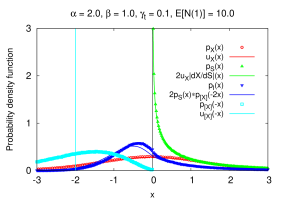
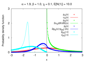
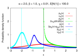
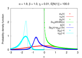
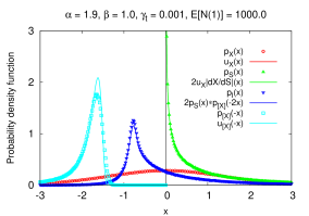
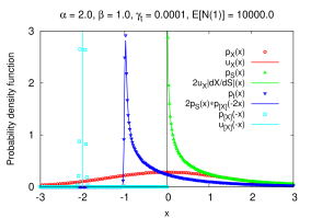
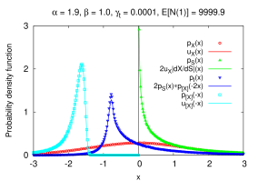
Figure 2: (Color online) Convergence of the empirical probability densities $p$ from 1 million Monte Carlo runs (points) to the analytic probability densities $u$ (lines) in the diffusive limit for a CTRW $X(t)$, its Stratonovich integral $S(t)$, its Itō integral $I(t)$, and its quadratic variation $[X](t)$, with $t=1$ and different choices of the index parameters $\alpha,\beta$ and of the scale parameters $\gamma_{x},\gamma_{t}$, where $\gamma_{x}^{\alpha}/\gamma_{t}^{\beta}=D=1$. $\mathbb{E}[N(t)]$ is the average number of jumps per run.

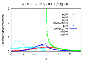
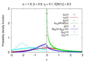
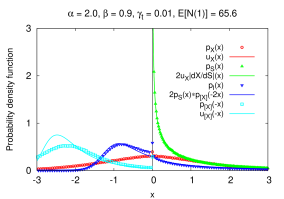
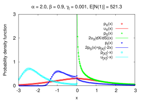
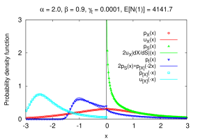
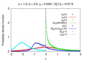
Figure 3: (Color online) Convergence of the empirical probability densities $p$ from 1 million Monte Carlo runs (points) to the analytic probability densities $u$ (lines) in the diffusive limit for a CTRW $X(t)$, its Stratonovich integral $S(t)$, its Itō integral $I(t)$, and its quadratic variation $[X](t)$, with $t=1$ and different choices of the index parameters $\alpha,\beta$ and of the scale parameters $\gamma_{x},\gamma_{t}$, where $\gamma_{x}^{\alpha}/\gamma_{t}^{\beta}=D=1$. $\mathbb{E}[N(t)]$ is the average number of jumps per run.

According to Eq. (37) here $I(t)=S(t)-[X](t)/2$; if the dependence of $S$ and $[X]$ is small, the probability density of the Itō integral is approximated by the convolution of the probability density of the Stratonovich integral with that of the quadratic variation mirrored around zero and scaled to half its width:

$$p_{I}(x,t)\simeq 2\int_{-\infty}^{+\infty}p_{S}(x+2x^{\prime},t)p_{[X]}(-2x^{\prime},t)\,dx^{\prime}.$$ (50)

For all choices of $\alpha$ and $\beta$ the agreement between the analytic expressions for $X(t)$ and $S(t)$ in the diffusive limit and the empirical results from Monte Carlo simulation of the CTRWs is fair already for the largest value $\gamma_{t}=0.1$: the curves cannot be distinguished by eye at the scale of our plots. Therefore we did not evaluate the analytic probability density for $X(t)$, Eq. (18), available for the particular case of a NCPP only, i.e. the left column of Fig. 2. Instead the quadratic variation $[X](t)$ and consequently the Itō integral tend visibly more slowly to their diffusive limits. For a NCPP the diffusive limit of $[X](t)$ is $[B](t)=2Dt$. In this limit $I(t)=S(t)-Dt=B^{2}(t)/2-Dt$, corresponding to the well-known result that the probability density of the Itō integral is equal to the density of the Stratonovich integral shifted by $-Dt$, i.e. $p_{I}(x,t)=p_{S}(x+Dt,t)$. Though the quadratic variation of the NCPP is appreciably different from its limit $\delta(x-2Dt)$, where $Dt=1$, for any non infinitesimal value of $\gamma_{t}$ as shown in the left column of Fig. 2, for $\gamma_{t}=0.01$ there is a good agreement between the Itō integrals from Monte Carlo and from Eq. (50).

The density of the quadratic variation for a CTRW can be obtained from the density of squared jumps, $\lambda_{\xi^{2}}(x)$, that results from a transformation of the density of jumps, $\lambda_{\xi}(\sqrt{x})$, similar to the one that leads from $p_{X}(x,t)$ to $p_{S}(x,t)$, Eq. (48), except for a factor 2:

$$\lambda_{\xi^{2}}(x;\gamma_{x})=\lambda_{\xi}(\sqrt{x};\gamma_{x})/\sqrt{x}$$ (51)

Inserting this equation into the solution of the Montroll-Weiss equation in the space-time domain, Eq. (16), gives

$$p_{[X]}(x,t;\gamma_{x},\gamma_{t})=\sum_{n=0}^{\infty}p_{N}(n,t;\gamma_{t})\lambda_{\xi^{2}}^{*n}(x;\gamma_{x}),$$ (52)

where $x>0$. Unfortunately even for an NCPP the $n$-fold convolution cannot be computed as easily as for $p_{X}(x,t)$ in Eq. (18). However, the characteristic function of the quadratic variation can be written as

$$\widehat{p}_{[X]}(k,t;\gamma_{x},\gamma_{t})=\sum_{n=0}^{\infty}p_{N}(n,t;\gamma_{t})\widehat{\lambda}_{\xi^{2}}^{n}(k;\gamma_{x}).$$ (53)

In order to consider non-exponential waiting times with power-law tails and infinite first moment, for the sake of simplicity let us assume that $p_{N}(n,t)$ is the distribution of the Mittag-Leffler counting process scalas04 ,

$$p_{N}(n,t;\gamma_{t})=\frac{(t/\gamma_{t})^{\beta n}}{n!}E_{\beta}^{(n)}\left(-(t/\gamma_{t})^{\beta}\right),$$ (54)

where

$$E_{\beta}^{(n)}(z)=\frac{d^{n}}{dz^{n}}E_{\beta}(z).$$ (55)

This choice is more general than it seems, as the Mittag-Leffler distribution for waiting times is an attractor for the thinning procedure used to obtain the diffusive limit mainardi04 . Using the Mittag-Leffler distribution from the beginning simplifies the derivation of this limit. Then Eq. (53) becomes scalas06

$$\widehat{\lambda}_{[X]}(k,t;\gamma_{x},\gamma_{t})=E_{\beta}\big{(}-(t/\gamma_{t})^{\beta}(1-\widehat{\lambda}_{\xi^{2}}(k;\gamma_{x}))\big{)}.$$ (56)

As the jumps $\xi$ follow a Lévy $\alpha$-stable distribution, for $x\rightarrow\infty,\ \lambda_{\xi^{2}}(x;\gamma_{x})\sim(x/\gamma_{x})^{-\alpha/2-1}$, and the sum of $\xi_{i}^{2}$ converges to the positive stable distribution with index $\alpha/2$, whose characteristic function is

$$\widehat{\lambda}_{\xi^{2}}(k;\gamma_{x})=\widehat{L}_{\alpha/2}^{+}(k;\gamma_{x})\equiv\exp\big{(}(-i\gamma_{x}^{2}k)^{\alpha/2}\big{)}.$$ (57)

The scale parameter $\gamma_{x}$ is the same as in the Lévy stable distribution, Eq. (20). Inserting this distribution in Eq. (56), the diffusive limit yields the following characteristic function for the quadratic variation:

$$\widehat{u}_{[X]}(k,t;D)=E_{\beta}\big{(}-D(-ik)^{\alpha/2}t^{\beta}\big{)}.$$ (58)

Now we can proceed in a similar fashion as for the solution of the FDE, Eqs. (29–30). Defining $\kappa=kt^{2\beta/\alpha}$ and

$$M_{\alpha,\beta}(\xi;D)=\mathcal{F}^{-1}_{\kappa}\big{[}E_{\beta}\big{(}-D(-i\kappa)^{\alpha/2}\big{)}\big{]}(\xi),$$ (59)

where $\quad\xi>0$, we obtain the quadratic variation for the diffusive limit in the space-time domain,

$$u_{[X]}(x,t;D)=t^{-2\beta/\alpha}\,M_{\alpha,\beta}(xt^{-2\beta/\alpha};D).$$ (60)

When $\alpha=2,\ M_{2,\beta}(\xi)$ coincides with the right half of the Mainardi-Wright function mainardi01 , which is also called M-function of Wright type because its shape recalls a capital M centered in the origin. When $\alpha=2$ and $\beta=1$ (standard diffusion case), a delta function $u_{[X]}(x,t;D)=\delta(x-2Dt)$ is recovered, corresponding to the quadratic variation of the Bachelier-Wiener process, $[X](t)=2Dt$. The plots in Figs. 2 and 3 display quadratic variations both from Monte Carlo and from Eq. (60). The convergence of the quadratic variation in the diffusive limit can be used to prove that the integrals of $X(t)$ as defined in Sec. II converge.

IV Conclusions and outlook

This paper is based on the definition, given in Eq. (II.1), of a class of stochastic integrals $J_{\vartheta}(t)$ driven by a CTRW $X(t)$. For $\vartheta=0$ this results in the Itō integral $I(t)$, Eq. (35), for $\vartheta=1/2$ in the Stratonovich integral. If the process $X(t)$ that defines the measure used in Eq. (35) is a martingale with respect to its natural filtration, then $I(t)$ is a martingale too; this is a consequence of the martingale transform theorem. It turns out that an uncoupled CTRW with zero-mean jumps is a martingale. The stochastic integration theory developed here is more general than the one sketched in Ref. zygadlo03 , as it can be applied also to a CTRW that is neither Markovian nor Lévy. In fact, exponential waiting times are not needed to prove that $I(t)$ is a martingale if $X(t)$ is a martingale.

The theory presented in Sec. II lies at the foundation of the Monte Carlo method for integrating stochastic differential equations driven by CTRWs. As explained in Sec. I, these results are relevant for applications in physics and economics as well as in all those fields like insurance and finance where martingale methods can help in the quantitative evaluation of risk. Eq. (II.1) is a convenient basis for the Monte Carlo calculation of stochastic integrals. This is shown in Sec. III, where Monte Carlo realizations of CTRWs are used to effectively approximate the Itō and Stratonovich integrals driven by the Bachelier-Wiener process and, more generally, by the solution of the space-time fractional diffusion equation.

We believe that up-to-date mathematical methods from probability theory and stochastic calculus are beneficial to the study of the CTRW and of other random processes useful in statistical physics. We fear that progress will be slower or impossible if these methods are ignored by physicists.

Future work will deal with Monte Carlo simulations for coupled CTRWs where jumps and waiting times obey fat-tailed distributions meerschaert02 ; meerschaert06 . There will also be a discussion of convergence based on the results collected in jacod03 .

Appendix

Below are salient lines from the central loop of our C++ program for the Monte Carlo calculation of a CTRW $X(t)$, its quadratic variation $[X(t)]$, its Itō integral $I(t)$ and its Stratonovich integral $S(t)$ as described in Sec. III and shown in Figs. 2–3.

jumps = 0

// Loop over runs
for (run = 1; run <= runs; run++) {

    // Initialize and increment t, x, etc.
    t = 0, x = 0, qvar = 0, ito = 0, str = 0,
    tau = random.t();          // Eq. (47)
    while (t + tau < t_max) {
        t += tau;              // time t
        xi = random.x();       // Eq. (46)
        qvar += xi*xi;         // [X(t)]
        ito += x*xi;           // I(t)
        str += (x+xi/2)*xi;    // S(t)
        x += xi;               // X(t)
        tau = random.t();      // Eq. (47)
        jumps++;               // N(t)
    }

    // Update histograms at the end of each run
    hisx.add(x);               // X(t)
    hisq.add(qvar);            // [X(t)]
    hisi.add(ito);             // I(t)
    hiss.add(str);             // S(t)
}

CPU times grow linearly with the number of jumps $N(t)$ and take 1–3 $\mu$sec per jump depending on $\alpha$ and $\beta$ on a 2.2 GHz AMD Athlon 64 X2 “Toledo” Dual-Core processor with Fedora Core 7 Linux, using the Ran uniform random number generator press07 and the GNU C++ compiler (g++) version 4.1.2 with the -O3 -static optimization options.

References

- (1) E. Montroll and G. H. Weiss, J. Math. Phys. 6, 167 (1965).
- (2) H. Scher and M. Lax, Phys. Rev. B 7, 4491 (1973).
- (3) H. Scher and M. Lax, Phys. Rev. B 7, 4502 (1973).
- (4) E. W. Montroll and H. Scher, J. Stat. Phys. 9, 101 (1973).
- (5) H. Scher and E. Montroll, Phys. Rev. B 12, 2455 (1975).
- (6) M. F. Shlesinger, Random processes, in Encyclopedia of Applied Physics, Vol. 16, edited by G. L. Trigg (VCH Publishers, New York, 1996), pp. 45–70.
- (7) G. H. Weiss, Aspects and Applications of the Random Walk (North-Holland, Amsterdam, 1994).
- (8) R. Metzler and J. Klafter, Phys. Rep. 339, 1 (2000).
- (9) R. Metzler and J. Klafter, J. Phys. A: Math. Gen. 37, R161 (2004).
- (10) D. Fulger, E. Scalas, and G. Germano, Phys. Rev. E 77, 021122 (2008).
- (11) M. M. Meerschaert and H. P. Scheffler, Limit Distributions for Sums of Independent Random Vectors: Heavy Tails in Theory and Practice (Wiley, New York, 2001).
- (12) D. R. Cox, Renewal Theory (Methuen, London, 1967).
- (13) W. Feller, An Introduction to Probability Theory and its Applications, Vol. 2 (Wiley, New York, 1971).
- (14) D. R. Cox and V. Isham, Point Processes (Chapman & Hall, London, 1979).
- (15) P. Billingsley, Probability and Measure (Wiley, New York, 1979).
- (16) P. G. Hoel, S. C. Port, and J. Stone, Introduction to Stochastic Processes (Houghton Mifflin, Boston, 1972).
- (17) E. Çinlar, Introduction to Stochastic Processes (Prentice-Hall, Englewood Cliffs, 1975).
- (18) O. Flomenbom, J. Klafter, Phys. Rev. Lett. 95, 098105 (2005).
- (19) O. Flomenbom, R. J. Silbey, Phys. Rev. E 76, 041101 (2007).
- (20) J. Janssen and R. Manca, Semi-Markov Risk Models for Finance, Insurance and Reliability (Springer, New York, 2007).
- (21) J. Bertoin, Lévy Processes (Cambridge University Press, Cambridge, UK, 1996).
- (22) K.-I. Sato, Lévy Processes and Infinitely Divisible Distributions (Cambridge University Press, Cambridge, UK, 1999).
- (23) M. F. Shlesinger, J. Stat. Phys. 10, 421 (1974).
- (24) J. K. E. Tunaley, J. Stat. Phys. 11, 397 (1974).
- (25) J. K. E. Tunaley, J. Stat. Phys. 12, 1 (1975).
- (26) J. K. E. Tunaley, J. Stat. Phys. 14, 461 (1976).
- (27) M. F. Shlesinger, J. Klafter, and Y. M. Wong, J. Stat. Phys. 27, 499 (1982).
- (28) D. ben-Avraham and S. Havlin, Diffusion and Reactions in Fractals and Disordered Systems (Cambridge University Press, Cambridge, UK, 2000).
- (29) V. Balakrishnan, Physica A 132, 569 (1985).
- (30) R. Hilfer and L. Anton, Phys. Rev. E 51, R848 (1995).
- (31) E. Scalas, R. Gorenflo, and F. Mainardi, Phys. Rev. E 69, 011107 (2004).
- (32) E. Scalas, Physica A 362, 225 (2006).
- (33) D. del-Castillo-Negrete, B. A. Carreras, and V. E. Lynch, Phys. Rev. Lett. 94, 065003 (2005).
- (34) J. L. A. Dubbeldam, A. Milchev, V. G. Rostiashvili, and T. A. Vilgis, Phys. Rev. E 76, 010801 (2007).
- (35) J. L. A. Dubbeldam, A. Milchev, V. G. Rostiashvili, and T. A. Vilgis, Europhys. Lett. 79, 18002 (2007).
- (36) J. Masoliver, M. Montero, J. Perelló, and G. H. Weiss, J. Econ. Behav. Organ. 61, 577 (2006).
- (37) P. Embrechts, C. Klüppelberg, and T. Mikosch, Modelling Extremal Events for Insurance and Finance (Springer, New York, 1997).
- (38) Á. Cartea and D. del-Castillo-Negrete, Phys. Rev. E 76, 041105 (2007).
- (39) R. Zygadło, Phys. Rev. E, 68, 046117 (2003).
- (40) R. C. Merton, J. Financ. Econ. 3, 125 (1976).
- (41) R. Gorenflo, J. Loutchko, Yu Luchko, Fract. Calc. Appl. Anal. 5, 491 (2002).
- (42) I. Polubny and Martin Kacenak, mlf.m: Mittag-Leffler function — Calculates the Mittag-Leffler function with desired accuracy, MATLAB Central File Exchange, file ID #8738 (2005), www.mathworks.com/matlabcentral/fileexchange.
- (43) R. Hilfer and H. J. Seybold, Integr. Transf. Spec. F., 17, 637, (2006).
- (44) S. G. Samko, A. A. Kilbas, and O. Marichev, Fractional Integrals and Derivatives, Theory and Applications (Gordon and Breach Science Publishers, London, 1993).
- (45) I. Podlubny, Fractional Differential Equations (Academic Press, San Diego, 1999).
- (46) R. Metzler, J. Klafter, and I. Sokolov, Phys. Rev. E 58, 1621 (1999).
- (47) R. Metzler, E. Barkai, and J. Klafter, Phys. Rev. Lett. 82, 3563 (1999).
- (48) R. Metzler, E. Barkai, and J. Klafter, Europhys. Lett. 46, 431 (1999).
- (49) E. Barkai, R. Metzler, and J. Klafter, Phys. Rev. E 61, 132 (2000).
- (50) M. Magdziarz, A. Weron, and K. Weron, Phys. Rev. E 75, 016708 (2007).
- (51) N. G. van Kampen, Stochastic Processes in Physics and Chemistry (North-Holland, Amsterdam, 1981).
- (52) H. Risken, The Fokker-Planck Equation. Methods of Solution and Applications, 2nd edition with corrections (Springer, Berlin, 1992).
- (53) F. Mainardi, M. Raberto, R. Gorenflo, and E. Scalas, Physica A 287, 468 (2000).
- (54) A. Mura, M. S. Taqqu, and F. Mainardi, Physica A 387, 5033 (2008).
- (55) I. M. Gel’fand and G. E. Shilov, Generalized Functions (Academic Press, New York, 1964).
- (56) P. Protter, Stochastic Integration and Differential Equations, 2nd edition (Springer, Berlin, 2004).
- (57) W. Paul and J. Baschnagel, Stochastic Processes — From Physics to Finance (Springer, Berlin, 2000).
- (58) C. W. Gardiner, Handbook of Stochastic Methods, 2nd edition, (Springer, Berlin, 1996).
- (59) D. Williams, Probability with Martingales (Cambridge University Press, Cambridge, UK, 1991).
- (60) R. L. Schilling, Measures, Integrals and Martingales (Cambridge University Press, Cambridge, UK, 2005).
- (61) L. Devroye, Non-Uniform Random Variate Generation (Springer, New York, 1986).
- (62) L. Devroye, in Proceedings of the 1996 Winter Simulation Conference, edited by J. M. Charnes, D. J. Morrice, D. T. Brunner, and J. J. Swain (IEEE Press, New York, 1996), pp. 265–272.
- (63) J. M. Chambers, C. L. Mallows, and B. W. Stuck, J. Am. Stat. Assoc. 71, 340 (1999).
- (64) J. H. McCulloch, stabrnd.m: Stable random number generator, Matlab script (1996), www.econ.ohio-state.edu/jhm/jhm.html.
- (65) T. J. Kozubowski and S. T. Rachev, Int. J. Comput. Numer. Anal. Appl. 1, 177 (1999).
- (66) G. Germano, D. Fulger, and E. Scalas, mlrnd.m: Mittag-Leffler pseudo-random number generator, Matlab Central File Exchange, file ID #19392 (2008).
- (67) F. Mainardi, R. Gorenflo and E. Scalas, Vietnam J. Math. 32, 53 (2004).
- (68) F. Mainardi, Yu. Luchko and G. Pagnini, Fract. Calc. Appl. Anal. 4, 153 (2001).
- (69) M. M. Meerschaert, D. A. Benson, H.-P. Scheffler, P. Becker-Kern, Phys. Rev. E 66, 060102 (2002).
- (70) M. M. Meerschaert and E. Scalas, Physica A 370, 114 (2006).
- (71) J. Jacod and A. N. Shiryaev, Limit Theorems for Stochastic Processes, 2nd edition, Vol. 288 of Grundlehren der mathematischen Wissenschaften (Springer, Berlin, 2003).
- (72) W. H. Press, Saul A. Teukolsky, William T. Vetterling, Brian P. Flannery, Numerical Recipes — The Art of Scientific Computing, 3rd edition (Cambridge University Press, Cambridge, UK, 2007).