Asymptotically optimal quantization schemes for Gaussian processes

Abstract

We describe quantization designs which lead to asymptotically and order optimal functional quantizers. Regular variation of the eigenvalues of the covariance operator plays a crucial role to achieve these rates. For the development of a constructive quantization scheme we rely on the knowledge of the eigenvectors of the covariance operator in order to transform the problem into a finite dimensional quantization problem of normal distributions.

Keywords: Functional quantization, Gaussian process, Brownian Motion, Riemann-Liouville process, optimal quantizer.

MSC: 60G15, 60E99.

1 Introduction

Functional quantization of stochastic processes can be seen as a discretization of the path-space of a process and the approximation (coding) of a process by finitely many deterministic functions from its path-space. In a Hilbert space setting this reads as follows.

Let $(H,<\cdot,\cdot>)$ be a separable Hilbert space with norm $\|\cdot\|$ and let $X:(\Omega,{\cal A},{P})\rightarrow H$ be a random vector taking its values in $H$ with distribution ${P}_{X}$. For $n\in{N}$, the $L^{2}$-quantization problem for $X$ of level $n$ (or of nat-level $\log n$) consists in minimizing

$$\left({E}\min_{a\in\alpha}\|X-a\|^{2}\right)^{1/2}=\|\min_{a\in\alpha}\|X-a\|\|_{L^{2}({P})}$$

over all subsets $\alpha\subset H$ with $\mbox{card}(\alpha)\leq n$. Such a set $\alpha$ is called $n$-codebook or $n$-quantizer. The minimal $n$th quantization error of $X$ is then defined by

$$e_{n}(X):=\inf\left\{({E}\min_{a\in\alpha}\|X-a\|^{2})^{1/2}:\alpha\subset H,\;\mbox{card}(\alpha)\leq n\right\}.$$ (1.1)

Under the integrability condition

$${E}\,\|X\|^{2}<\infty$$ (1.2)

the quantity $e_{n}(X)$ is finite.

For a given $n$-quantizer $\alpha$ one defines an associated closest neighbour projection

$$\pi_{\alpha}:=\sum\limits_{a\in\alpha}a\mbox{\bf 1}_{C_{a}(\alpha)}$$

and the induced $\alpha$-quantization (Voronoi quantization) of $X$ by

$$\hat{X}^{\alpha}:=\pi_{\alpha}(X),$$ (1.3)

where $\{C_{a}(\alpha):a\in\alpha\}$ is a Voronoi partition induced by $\alpha$, that is a Borel partition of $H$ satisfying

$$C_{a}(\alpha)\subset V_{a}(\alpha):=\{x\in H:\|x-a\|=\min_{b\in\alpha}\|x-b\|\}$$ (1.4)

for every $a\in\alpha$. Then one easily checks that, for any random vector $X^{{}^{\prime}}:\Omega\rightarrow\alpha\subset H$,

$${E}\,\|X-X^{{}^{\prime}}\|^{2}\geq\,{E}\,\|X-\hat{X}^{\alpha}\|^{2}={E}\,\min_{a\in\alpha}\|X-a\|^{2}$$

so that finally

$$e_{n}(X) = \inf\left\{({E}\,\|X-\hat{X}\|^{2})^{1/2}:\hat{X}=f(X),f:H\rightarrow H\;\mbox{Borel measurable,}\;\right.$$

$$\left.\qquad\mbox{card}(f(H))\leq n\right\}$$

$$= \inf\left\{({E}\,\|X-\hat{X}\|^{2})^{1/2}:\hat{X}:\Omega\rightarrow H\;\mbox{random vector,}\;\mbox{card}(\hat{X}(\Omega))\leq n\right\}.$$

Observe that the Voronoi cells $V_{a}(\alpha),a\in\alpha$ are closed and convex (where convexity is a characteristic feature of the underlying Hilbert structure). Note further that there are infinitely many $\alpha$-quantizations of $X$ which all produce the same quantization error and $\hat{X}^{\alpha}$ is ${P}$-a.s. uniquely defined if ${P}_{X}$ vanishes on hyperplanes.

A typical setting for functional quantization is $H=L^{2}([0,1],dt)$ but is obviously not restricted to the Hilbert space setting. Functional quantization is the natural extension to stochastic processes of the so-called optimal vector quantization of random vectors in $H={R}^{d}$ which has been extensively investigated since the late 1940’s in Signal processing and Information Theory (see [4], [7]). For the mathematical aspects of vector quantization in ${R}^{d}$, one may consult [5], for algorithmic aspects see [16] and ”non-classical” applications can be found in [14], [15]. For a first promising application of functional quantization to the pricing of financial derivatives through numerical integration on path-spaces see [17].

We address the issue of high-resolution quantization which concerns the performance of $n$-quantizers and the behaviour of $e_{n}(X)$ as $n\rightarrow\infty$. The asymptotics of $e_{n}(X)$ for ${R}^{d}$-valued random vectors has been completely elucidated for non-singular distributions ${P}_{X}$ by the Zador Theorem (see [5]) and for a class of self-similar (singular) distributions by [6]. In infinite dimensions no such global results hold, even for Gaussian processes.

It is convenient to use the symbols $\sim$ and $\stackrel{{\scriptstyle<}}{{\sim}}$, where $a_{n}\sim b_{n}$ means $a_{n}/b_{n}\rightarrow 1$ and $a_{n}\stackrel{{\scriptstyle<}}{{\sim}}b_{n}$ means $\limsup_{n\to\infty}a_{n}/b_{n}\leq 1$. A measurable function $\varphi:(s,\infty)\rightarrow(0,\infty)\,(s\geq 0)$ is said to be regularly varying at infinity with index $b\in{R}$ if, for every $c>0$,

$$\lim_{x\to\infty}\frac{\varphi(cx)}{\varphi(x)}=c^{b}.$$

Now let $X$ be centered Gaussian. Denote by $K_{X}\subset H$ the reproducing kernel Hilbert space (Cameron-Martin space) associated to the covariance operator

$$C_{{}_{X}}:H\rightarrow H,\;C_{{}_{X}}y:={E}\,(<\!y,X\!>\!X)$$ (1.6)

of $X$. Let $\lambda_{1}\geq\lambda_{2}\geq\ldots>0$ be the ordered nonzero eigenvalues of $C_{{}_{X}}$ and let $\{u_{j}:j\geq 1\}$ be the corresponding orthonormal basis of supp$({P}_{X})$ consisting of eigenvectors (Karhunen-Loève basis). If $d:=\dim K_{X}<\infty$, then $e_{n}(X)=e_{n}\left(\bigotimes\limits^{d}_{j=1}\mathcal{N}(0,\lambda_{j})\right)$, the minimal $n$th $L^{2}$-quantization error of $\bigotimes\limits^{d}_{j=1}\mathcal{N}(0,\lambda_{j})$ with respect to the $l_{2}$-norm on ${R}^{d}$, and thus we can read off the asymptotic behaviour of $e_{n}(X)$ from the high-resolution formula

$$e_{n}(\bigotimes\limits^{d}_{j=1}\mathcal{N}(0,\lambda_{j}))\sim q(d)\sqrt{2\pi}\left(\Pi^{d}_{j=1}\lambda_{j}\right)^{1/2d}\left(\frac{d+2}{d}\right)^{(d+2)/4}n^{-1/d}\;\mbox{ as }\;n\rightarrow\infty$$ (1.7)

where $q(d)\in(0,\infty)$ is a constant depending only on the dimension $d$ (see [5]). Except in dimension $d=1$ and $d=2$, the true value of $q(d)$ is unknown. However, one knows (see [5]) that

$$q(d)\sim\left(\frac{d}{2\pi e}\right)^{1/2}\;\mbox{ as }\;d\rightarrow\infty.$$ (1.8)

Assume $\dim K_{X}=\infty$. Under regular behaviour of the eigenvalues the sharp asymptotics of $e_{n}(X)$ can be derived analogously to (1.7). In view of (1.8) it is reasonable to expect that the limiting constants can be evaluated. The recent high-resolution formula is as follows.

Theorem 1.

([11]) Let $X$ be a centered Gaussian. Assume $\lambda_{j}\sim\varphi(j)$ as $j\rightarrow\infty$, where $\varphi:(s,\infty)\rightarrow(0,\infty)$ is a decreasing, regularly varying function at infinity of index $-b<-1$ for some $s\geq 0$. Set, for every $x>s$,

$$\psi(x):=\frac{1}{x\varphi(x)}.$$

Then

$$e_{n}(X)\sim\left(\left(\frac{b}{2}\right)^{b-1}\!\!\frac{b}{b-1}\right)^{1/2}\psi(\log n)^{-1/2}\;\mbox{ as }\;\vspace{0.5cm}n\rightarrow\infty.$$

A high-resolution formula in case $b=1$ is also available (see [11]). Note that the restriction $-b\leq-1$ on the index of $\varphi$ is natural since $\sum\limits^{\infty}_{j=1}\lambda_{j}<\infty$. The minimal $L^{r}$-quantization errors of $X$, $0<r<\infty$, are strongly equivalent to the $L^{2}$-errors $e_{n}(X)$ (see [3]) and thus exhibit the same high-resolution behaviour.

The paper is organized as follows. In Section 2 we investigate a quantization design, which furnishes asymptotically optimal quantizers in the situation of Theorem 1. Here the Karhunen-Loève expansion plays a crucial role. In section 3 we state different quantization designs, which are all at least order-optimal and discuss their possible implementations regarding the example of the Brownian motion. The main focus in that section lies on ”good” designs for finite $n\in{N}$.

2 Asymptotically optimal functional quantizers

Let $X$ be a $H$-valued random vector satisfying (1.2). For every $n\in{N}$, $L^{2}$-optimal $n$-quantizers $\alpha\subset H$ exist, that is

$$({E}\,\min_{a\in\alpha}\|X-a\|^{2})^{1/2}=e_{n}(X).$$

If card (supp$({P}_{X}))\geq n$, optimal $n$-quantizers $\alpha$ satisfy card$(\alpha)=n$, ${P}(X\in C_{a}(\alpha))>0$ and the stationarity condition

$$a={E}\,(X\mid\{X\in C_{a}(\alpha)\}),\,a\in\alpha$$ (2.1)

or what is the same

$$\hat{X}^{\alpha}={E}\,(X\mid\hat{X}^{\alpha})$$ (2.2)

for every Voronoi partition $\{C_{a}(\alpha):a\in\alpha\}$ (see [10]). In particular, ${E}\,\hat{X}^{\alpha}={E}\,X$.

Now let $X$ be centered Gaussian with $\dim K_{X}=\infty$. The Karhunen-Loève basis $\{u_{j}:j\geq 1\}$ consisting of normalized eigenvectors of $C_{{}_{X}}$ is optimal for the quantization of Gaussian random vectors (see [10]). So we start with the Karhunen-Loève expansion

$$X\stackrel{{\scriptstyle H}}{{=}}\sum\limits^{\infty}_{j=1}\lambda^{1/2}_{j}\xi_{j}u_{j},$$

where $\xi_{j}=<\!X,u_{j}\!>/\lambda^{1/2}_{j},j\geq 1$ are i.i.d. $\mathcal{N}(0,1)$-distributed random variables. The design of an asymptotically optimal quantization of $X$ is based on optimal quantizing blocks of coefficients of variable ($n$-dependent) block length. Let $n\in{N}$ and fix temporarily $m,l,n_{1},\ldots,n_{m}\in{N}$ with $\Pi^{m}_{j=1}n_{j}\leq n$, where $m$ denotes the number of blocks, $l$ the block length and $n_{j}$ the size of the quantizer for the $j$th block

$$\xi^{(j)}:=(\xi_{(j-1)l+1},\ldots,\xi_{jl}),\quad j\in\{1,\ldots,m\}.$$

Let $\alpha_{j}\subset{R}^{l}$ be an $L^{2}$-optimal $n_{j}$-quantizer for $\xi^{(j)}$ and let $\widehat{\xi^{(j)}}=\widehat{\xi^{(j)}}^{\alpha_{j}}$ be a $\alpha_{j}$-quantization of $\xi^{(j)}$. (Quantization of blocks $\xi^{(j)}$ instead of $(\lambda^{1/2}_{(j-1)l+1}\xi_{(j-1)l+1},\ldots,\lambda^{1/2}_{jl}\xi_{jl})$ is asymptotically good enough. For finite $n$ the quantization scheme will be considerably improved in Section 3. ) Then, define a quantized version of $X$ by

$$\hat{X}^{n}:=\sum\limits^{m}_{j=1}\sum\limits^{l}_{k=1}\lambda^{1/2}_{(j-1)l+k}(\widehat{\xi^{(j)}})_{k}u_{(j-1)l+k}.$$ (2.3)

It is clear that card$(\hat{X}^{n}(\Omega))\leq n$. Using (2.2) for $\xi^{(j)}$, one gets ${E}\,\hat{X}^{n}=0$. If

$$\widehat{\xi^{(j)}}=\sum\limits_{b\in\alpha_{j}}b\mbox{\bf 1}_{C_{b}(\alpha_{j})}(\xi^{(j)}),$$

then

$$\hat{X}^{n}=\sum\limits_{a\in\times^{m}_{j=1}\alpha_{j}}(\sum\limits^{m}_{j=1}\sum\limits^{l}_{k=1}\lambda^{1/2}_{(j-1)l+k}a^{(j)}_{k}u_{(j-1)l+k})\Pi^{m}_{j=1}\mbox{\bf 1}_{C_{a^{(j)}}(\alpha_{j})}(\xi^{(j)})$$

where $a=(a^{(1)},\ldots,a^{(m)})\in\times^{m}_{j=1}\alpha_{j}$. Observe that in general, $\hat{X}^{n}$ is not a Voronoi quantization of $X$ since it is based on the (less complicated) Voronoi partitions for $\xi^{(j)},j\leq m$. $(\hat{X}^{n}$ is a Voronoi quantization if $l=1$ or if $\lambda_{(j-1)l+1}=\ldots=\lambda_{jl}$ for every $j$.) Using again (2.2) for $\xi^{(j)}$ and the independence structure, one checks that $\hat{X}^{n}$ satisfies a kind of stationarity equation:

$${E}\,(X\mid\hat{X}^{n})=\hat{X}^{n}.$$

Lemma 1.

Let $n\geq 1$. For every $l\geq 1$ and every $m\geq 1$

$${E}\,\|X-\hat{X}^{n}\|^{2}\leq\sum\limits^{m}_{j=1}\lambda_{(j-1)l+1}e_{n_{j}}(N(0,I_{l}))^{2}+\sum\limits_{j\geq ml+1}\lambda_{j}.$$ (2.4)

Furthermore, (2.4) stands as an equality if $l=1$ (or $\lambda_{(j-1)l+1}=\ldots=\lambda_{jl}$ for every $j,\,l\geq 1$).

Proof. The claim follows from the orthonormality of the basis $\{u_{j}:j\geq 1\}$. We have

$$\begin{array}[]{lcl}{E}\,\|X-\hat{X}^{n}\|^{2}&=&\sum\limits^{m}_{j=1}\sum\limits^{l}_{k=1}\lambda_{(j-1)l+k}{E}\,\mid\xi^{(j)}_{k}-(\widehat{\xi^{(j)}})_{k}\mid^{2}+\sum\limits_{j\geq ml+1}\lambda_{j}\\ &\leq&\sum\limits^{m}_{j=1}\lambda_{(j-1)l+1}\sum\limits^{l}_{k=1}{E}\,\mid\xi^{(j)}_{k}-\widehat{\xi^{(j)}})_{k}\mid^{2}+\sum\limits_{j\geq ml+1}\lambda_{j}\\ &=&\sum\limits^{m}_{j=1}\lambda_{(j-1)l+1}e_{n_{j}}(\xi^{(j)})^{2}+\sum\limits_{j\geq ml+1}\lambda_{j}.\end{array}$$

$\Box$

Set

$$C(l):=\sup_{k\geq 1}k^{2/l}e_{k}(N(0,I_{l}))^{2}.$$ (2.5)

By (1.7), $C(l)<\infty$. For every $l\in{N}$,

$$e_{n_{j}}(N(0,I_{l})^{2}\leq n^{-2/l}_{j}C(l)$$ (2.6)

Then one may replace the optimization problem which consists, for fixed $n$, in minimizing the right hand side of Lemma 1 by the following optimal allocation problem:

$$\min\{C(l)\sum\limits^{m}_{j=1}\lambda_{(j-1)l+1}n^{-2/l}_{j}+\sum\limits_{j\geq ml+1}\lambda_{j}:m,l,n_{1},\ldots,n_{m}\in{N},\Pi^{m}_{j=1}n_{j}\leq n\}.$$ (2.7)

Set

$$m=m(n,l):=\max\{k\geq 1:n^{1/k}\lambda_{(k-1)l+1}^{l/2}(\Pi^{k}_{j=1}\lambda_{(j-1)l+1})^{-l/2k}\geq 1\},$$ (2.8)

$$n_{j}=n_{j}(n,l):=[n^{1/m}\lambda^{l/2}_{(j-1)l+1}(\Pi^{m}_{i=1}\lambda_{(i-1)l+1})^{-l/2m}],\;j\in\{1,\ldots,m\},$$ (2.9)

where $[x]$ denotes the integer part of $x\in{R}$ and

$$l=l_{n}:=[(\max\{1,\log n\})^{\vartheta}],\;\vartheta\in(0,1).$$ (2.10)

In the following theorem it is demonstrated that this choice is at least asymptotically optimal provided the eigenvalues are regularly varying.

Theorem 2.

Assume the situation of Theorem 1. Consider $\hat{X}^{n}$ with tuning parameters defined in (2.8)-(2.10). Then $\hat{X}^{n}$ is asymptotically $n$-optimal, i.e.

$$({E}\,\|X-\hat{X}^{n}\|^{2})^{1/2}\sim e_{n}(X)\;\mbox{ as }\;n\rightarrow\infty.$$

Note that no block quantizer with fixed block length is asymptotically optimal (see [11]). As mentioned above, $\hat{X}^{n}$ is not a Voronoi quantization of $X$. If $\alpha_{n}:=\hat{X}^{n}(\Omega)$, then the Voronoi quantization $\hat{X}^{\alpha_{n}}$ is clearly also asymptotically $n$-optimal.

The key property for the proof is the following $l$-asymptotics of the constants $C(l)$ defined in (2.5). It is interesting to consider also the smaller constants

$$Q(l):=\lim_{k\to\infty}k^{2/l}e_{k}(\mathcal{N}(0,I_{l}))^{2}$$ (2.11)

(see (1.7)).

Proposition 1.

The sequences $(C(l))_{l\geq 1}$ and $(Q(l))_{l\geq 1}$ satisfy

$$\lim_{l\to\infty}\frac{C(l)}{l}=\lim_{l\to\infty}\frac{Q(l)}{l}=\inf_{l\geq 1}\frac{C(l)}{l}=\inf_{l\geq 1}\frac{Q(l)}{l}=1.$$

Proof. From [11] it is known that

$$\liminf_{l\to\infty}\frac{C(l)}{l}=1.$$ (2.12)

Furthermore, it follows immediately from (1.7) and (1.8) that

$$\lim_{l\to\infty}\frac{Q(l)}{l}=1.$$ (2.13)

(The proof of the existence of $\displaystyle\lim_{l\to\infty}C(l)/l$ we owe to S. Dereich.) For $l_{0},l\in{N}$ with $l\geq l_{0}$, write

$$l=n\,l_{0}+m\;\mbox{with}\;n\in{N},m\in\{0,\ldots,l_{0}-1\}.$$

Since for every $k\in{N}$,

$$[k^{l_{0}/l}]^{n}\;[k^{1/l}]^{m}\leq k,$$

one obtains by a block-quantizer design consisting of $n$ blocks of length $l_{0}$ and $m$ blocks of length 1 for quantizing $N(0,I_{l})$,

$$e_{k}(\mathcal{N}(0,I_{l}))^{2}\leq ne_{[k^{l_{0}/l}]}(\mathcal{N}(0,I_{l_{0}}))^{2}+me_{[k^{1/l}]}(\mathcal{N}(0,1))^{2}.$$ (2.14)

This implies

$$C(l) \leq nC(l_{0})\sup_{k\geq 1}\frac{k^{2/l}}{[k^{l_{0}/l}]^{2/l_{0}}}+mC(1)\sup_{k\geq 1}\frac{k^{2/l}}{[k^{1/l}]^{2}}$$

$$\leq 4^{1/l_{0}}nC(l_{0})+4mC(1).$$

Consequently, using $n/l\leq 1/l_{0}$,

$$\frac{C(l)}{l}\leq\frac{4^{1/l_{0}}C(l_{0})}{l_{0}}+\frac{4mC(1)}{l}$$

and hence

$$\limsup_{l\to\infty}\frac{C(l)}{l}\leq\frac{4^{1/l_{0}}C(l_{0})}{l_{0}}.$$

This yields

$$\limsup_{l\to\infty}\frac{C(l)}{l}\leq\liminf_{l_{0}\rightarrow\infty}\frac{C(l_{0})}{l_{0}}=1.$$ (2.15)

It follows from (2.14) that

$$Q(l)\leq nQ(l_{0})+mQ(1).$$

Consequently

$$\frac{Q(l)}{l}\leq\frac{Q(l_{0})}{l_{0}}+\frac{mQ(1)}{l}$$

and therefore

$$1=\lim_{l\to\infty}\frac{Q(l)}{l}\leq\frac{Q(l_{0})}{l_{0}}.$$

This implies

$$\inf_{l_{0}\geq 1}\frac{Q(l_{0})}{l_{0}}=1.$$ (2.16)

Since $Q(l)\leq C(l)$, the proof is complete. $\Box$

The $n$-asymptotics of the number $m(n,l_{n})l_{n}$ of quantized coefficients in the Karhunen-Loève expansion in the quantization $\hat{X}^{n}$ is as follows.

Lemma 2.

([12], Lemma 4.8) Assume the situation of Theorem 1. Let $m(n,l_{n})$ be defined by (2.8) and (2.10). Then

$$m(n,l_{n})l_{n}\sim\frac{2\log n}{b}\;\mbox{ as }\;n\rightarrow\infty.$$

Proof of Theorem 2. For every $n\in{N}$,

$$\sum\limits^{m}_{j=1}\lambda_{(j-1)l+1}n^{-2/l}_{j} \leq \sum\limits^{m}_{j=1}\lambda_{(j-1)l+1}(n_{j}+1)^{-2/l}(\frac{n_{j}+1}{n_{j}})^{2/l}$$

$$\leq 4^{1/l}mn^{-2/ml}(\Pi^{m}_{j=1}\lambda_{(j-1)l+1})^{1/m}$$

$$\leq 4^{1/l}m\lambda_{(m-1)l+1}.$$

Therefore, by Lemma 1 and (2.6),

$${E}\,\|X-\hat{X}^{n}\|^{2}\leq 4^{1/l}\frac{C(l)}{l}ml\lambda_{(m-1)l+1}+\sum\limits_{j\geq ml+1}\lambda_{j}$$

for every $n\in{N}$. By Lemma 2, we have

$$ml=m(n,l_{n})l_{n}\sim\frac{2\log n}{b}\;\mbox{ as }\;n\rightarrow\infty.$$

Consequently, using regular variation at infinity with index $-b<-1$ of the function $\varphi$,

$$ml\lambda_{(m-1)l+1}\sim ml\lambda_{ml}\sim\left(\frac{2}{b}\right)^{1-b}\psi(\log n)^{-1}$$

and

$$\sum\limits_{j\geq ml+1}\lambda_{j}\sim\frac{ml\varphi(ml)}{b-1}\sim\frac{1}{b-1}\left(\frac{2}{b}\right)^{1-b}\psi(\log n)^{-1}\;\mbox{ as }\;n\rightarrow\infty,$$

where, like in Theorem 1, $\psi(x)=1/x\varphi(x)$. Since by Proposition 1,

$$\lim_{n\to\infty}\frac{4^{1/l_{n}}C(l_{n})}{l_{n}}=1,$$

one concludes

$${E}\,\|X-\hat{X}^{n}\|^{2}\stackrel{{\scriptstyle<}}{{\sim}}\left(\frac{2}{b}\right)^{1-b}\frac{b}{b-1}\,\psi(\log n)^{-1}\;\mbox{ as }\;n\rightarrow\infty.$$

The assertion follows from Theorem 1. $\Box$

Let us briefly comment on the true dimension of the problem.

For $n\in{N}$, let ${\cal C}_{n}(X)$ be the (nonempty) set of all $L^{2}$-optimal $n$-quantizers. We introduce the integral number

$$d_{n}^{\ast}(X):=\min\left\{\mbox{dim}\;\mbox{span}\;(\alpha):\alpha\in{\cal C}_{n}(X)\right\}.$$ (2.17)

It represents the dimension at level $n$ of the functional quantization problem for $X$. Here span$(\alpha)$ denotes the linear subspace of $H$ spanned by $\alpha$. In view of Lemma 2, a reasonable conjecture for Gaussian random vectors is $d_{n}^{\ast}(X)\sim 2\log n/b$ in regular cases, where $-b$ is the regularity index. We have at least the following lower estimate in the Gaussian case.

Proposition 2.

Assume the situation of Theorem 1. Then

$$d_{n}^{\ast}(X)\stackrel{{\scriptstyle>}}{{\sim}}\frac{1}{b^{1/(b-1)}}\;\frac{2\log n}{b}\;\mbox{ as }\;n\rightarrow\infty.\vspace{0.5cm}$$

Proof. For every $n\in{N}$, we have

$$d_{n}^{\ast}(X)=\min\left\{k\geq 0:e_{n}(\bigotimes^{k}_{j=1}N(0,\lambda_{j}))^{2}+\sum\limits_{j\geq k+1}\lambda_{j}\leq e_{n}(X)^{2}\right\}$$ (2.18)

(see [10]). Define

$$c_{n}:=\min\left\{k\geq 0:\sum\limits_{j\geq k+1}\lambda_{j}\leq e_{n}(X)^{2}\right\}.$$

Clearly, $c_{n}$ increases to infinity as $n\rightarrow\infty$ and by (2.18), $c_{n}\leq d_{n}^{\ast}(X)$ for every $n\in{N}$. Using Theorem 1 and the fact that $\psi$ is regularly varying at infinity with index $b-1$, we obtain

$$((b-1)\psi(c_{n}))^{-1}\sim\sum\limits_{j\geq c_{n}+1}\lambda_{j}\sim e_{n}(X)^{2}\sim\left(\frac{2}{b}\right)^{1-b}\frac{b}{b-1}\,\psi(\log n)^{-1}$$

and thus

$$\psi(c_{n})\sim\left(\frac{2}{b}\right)^{1-b}\frac{1}{b}\psi(\log n)\sim\psi\left(\frac{1}{b^{1/(b-1)}}\;\frac{2\log n}{b}\right)\;\mbox{ as }\;n\rightarrow\infty.$$

Consequently,

$$c_{n}\sim\frac{1}{b^{1/(b-1)}}\;\frac{2\log n}{b}\;\mbox{ as }\;n\rightarrow\infty.$$

This yields the assertion. $\Box$

3 Quantizer designs and applications

In this section we are no longer interested in only asymptotically optimal quantizers of a Gaussian process $X$, but rather in really optimal or at least locally optimal quantizers for finite $n\in{N}$.

As soon as the Karhunen-Loève basis $(u_{j})_{j\geq 1}$ and the corresponding eigenvalues $(\lambda_{j})_{j\geq 1}$ of the Gaussian process $X$ are known, it is possible to transform the quantization problem of $X$ in $H$ into the quantization of $\bigotimes_{j=1}^{\infty}\mathcal{N}(0,\lambda_{j})$ on $l^{2}$ by the isometry $S:H\rightarrow l^{2}$

$$x\mapsto\left(<u_{j},x>\right)_{j\geq 1}.$$

and its inverse

$$S^{-1}:(l^{2},<\cdot\;,\cdot>_{K})\rightarrow(H,<\cdot,\cdot>),\quad l\mapsto\sum_{j\geq 1}l_{j}u_{j}.$$ (3.1)

The transformed problem then allows as we will see later on a direct access by vector quantization methods.

The following result is straightforward.

Proposition 3.

Denote by $\alpha\subset H$ an arbitrary quantizer for $X$ with associated Voronoi quantization $\widehat{X}^{\alpha}$ and Voronoi partition $\{C_{a}(\alpha):a\in\alpha\}$. If

$$S:(H,<\cdot,\cdot>)\rightarrow(K,<\cdot,\cdot>_{K})$$

is a bijective isometry from $H\rightarrow K$, where $K$ is another separable Hilbert space, i.e. $S$ is linear and $\lVert Sx-Sy\rVert_{l^{2}}=\lVert x-y\rVert$ for every $x,y\in H$, then

1. $S\bigl{(}C_{a}(\alpha)\bigr{)}=C_{Sa}(S\alpha),\quad\text{for every }a\in\alpha$

2. $S(\widehat{X}^{\alpha})=\widehat{S(X)}^{S\alpha}$ is a Voronoi quantization of $S(X)$ induced by $S\alpha$

3. ${E}\min_{a\in\alpha}\lVert X-a\rVert^{2}={E}\min_{Sa\in S\alpha}\lVert S(X)-Sa\rVert^{2}_{K}$

Consequently we may focus on the quantization problem of the Gaussian random vector

$$\zeta:=S(X)$$

on $l^{2}$ with distribution

$$\zeta=(\zeta_{j})_{j\geq 1}\sim\bigotimes_{j=1}^{\infty}\mathcal{N}(0,\lambda_{j})$$

for the eigenvalues $(\lambda_{j})_{j\geq 1}$ of $C_{X}$. Note, that in this case $(\lambda_{j})_{j\geq 1}$ also become the eigenvalues of the covariance operator $C_{\zeta}$.

3.1 Optimal Quantization of $\bigotimes_{j=1}^{\infty}\mathcal{N}(0,\lambda_{j})$

Since an infinite dimensional quantization problem is without any modification not solvable by a finite computer algorithm, we have to somehow reduce the dimension of the problem.

Assume $\alpha$ to be an optimal $n$-quantizer for $\bigotimes_{j=1}^{\infty}\mathcal{N}(0,\lambda_{j})$, then $U:=\operatorname{span}(\alpha)$ is a subspace of $l^{2}$ with dimension $d^{\ast}_{n}=\dim U\leq n-1$. Consequently there exist $d^{\ast}_{n}$ orthonormal vectors in $l^{2}$ such that $\operatorname{span}(u_{1},\dots,u_{d^{\ast}_{n}})=U$.

Theorem 3.1 in [10] now states, that this orthonormal basis of $U$ can be constructed by eigenvectors of $C_{\zeta}$, which correspond to the $d^{\ast}_{n}$ largest eigenvalues. To be more precise, we get

$$e_{n}^{2}\biggl{(}\bigotimes_{j=1}^{\infty}\mathcal{N}(0,\lambda_{j})\biggr{)}=e_{n}^{2}\biggl{(}\bigotimes_{n=1}^{d^{\ast}_{n}}\mathcal{N}(0,\lambda_{n})\biggr{)}+\sum_{j\geq{d^{\ast}_{n}}+1}\lambda_{j}.$$ (3.2)

Hence it is sufficient to quantize only the finite-dimensional product measure $\bigotimes_{j=1}^{d^{\ast}_{n}}\mathcal{N}(0,\lambda_{j})$ and to fill the remaining quantizer components with zeros.

Therefore we denote by $\zeta^{d}$ the projection of $\zeta=(\zeta_{j})_{j\geq 1}$ on the first $d$-components, i.e. $\zeta^{d}=(\zeta_{1},\dots,\zeta_{d})$.

This approach leads for some $d\in{N}$ to our first quantizer design.

Quantizer Design I Product Quantizer for $\bigotimes_{j=1}^{\infty}\mathcal{N}(0,\lambda_{j})$

• Optimal $\bigotimes_{j=1}^{d}\mathcal{N}(0,\lambda_{j})$-Quantizer $\alpha^{d}\subset{R}^{d}$ with $\operatorname{card}(\alpha^{d})\leq n$

• $$\alpha^{I}:=\alpha^{d}\times\{0\}\times\dots$$

• $$\widehat{\zeta}^{\alpha^{I}}=\sum_{a\in\alpha^{I}}a\mathbbm{1}_{C_{a}(\alpha^{I})}(\zeta)=(\widehat{\zeta^{d}}^{\alpha^{d}},0,\dots)$$

• $${E}\lVert\zeta-\widehat{\zeta}^{\alpha^{I}}\rVert^{2}_{l^{2}}=e_{n}^{2}\biggl{(}\bigotimes_{j=1}^{d}\mathcal{N}(0,\lambda_{j})\biggr{)}+\sum_{j\geq d+1}\lambda_{j}$$

The claim about the distortion of $\widehat{\zeta}^{\alpha^{I}}$ becomes immediately evident from the orthogonality of the basis $v_{j}=(\delta_{ij})_{i\geq 1}$ in $l^{2}$ and

$${E}\lVert\zeta-\widehat{\zeta}^{\alpha^{I}}\rVert^{2}_{l^{2}} ={E}\biggl{\lVert}\sum_{j=1}^{d}\Bigl{(}\zeta_{j}-\bigl{(}\widehat{\zeta^{d}}^{\alpha^{d}}\bigr{)}_{j}\Bigr{)}v_{n}+\sum_{j\geq d+1}\zeta_{j}v_{n}\biggr{\rVert}^{2}_{l^{2}}$$

$$={E}\sum_{j=1}^{d}\Bigl{(}\zeta_{j}-\bigl{(}\widehat{\zeta^{d}}^{\alpha^{d}}\bigr{)}_{j}\Bigr{)}^{2}+\sum_{j\geq d+1}{E}\zeta_{j}^{2}.$$

Unfortunately the true value of $d^{\ast}_{n}$ is only known for $n=2$, which yields $d^{\ast}_{2}=1$, but from Proposition 2 we have the lower asymptotical bound

$$\frac{1}{b^{1/(b-1)}}\frac{2\log n}{b}\lesssim d^{\ast}_{n},\qquad\text{as }n\to\infty,$$

whereas there is a conjecture for it to be $d^{\ast}_{n}\sim 2\log n/b$.

A numerical approach for this optimal design by means of a stochastic gradient method will be introduced in section 3.2, where also some choices for the block size $d$ with regard to the quantizer size $n$ will be given.

In addition to this direct quantization design, we want to present some product quantizer designs for $\bigotimes_{j=1}^{\infty}\mathcal{N}(0,\lambda_{j})$, which are even tractable by deterministic integration methods and therefore achieve a higher numerical accuracy and stationarity. These product designs reduce furthermore the storage demand for the precomputed quantizers when using functional quantization as cubature formulae e.g.

To proceed this way, we replace the single quantizer block $\alpha^{d}$ from Quantizer Design I by the cartesian product of say $m$ smaller blocks with maximal dimension $l<d$. We will refer to the dimension of these blocks also as the block length.

Let $l_{i}$ denote the length of the $i$-th block and set

$$k_{1}:=0,\qquad k_{i}:=\sum_{\nu=1}^{i-1}l_{\nu},\quad i\in\{2,\dots,m\},$$

then we obtain a decomposition of $\zeta^{d}$ into

$$\zeta^{d}=(\zeta^{(1)},\dots,\zeta^{(m)}),\quad\text{with}\quad\zeta^{(i)}:=(\zeta_{k_{i}+1},\dots,\zeta_{k_{i}+l_{i}}=\zeta_{k_{i+1}}).$$ (3.3)

So we state for some $l\in{N}$:

Quantizer Design II Product Quantizer for $\bigotimes_{j=1}^{\infty}\mathcal{N}(0,\lambda_{j})$

• Optimal $\bigotimes_{j=k_{i}+1}^{k_{i+1}}\mathcal{N}(0,\lambda_{j})$-Quantizers $\alpha^{(i)}\subset{R}^{l_{i}}$ with $\operatorname{card}(\alpha^{(i)})\leq n_{i}$ for some Integers $m\in{N},\ l_{1},\dots l_{m}\leq l,\ n_{1},\dots,n_{m}>1,\ \prod_{i=1}^{m}n_{i}\leq n$ solving

• $$\Biggl{\{}\sum_{i=1}^{m}e_{n_{i}}^{2}\Biggl{(}\bigotimes_{k=k_{i}+1}^{k_{i+1}}\mathcal{N}(0,\lambda_{j})\Biggr{)}+\sum_{j\geq k_{m+1}+1}\lambda_{j}\Biggr{\}}\rightarrow\min.$$

• $$\alpha^{II}:=\prod_{i=1}^{m}\alpha^{(i)}\times\{0\}\times\dots$$

• $$\widehat{\zeta}^{\alpha^{II}}=\sum_{a\in\alpha^{II}}a\mathbbm{1}_{C_{a}(\alpha^{II})}(\zeta)=(\widehat{\zeta^{(1)}}^{\alpha^{(1)}},\dots,\widehat{\zeta^{(m)}}^{\alpha^{(m)}},0,\dots)$$

• $${E}\lVert\zeta-\widehat{\zeta}^{\alpha^{II}}\rVert^{2}_{l^{2}}=\sum_{i=1}^{m}e_{n_{i}}^{2}\Biggl{(}\bigotimes_{j=k_{i}+1}^{k_{i+1}}\mathcal{N}(0,\lambda_{j})\Biggr{)}+\sum_{j\geq k_{m+1}+1}\lambda_{j}$$

Note that we do not use the asymptotically block allocation rules for the $n_{i}$ from (2.9), but perform instead the block allocation directly on the true distortion of the quantizer block and not on an estimate for them.

Next, we weaken our quantizer design, and obtain this way the asymptotically optimal design from Theorem 2.

In fact the quantizer used for this scheme are a little bit more universal, since they do not depend on the position of the block, but not at all more simply to generate.

The idea is to quantize blocks $\xi^{(i)}\sim\mathcal{N}(0,I_{l_{i}})$ of standard normals $\xi=(\xi_{j})_{j\geq 1}\sim\bigotimes_{j=1}^{\infty}\mathcal{N}(0,1)$ and to weight the quantizers by

$$\sqrt{\lambda^{(i)}}:=\biggl{(}\sqrt{\lambda_{k_{i}+1}},\dots,\sqrt{\lambda_{k_{i+1}}}\biggr{)},\quad i\in\{1,\dots,m\},$$

that is

$$\sqrt{\lambda^{(i)}}\otimes\alpha^{(i)}=\Bigl{\{}(\sqrt{\lambda_{k_{i}+1}}a_{k_{i}+1},\dots,\sqrt{\lambda_{k_{i+1}}}a_{k_{i+1}}):a=(a_{k_{i}+1},\dots,a_{k_{i+1}})\in\alpha^{(i)}\Bigr{\}}.$$

The design for some $l\in{N}$ then reads as follows:

Quantizer Design III Product Quantizer for $\bigotimes_{j=1}^{\infty}\mathcal{N}(0,\lambda_{j})$

• Optimal $\bigotimes_{j=k_{i}+1}^{k_{i+1}}\mathcal{N}(0,1)$-Quantizers $\alpha^{(i)}\subset{R}^{l_{i}}$ with $\operatorname{card}(\alpha^{(i)})\leq n_{i}$ for some Integers $m\in{N},\ l_{1},\dots l_{m}\leq l,\ n_{1},\dots,n_{m}>1,\ \prod_{i=1}^{m}n_{i}\leq n$ solving

• $$\Biggl{\{}\sum_{i=1}^{m}\sum_{j=k_{i}+1}^{k_{i+1}}\lambda_{j}{E}\biggl{(}\xi_{j}-\Bigl{(}\widehat{\xi^{(i)}}^{\alpha^{(i)}}\Bigr{)}_{j}\biggr{)}^{2}+\sum_{j\geq k_{m+1}+1}\lambda_{j}\Biggr{\}}\rightarrow\min.$$

• $$\alpha^{III}:=\prod_{i=1}^{m}\sqrt{\lambda^{(i)}}\otimes\alpha^{(i)}\times\{0\}\times\dots$$

• $$\widehat{\zeta}^{\alpha^{III}}=\sum_{a=(a^{(1)},\dots,a^{(m)},0,\dots)\in\alpha^{III}}a\prod_{i=1}^{m}\mathbbm{1}_{C_{a^{(i)}}\bigl{(}\sqrt{\lambda^{(i)}}\otimes\alpha^{(i)}\bigr{)}}(\zeta^{(i)})$$

• $${E}\lVert\zeta-\widehat{\zeta}^{\alpha^{III}}\rVert^{2}_{l^{2}}=\sum_{i=1}^{m}\sum_{j=k_{i}+1}^{k_{i+1}}\lambda_{j}{E}\biggl{(}\xi_{j}-\Bigl{(}\widehat{\xi^{(i)}}^{\alpha^{(i)}}\Bigr{)}_{j}\biggr{)}^{2}+\sum_{j\geq k_{m+1}+1}\lambda_{j}$$

In the end we state explicitly the case $l=1$, for which the Designs II and III coincide, and which relies only on one dimensional quantizers of the standard normal distribution. These quantizers can be very easily constructed by a standard Newton-algorithm, since the Voronoi-cells in dimension one are just simple intervals.

This special case corresponds to a direct quantization of the Karhunen-Loève expansion (2.1).

We will refer to this design also as scalar product quantizer.

Quantizer Design IV Product Quantizer for $\bigotimes_{j=1}^{\infty}\mathcal{N}(0,\lambda_{j})$

• Optimal $\mathcal{N}(0,1)$-Quantizers $\alpha_{i}\subset{R}$ with $\operatorname{card}(\alpha_{i})\leq n_{i}$ for some Integers $m\in{N},\ n_{1},\dots,n_{m}>1,\ \prod_{i=1}^{m}n_{i}\leq n$ solving

• $$\Biggl{\{}\sum_{j=1}^{m}\lambda_{j}e^{2}_{n_{j}}\bigl{(}\mathcal{N}(0,1)\bigr{)}+\sum_{j\geq m+1}\lambda_{n}\Biggr{\}}\rightarrow\min.$$

• $$\alpha^{IV}:=\prod_{j=1}^{m}\sqrt{\lambda_{j}}\alpha_{j}\times\{0\}\times\dots$$

• $$\widehat{\zeta}^{\alpha^{IV}}=\sum_{a\in\alpha^{IV}}a\prod_{j=1}^{m}\mathbbm{1}_{C_{a}(\sqrt{\lambda_{j}}\alpha_{j})}(\zeta_{j})\overset{d}{=}(\sqrt{\lambda_{1}}\widehat{\xi_{1}}^{\alpha_{1}},\dots,\sqrt{\lambda_{m}}\widehat{\xi_{m}}^{\alpha_{m}},0,\dots)$$

• $${E}\lVert\zeta-\widehat{\zeta}^{\alpha^{IV}}\rVert^{2}_{l^{2}}=\sum_{j=1}^{m}\lambda_{j}e^{2}_{n_{j}}\bigl{(}\mathcal{N}(0,1)\bigr{)}+\sum_{j\geq m+1}\lambda_{j}$$

Clearly, it follows from the decomposition (3.3), that Design I is optimal as soon the quantization of $\bigotimes_{n=1}^{d^{\ast}_{n}}\mathcal{N}(0,\lambda_{n})$ is optimal. Furthermore we obtain the proof of the asymptotically optimality for the quantizer Designs II and III from Theorem 2 using the tuning parameter

$$l:=l_{n}:=[(max\{1,\log n\})^{\theta}]\quad\text{ for some }\theta\in(0,1),$$ (3.4)

i.e.

$${E}\lVert\zeta-\widehat{\zeta}^{\alpha^{\ref{des:single}}}\rVert^{2}\sim{E}\lVert\zeta-\widehat{\zeta}^{\alpha^{\ref{des:FourierQuant}}}\rVert^{2}_{l^{2}}\sim{E}\lVert\zeta-\widehat{\zeta}^{\alpha^{\ref{des:NormalQuant}}}\rVert^{2}_{l^{2}}\sim\Bigl{(}\frac{b}{2}\Bigr{)}^{b-1}\frac{b}{b-1}\psi(\log n)^{-1}$$

as $n\rightarrow\infty$.

Using the same estimates as in the proof of Theorem 2 for the Design IV, we only get

$${E}\lVert\zeta-\widehat{\zeta}^{\alpha^{\ref{des:scalarQuant}}}\rVert^{2}_{l^{2}}\lesssim\Bigl{(}\frac{b}{2}\Bigr{)}^{b-1}\frac{4C(1)(b-1)+1}{b-1}\psi(\log n)^{-1},$$ (3.5)

so that we only can state, that Design IV is rate optimal.

Remark 3.1.

Note that if we replace the assumption of optimality for the quantizer blocks by stationarity in Designs I-IV, the resulting quantizers are again stationary (but not necessary asymptotically optimal).

3.2 Numerical optimization of quadratic functional quantization

Optimization of the (quadratic) quantization of ${R}^{d}$-valued random vector has been extensively investigated since the early 1950’s, first in $1$-dimension, then in higher dimension when the cost of numerical Monte Carlo simulation was drastically cut down (see [4]). Recent application of optimal vector quantization to numerics turned out to be much more demanding in terms of accuracy. In that direction, one may cite [16], [13] (mainly focused on numerical optimization of the quadratic quantization of normal distributions). To apply the methods developed in these papers, it is more convenient to rewrite our optimization problem with respect to the standard $d$-dimensional distribution ${\cal N}(0,I_{d})$ by simply considering the Euclidean norm derived from the covariance matrix ${\rm Diag}(\lambda_{1},\ldots,\lambda_{d^{\ast}_{n}})$ $i.e.$

$$(\text{Quantizer Design \ref{des:single}})\Leftrightarrow\left\{\begin{array}[]{l}n\mbox{-optimal quantization of }\displaystyle\bigotimes_{k=1}^{d^{\ast}_{n}}{\cal N}(0,1)\\ \mbox{for the covariance norm }|(z_{1},\ldots,z_{d^{\ast}_{n}})|^{2}=\sum_{k=1}^{d^{\ast}_{n}}\lambda_{k}z^{2}_{k}.\end{array}\right.$$

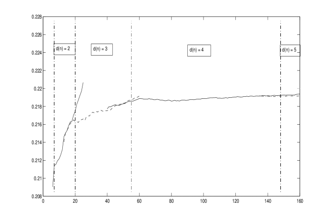
Figure 1: Optimal functional quantization of the Brownian motion. $\displaystyle n\mapsto\log n\,(e_{{}_{n}}(W,L^{2}_{{}_{T}}))^{2}$, $n\!\in\{6,\ldots,160\}$ for blocksizes $d_{n}\in\{2,3,4,5\}$. Vertical dashed lines: critical dimensions for $d^{\ast}_{n}$, $e^{2}\approx 7$, $e^{3}\approx 20$, $e^{4}\approx 55$, $e^{5}\approx 148$.

The main point is of course that the dimension $d^{\ast}_{n}$ is unknown. However (see Figure 1), one clearly verifies on small values of $n$ that in the case of the Brownian Motion, i.e $b=2$ the conjecture ($d^{\ast}_{n}\sim\log n$) is most likely true. Then for higher values of $n$ one relies on it to shift from one dimension to another following the rule $d^{\ast}_{n}=d$, $n\!\in\{e^{d},\ldots,e^{d+1}-1\}$.

3.2.1 A toolbox for quantization optimization: a short overview

Here is a short overview of stochastic optimization methods to compute optimal or at least locally optimal quantizers in finite dimension. For more details we refer to [16] and the references therein. Let $Z\stackrel{{\scriptstyle d}}{{=}}{\cal N}(0;I_{d})$ and denote by $D^{Z}_{n}(x)$ the distortion function, which is in fact the squared quantization error of a quantizer $x\!\in H^{n}=({R}^{d})^{n}$ in $n$-tuple notation, i.e.

$$D^{Z}_{n}:H^{n}\rightarrow{R},\quad x\mapsto{E}\min_{1\leq i\leq n}\lVert Z-x_{i}\rVert_{H}^{2}.$$

Competitive Learning Vector Quantization ($CLVQ$). This procedure is a recursive stochastic approximation gradient descent based on the integral representation of the gradient $\nabla D^{Z}_{n}(x),\,x\!\in H^{n}$ of the distortion as the expectation of a local gradient and a sequence of i.i.d. random variates, i.e.

$$\forall\,x\in H^{n},\quad\nabla D^{Z}_{n}(x)={E}(\nabla D^{Z}_{n}(x,Z))\;\text{ and }\;Z_{k}\;\;i.i.d.,\;Z_{1}\stackrel{{\scriptstyle d}}{{=}}{\cal N}(0,I_{d})$$

for $\nabla D^{Z}_{n}(x)=\left(2\int_{C_{i}(x)}(x_{i}-\xi)\mathbb{P}_{Z}(d\xi)\right)_{1\leq i\leq n}$ and $\nabla D^{Z}_{n}(x,Z)=\left(2(x_{i}-Z)1_{C_{i}(x)}(Z)\right)_{1\leq i\leq n}$ so that, starting from $x(0)\!\in({R}^{d})^{n}$, one sets

$$\forall\,k\geq 0,\quad x(k+1) = x(k)-\frac{c}{k+1}\nabla D^{Z}_{n}(x(k),Z_{k+1})$$

where $c\!\in(0,1]$ is a real constant to be tuned. As set, this looks quite formal but the operating $CLVQ$ procedure consists of two phases at each iteration:

$(i)$ Competitive Phase: Search of the nearest neighbor $x(k)_{i*(k+1)}$ of $Z_{k+1}$ among the components of $x(k)_{i}$, $i=1,\ldots,n$ (using a “winning convention” in case of conflict on the boundary of the Voronoi cells).

$(ii)$ Cooperative Phase: One moves the winning component toward $\zeta_{k+1}$ using a dilatation $i.e.$ $x(k+1)_{i^{*}(k+1)}={\rm Dilatation}_{\zeta_{k+1},1-\frac{c}{k+1}}(x(k)_{i^{*}(k+1)})$.

This procedure is useful for small or medium values of $n$. For an extensive study of this procedure, which turns out to be singular in the world of recursive stochastic approximation algorithms, we refer to [14]. For general background on stochastic approximation, we refer to [8, 1].

The randomized “Lloyd I procedure”. This is the randomization of the stationarity based fixed point procedure since any optimal quantizer satisfies the stationarity property:

$$\widehat{Z}^{x(k+1)}={E}(Z\,|\,\widehat{Z}^{x(k)}),\qquad x(0)\subset{R}^{d}.$$

At every iteration the conditional expectation ${E}(Z\,|\,\widehat{Z}^{x(k)})$ is computed using a Monte Carlo simulation. For more details about practical aspects of Lloyd I procedure we refer to [16]. In [13], an approach based on genetic evolutionary algorithms is developed.

For both procedures, one may substitute a sequence of quasi-random numbers to the usual pseudo-random sequence. This often speeds up the rate of convergence of the method, although this can only be proved (see [9]) for a very specific class of stochastic algorithm (to which $CLVQ$ does not belong).

The most important step to preserve the accuracy of the quantization as $n$ (and $d^{\ast}_{n}$) increase is to use the so-called splitting method which finds its origin in the proof of the existence of an optimal $n$-quantizer: once the optimization of a quantization grid of size $n$ is achieved, one specifies the starting grid for the size $n+1$ or more generally $n+\nu$, $\nu\geq 1$, by merging the optimized grid of size $n$ resulting from the former procedure with $\nu$ points sampled independently from the normal distribution with probability density proportional to $\varphi^{\frac{d}{d+2}}$ where $\varphi$ denotes the p.d.f. of ${\cal N}(0;I_{d})$. This rather unexpected choice is motivated by the fact that this distribution provides the lowest in average random quantization error (see [2]).

As a result, to be downloaded on the website [18] devoted to quantization:

www.quantize.maths-fi.com

$\circ$ Optimized stationary codebooks for $W$: in practice, the $n$-quantizers $\alpha:=\alpha^{d^{\ast}_{n}}$ of the distribution $\otimes_{k=1}^{d^{\ast}_{n}}{\cal N}(0,\lambda_{k})$, $n\!=\!1$ up to $10\,000$ ($d^{\ast}_{n}$ runs from $1$ up to $9$).

$\circ$ Companion parameters:

    – distribution of $\widehat{W}^{\gamma}$: ${P}(\widehat{W}^{\gamma}\!=x_{i})={P}(\widehat{Z}_{d^{\ast}_{n}}^{\alpha}\!=\alpha_{i})$.

    – The quadratic quantization error: $\|W-\widehat{W}^{\gamma^{n}}\|_{L^{2}_{T}}$.

3.3 Application to the Brownian motion on $L^{2}([0,T],dt)$

We present in this subsection numerical results for the above quantizer designs applied to the Brownian motion $W$ on the Hilbert space $\bigl{(}L^{2}([0,T],dt),\lVert\cdot\rVert_{L^{2}_{T}}\bigr{)}$.

Recall that the eigenvalues of $C_{W}$ read

$$\lambda_{j}=\left(\frac{T}{\pi(j-1/2)}\right)^{2},\quad j\geq 1$$

and the eigenvectors

$$u_{j}=\sqrt{\frac{2}{T}}\sin(t/\sqrt{\lambda_{j}}),\quad j\geq 1$$

which imply a regularity index of $b=2$ for the regularly varying function

$$\varphi(x):=\left(\frac{T}{\pi}\right)^{2}x^{-2}.$$

Let $\alpha$ be a quantizer for $\bigotimes_{j=1}^{\infty}\mathcal{N}(0,\lambda_{j})$, then for $S^{-1}$ from (3.1)

$$\gamma:=S^{-1}\alpha=\Bigl{\{}t\mapsto\sqrt{\frac{2}{T}}\sum_{j\geq 1}a_{j}\sin\bigl{(}\pi(j-1/2)t/T\bigr{)}:(a_{1},a_{2},\dots)\in\alpha\Bigr{\}}$$ (3.6)

provides a quantizer for $W$, which produces the same quantization error as $\alpha$ and is stationary iff $\alpha$ is. Furthermore we can restrict w.l.o.g. to the case $T=1$.

Concerning the numerical construction of a quantizer for the Brownian motion we need access to precomputed stationary quantizers of $\bigotimes_{j=k_{i}+1}^{k_{i+1}}\mathcal{N}(0,\lambda_{j})$ and $\bigotimes_{j=k_{i}+1}^{k_{i+1}}\mathcal{N}(0,1)$ for all possible combinations of the block allocation problem. As soon as these quantizers are computed, we can perform the Block Allocation of the quantizer Designs to produce optimal Quantizers for $\bigotimes_{j=1}^{\infty}\mathcal{N}(0,\lambda_{j})$.

For the quantizers of Design I we used the stochastic algorithm from section 3.2, whereas for Designs II - IV we could employ deterministic procedures for the integration on the Voronoi cells with max. block lengths $l=2$ respectively $l=3$, which provide a maximum level of stationarity, i.e. $\lVert\nabla D_{n}\rVert\leq 1e^{-8}$.

n	$d_{n}$	${E}\lVert W-\widehat{W}^{\gamma^{\ref{des:single}}}\rVert^{2}_{L^{2}_{T}}$
1	1	0.5000
5	1	0.1271
10	2	0.0921
50	3	0.0558
100	4	0.0475
500	6	0.0353
1000	6	0.0318
5000	8	0.0258
10000	9	0.0238

Table 1: Quantizer Design I

n	$n_{i}$	$l_{i}$	${E}\lVert W-\widehat{W}^{\gamma^{\ref{des:FourierQuant}}}\rVert^{2}_{L^{2}_{T}}$
1	1	1	0.5000
5	5	1	0.1271
10	10	1	0.0921
50	$25\times 2=50$	$2+1=3$	0.0580
100	$50\times 2=50$	$2+1=3$	0.0492
500	$100\times 2=500$	$2+1=3$	0.0372
1000	$111\times 3\times 3=999$	$2+1+2=5$	0.0339
5000	$166\times 10\times 3=4980$	$2+2+2=6$	0.0276
10000	$208\times 12\times 4=9984$	$2+2+2=6$	0.0255
100000	$277\times 20\times 6\times 3=99720$	$2+2+2+2=8$	0.0206

Table 2: Quantizer Design II, $l=2$

n	$n_{i}$	$l_{i}$	${E}\lVert W-\widehat{W}^{\gamma^{\ref{des:NormalQuant}}}\rVert^{2}_{L^{2}_{T}}$
1	1	1	0.5000
5	5	1	0.1271
10	$5\times 2$	$1+1=2$	0.0984
50	$10\times 5=50$	$1+2=3$	0.0616
100	$12\times 4\times 2=96$	$1+1+1=3$	0.0513
500	$16\times 5\times 3\times 2=480$	$1+1+1+1=4$	0.0387
1000	$20\times 25\times 2=1000$	$1+2+1=5$	0.0350
5000	$26\times 8\times 8\times 3=4992$	$1+1+2+2=6$	0.0285
10000	$25\times 36\times 11=9900$	$1+2+3=6$	0.0264
100000	$33\times 55\times 11\times 5=99825$	$1+2+2+3=8$	0.0211

Table 3: Quantizer Design III, $l=3$

n	$n_{i}$	$m$	${E}\lVert W-\widehat{W}^{\gamma^{\ref{des:scalarQuant}}}\rVert^{2}_{L^{2}_{T}}$
1	1	1	0.5000
5	5	1	0.1271
10	$5\times 2$	$2$	0.0984
50	$12\times 4=48$	$2$	0.0616
100	$12\times 4\times 2=96$	$3$	0.0513
500	$16\times 5\times 3\times 2=480$	$4$	0.0387
1000	$23\times 7\times 3\times 2=966$	$4$	0.0352
5000	$26\times 8\times 4\times 3\times 2=4992$	$5$	0.0286
10000	$26\times 8\times 4\times 3\times 2\times 2=9984$	$6$	0.0264
100000	$34\times 10\times 6\times 4\times 3\times 2\times 2=97920$	$7$	0.0213

Table 4: Quantizer Design IV

The asymptotical performance of the quantizer designs in view of Theorem 2, i.e.

$$n\mapsto\log n\ {E}\lVert W-\widehat{W}^{\gamma}\rVert^{2}_{L_{T}^{2}}.$$

is presented in Figure 2, where the quantization coefficient is evaluated for the Brownian Motion on $[0,1]$ with $\varphi(j)=\pi^{-2}j^{.2}$ as

$$\Bigl{(}\frac{b}{2}\Bigr{)}^{b-1}\frac{b}{b-1}\pi^{-2}=\frac{2}{\pi^{2}}\approx 0.20264237...\ .$$

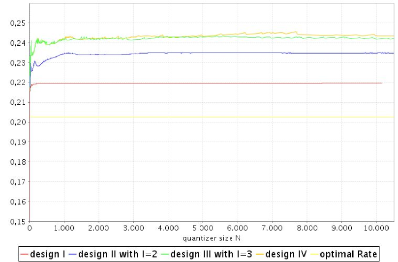
Figure 2: Asymptotics for $n\mapsto\log n\times{E}\lVert W-\widehat{W}^{\gamma}\rVert^{2}_{L^{2}}$ for the Designs I, II, III and IV.

As expected we have

$${E}\lVert W-\widehat{W}^{\gamma^{\ref{des:FourierQuant}}}\rVert^{2}_{L^{2}_{T}}\leq{E}\lVert W-\widehat{W}^{\gamma^{\ref{des:NormalQuant}}}\rVert^{2}_{L^{2}_{T}}\leq{E}\lVert W-\widehat{W}^{\gamma^{\ref{des:scalarQuant}}}\rVert^{2}_{L^{2}_{T}}$$

and by (3.5),

$$\log n\ {E}\lVert W-\widehat{W}^{\gamma^{\ref{des:scalarQuant}}}\rVert^{2}_{L^{2}_{T}}\stackrel{{\scriptstyle<}}{{\sim}}\frac{4C(1)+1}{2}\log n\ e_{n}(W)^{2}=5.9414\ldots\log n\ e_{n}(W)^{2}\sim 1.2040\ldots$$

assuming $C(1)=Q(1)$.

Although the Designs I, II and III are asymptotically equivalent, we can observe a great superiority of Designs I and II compared to Design III.

This is mainly caused by the better adaption to the rapidly decreasing sequence of the eigenvalues. To give an impression of this geometrical superior adaption, we illustrate the case $n=6$ in Figure 3.

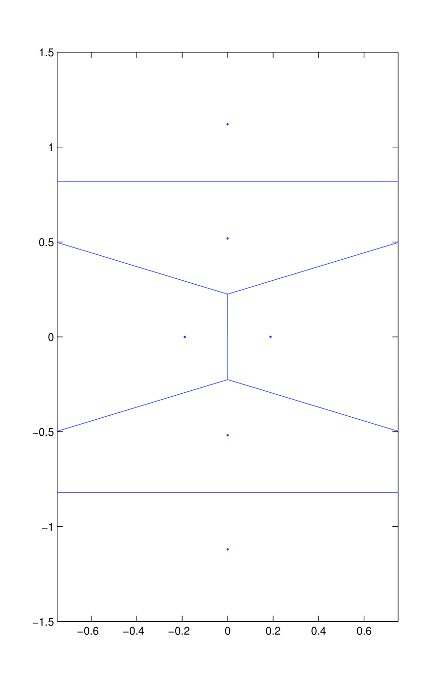
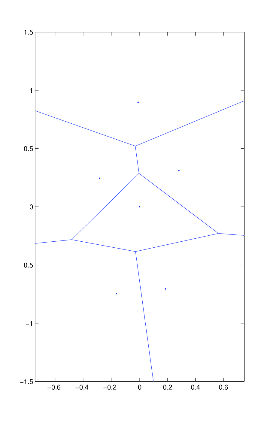
Figure 3: Quantizers of size $n=6$ for $\bigotimes_{j=1}^{\infty}\mathcal{N}(0,\lambda_{j})$ generated by Designs II, III and IV (from left to right) and projected on the eigenspace corresponding to $\lambda_{1}$ and $\lambda_{2}$

The quantizers for $\bigotimes_{j=1}^{\infty}\mathcal{N}(0,\lambda_{j})$ in the figure are projected onto the first two dimensions. Within that subspace, quantizer IV is a product quantizer of $\alpha^{1}\times\{0\}$, hence the rectangular shape of the Voronoi cells.

As quantizer III was formerly optimized for the symmetrically distribution $\mathcal{N}(0,I_{2})$, there are still to many points in the subspace generated by the eigenvector of $\lambda_{2}$, which cannot be accomplished by the weightening tensor product $\sqrt{\lambda^{(i)}}\otimes\alpha^{(i)}$.

Concerning quantizer II, we see the possibly best quantizer at level 6 for $\bigotimes_{j=1}^{\infty}\mathcal{N}(0,\lambda_{j})$, since the quantizer Design II produces the same quantizer for $N=6$ regardless of $l=2$ or $l=3$ and is therefore equivalent to Design I.

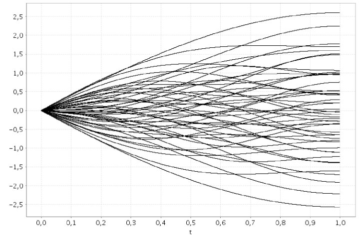
Figure 4: A stationary quantizer for $W$ on $L^{2}([0,1],dt)$ generated by Design I, size $n=50$ and $d^{\ast}_{n}=3$

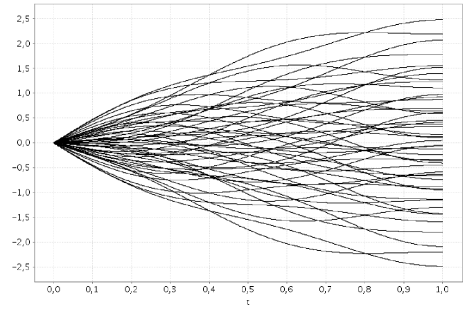
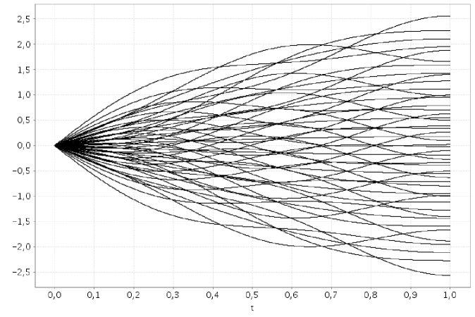
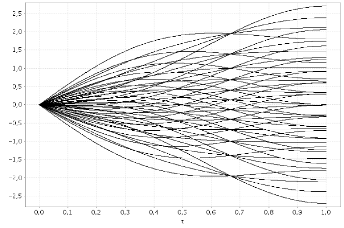
Figure 5: Stationary quantizers of size $n=50$ for $W$ on $L^{2}([0,1],dt)$ generated by Designs II - IV (from top to bottom). See also tables 2 - 4.

3.4 Application to Riemann-Liouville processes

We consider Riemann-Liouville processes in $H=L^{2}([0,T],dt)$. For $\rho\in(0,\infty)$, the Riemann-Liouville process $X^{\rho}=(X^{\rho}_{t})_{t\in[0,T]}$ on $[0,T]$ is defined by

$$X^{\rho}_{t}:=\int^{t}_{0}(t-s)^{\rho-\frac{1}{2}}dW_{s}$$ (3.7)

where $W$ is a standard Brownian motion.

Its covariance function is given by

$${E}\,X^{\rho}_{s}X^{\rho}_{t}=\int^{s\wedge t}_{0}(t-r)^{\rho-\frac{1}{2}}(s-r)^{\rho-\frac{1}{2}}dr.$$ (3.8)

Using $\rho\wedge\frac{1}{2}$-Hölder continuity of the application $t\mapsto X^{\rho}_{t}$ from [0,T] into $L^{2}({P})$ and the Kolmorogov criterion one checks that $X^{\rho}$ has a pathwise continuous modification so that we may assume without loss of generality that $X^{\rho}$ is pathwise continuous. In particular, $X^{\rho}$ can be seen as a centered Gaussian random vector with values in

$$H=L^{2}([0,T],dt).$$

The following high-resolution formula is a consequence of a theorem by Vu and Gorenflo [19] on singular values of Riemann-Liouville integral operators

$$R_{\beta}\,g(t)=\frac{1}{\Gamma(\beta)}\int^{t}_{0}(t-s)^{\beta-1}g(s)ds,\hskip 28.45274pt\beta\in(0,\infty).$$ (3.9)

For every $\rho\in(0,\infty)$,

$$e_{n}(X^{\rho})\sim T^{\rho+1/2}\pi^{-(\rho+\frac{1}{2})}(\rho+1/2)^{\rho}(\frac{2\rho+1}{2\rho})^{1/2}\Gamma(\rho+1/2)(\log n)^{-\rho}\;\mbox{ as }\;n\rightarrow\infty.$$ (3.10)

This can be seen as follows. For $\beta>1/2$, the Riemann-Liouville fractional integral operator $R_{\beta}$ is a bounded operator from $L^{2}([0,T],dt)$ into $L^{2}([0,T],dt)$. The covariance operator

$$C_{\rho}:L^{2}([0,T],dt)\rightarrow L^{2}([0,T],dt)$$

of $X^{\rho}$ is given by the Fredholm transformation

$$C_{\rho}g(t)=\int^{T}_{0}g(s){E}X^{\rho}_{s}X^{\rho}_{t}ds.$$

Using (3.8), one checks that $C_{\rho}$ admits a factorization

$$C_{\rho}=S_{\rho}S^{*}_{\rho},$$

where

$$S_{\rho}=\Gamma(\rho+1/2)R_{\rho+\frac{1}{2}}.$$

Consequently, it follows from Theorem 1 in [19] that the eigenvalues $\lambda_{1}\geq\lambda_{2}\geq\ldots>0$ of $C_{\rho}$ satisfy

$$\lambda_{j}\sim T^{2\rho+1}\Gamma(\rho+1/2)^{2}(\pi j)^{-(2\rho+1)}\;\mbox{ as }\;j\rightarrow\infty.$$ (3.11)

Now (3.10) follows from Theorem 1 (with $\varphi(x)=T^{2\rho+1}\Gamma(\rho+1/2)^{2}\pi^{-b}x^{-b}$ and $b=2\rho+1)$.

An immediate consequence for fractionally integrated Brownian motions on $[0,T]$ defined by

$$Y^{\beta}_{t}:=\frac{1}{\Gamma(\beta)}\int^{t}_{0}(t-s)^{\beta-1}W_{s}ds$$ (3.12)

for $\beta\in(0,\infty)$ is as follows.

For every $\beta\in(0,\infty),$

$$e_{n}(Y^{\beta})\sim T^{\beta+1}\pi^{-(\beta+1)}(\beta+1)^{\beta+\frac{1}{2}}(\frac{2\beta+2}{2\beta+1})^{1/2}(\log n)^{-(\beta+\frac{1}{2})}\;\mbox{ as }\;n\to\infty.$$

In fact, for $\rho>1/2$, the Ito formula yields

$$X^{\rho}_{t}=(\rho-\frac{1}{2})\int^{t}_{0}(t-s)^{\rho-\frac{3}{2}}W_{s}ds.$$

Consequently,

$$Y^{\beta}_{t}=\frac{1}{\beta\Gamma(\beta)}\beta\int^{t}_{0}(t-s)^{\beta+\frac{1}{2}-\frac{3}{2}}W_{s}ds=\frac{1}{\Gamma(1+\beta)}X_{t}^{\beta+\frac{1}{2}}.$$

The assertion follows.

One further consequence is a precise relationship between the quantization errors of Riemann-Liouville processes and fractional Brownian motions. The fractional Brownian motion with Hurst exponent $\rho\in(0,1]$ is a centered pathwise continuous Gaussian process $Z^{\rho}=(Z^{\rho}_{t})_{t\in[0,T]}$ having the covariance function

$${E}\,Z^{\rho}_{s}Z^{\rho}_{t}=\frac{1}{2}(s^{2\rho}+t^{2\rho}-\mid s-t\mid^{2\rho}).$$ (3.13)

For every $\rho\in(0,1)$,

$$e_{n}(X^{\rho})\sim\frac{\Gamma(\rho+1/2)}{(\Gamma(2\rho+1)\sin(\pi\rho))^{1/2}}e_{n}(Z^{\rho})\;\mbox{ as }\;n\rightarrow\infty.$$ (3.14)

In fact, by [11], we have

$$e_{n}(Z^{\rho})\sim T^{\rho+1/2}\pi^{-(\rho+\frac{1}{2})}(\rho+1/2)^{\rho}\left(\frac{2\rho+1}{2\rho}\right)^{1/2}(\Gamma(2\rho+1)\sin(\pi\rho))^{1/2}(\log n)^{-\rho},n\rightarrow\infty.$$

Combining this formula with (3.10) yields the assertion (3.14)

Observe that strong equivalence $e_{n}(X^{\rho})\sim e_{n}(Z^{\rho})$ as $n\rightarrow\infty$ is true for exactly two values of $\rho\in(0,1)$, namely for $\rho=1/2$ where even $e_{n}(X^{1/2})=e_{n}(Z^{1/2})=e_{n}(W)$ and, a bit mysterious, for $\rho=0.81557\ldots$

The basic example (among Riemann-Liouville processes) is $X^{1/2}=W$ and $H=L^{2}([0,T],dt)$, where

$$\lambda_{j}=T^{2}(\pi(j-1/2))^{-2},\;u_{j}(t)=\sqrt{\frac{2}{T}}\;\mbox{sin}\,\left(t/\sqrt{\lambda_{j}}\right),\;j\geq 1$$ (3.15)

(see Section 3.3).

Since for $\delta,\rho\in(0,\infty)$,

$$X^{\delta+\rho}=\frac{\Gamma(\delta+\rho+\frac{1}{2})}{\Gamma(\rho+\frac{1}{2})}R_{\delta}(X^{\rho}),$$

one gets expansions of $X^{\delta+\rho}$ from Karhunen-Loève expansions of $X^{\rho}$. In particular,

$$X^{\delta+\frac{1}{2}}=\Gamma(\delta+1)\sum\limits^{\infty}_{j=1}\sqrt{\lambda_{j}}\xi_{j}R_{\delta}(u_{j}).$$

However, the functions $R_{\delta}(u_{j}),j\geq 1$, are not orthogonal in $H$ so that the nonzero correlation between the components of $(\xi^{(j)}-\widehat{\xi^{(j)}})$ prevents the previous estimates for ${E}\|X-\widehat{X}^{n}\|^{2}$ given in Lemma 1 from working in this setting in the general case.

However, when $l=1$ (scalar product quantizers made up with blocks of fixed length $l=1$, see Design I), one checks that these estimates still stand as equalities since orthogonality can now be substituted by the independence of $\xi_{j}-\hat{\xi}_{j}$ and stationarity property (2.2) of the quantizations $\hat{\xi}_{j},j\geq 1$. It is often good enough for applications to use scalar product quantizers (see [10], [17]). If, for instance $\delta=1$, then

$$X:=X^{3/2}=\sum\limits^{\infty}_{j=1}\sqrt{\lambda_{j}}\xi_{j}R_{1}(u_{j}),$$

where

$$R_{1}(u_{j})(t)=\sqrt{\frac{2\lambda_{j}}{T}}(1-\cos(t/\sqrt{\lambda_{j}})).$$

Note that $\displaystyle\|R_{1}(u_{j})\|^{2}=T^{2}\mu_{j}(3-4(-1)^{j-1}\sqrt{\mu_{j}}),\;j\geq 1$, where $\lambda_{j}=T^{2}\mu_{j}$. Set

$$\hat{X}^{n}=\sum\limits^{m}_{j=1}\sqrt{\lambda_{j}}\hat{\xi}_{j}R_{1}(u_{j}).$$

The quantization $\widehat{X}^{n}$ is non Voronoi (it is related to the Voronoi tessellation of $W$) and satisfies

$${E}\|X-\widehat{X}^{n}\|^{2}=\sum^{m}_{j=1}T^{4}\mu^{2}_{j}(3-4(-1)^{j-1}\sqrt{\mu_{j}})e_{n_{j}}(N(0,1))^{2}+\sum_{j\geq m+1}T^{4}\mu^{2}_{j}(3-4(-1)^{j-1}\sqrt{\mu_{j}}).$$ (3.16)

It is possible to optimize the (scalar product) quantization error using this expression instead of (2.7). As concerns asymptotics, if the parameters are tuned following (2.8)-(2.10) with $l=1$ and $\lambda_{j}$ replaced by

$$\nu_{j}:=T^{4}\mu^{2}_{j}(3+4\sqrt{\mu_{j}})\sim 3\pi^{-4}j^{-4}\quad\mbox{ as }\quad n\to\infty,$$

and using (3.10) gives

$$({E}\,\|X-\hat{X}^{n}\|^{2})^{1/2}\stackrel{{\scriptstyle<}}{{\sim}}\left(\frac{3(12C(1)+1)}{4}\right)^{1/2}e_{n}(X)\;\mbox{ as }\;n\rightarrow\infty.$$ (3.17)

Numerical experiments seem to confirm that $C(1)=Q(1)$. Since $Q(1)=\pi\sqrt{3}/2$ (see [5], p. 124), the above upper bound is then

$$\left(\frac{3(6\pi\sqrt{3}+1)}{4}\right)^{1/2}=5.02357\ldots$$

References

- [1] A. Benveniste, P. Priouret, and M. Métivier. Adaptive algorithms and stochastic approximations. Springer-Verlag New York, Inc., 1990.
- [2] P. Cohort. Limit theorems for random normalized distortion. Ann. Appl. Probab., 14(1):118–143, 2004.
- [3] S. Dereich. High resolution coding of stochastic processes and small ball probabilities. PhD thesis, TU Berlin, 2003.
- [4] A. Gersho and R.M. Gray. Vector Quantization and Signal Compression. Kluwer, Boston, 1992.
- [5] S. Graf and H. Luschgy. Foundations of Quantization for Probability Distributions. Lecture Notes in Mathematics 1730. Springer, Berlin, 2000.
- [6] S. Graf and H. Luschgy. The point density measure in the quantization of self-similar probabilities. Math. Proc. Cambridge Phil. Soc., 138(3):513–531, 2005.
- [7] R.M. Gray and D.L. Neuhoff. Quantization. IEEE Trans. Inform., 44:2325–2383, 1998.
- [8] H. J. Kushner and G.G. Yin. Stochastic approximation algorithms and applications. Applications of Mathematics. 35. Berlin: Springer., 1997.
- [9] B. Lapeyre, G. Pagès, and K. Sab. Sequences with low discrepancy. generalization and application to robbins-monro algorithm. Statistics, 21(2):251–272, 1990.
- [10] H. Luschgy and G. Pagès. Functional quantization of stochastic processes. J. Funct. Anal., 196:486–531, 2002.
- [11] H. Luschgy and G. Pagès. Sharp asymptotics of the functional quantization problem for gaussian processes. Ann.Probab., 32:1574–1599, 2004.
- [12] H. Luschgy and G. Pagès. Sharp asymptotics of the kolmorogov entropy for gaussian measures. J. Funct. Anal., 212:89–120, 2004.
- [13] M. Mrad and S. Ben Hamida. Optimal quantization: Evolutionary algorithm vs stochastic gradient. In JCIS, 2006.
- [14] G. Pagès. A space vector quantization method for numerical integration. Journal of Applied and Computational Mathematics, 89:1–38, 1997.
- [15] G. Pagès, H. Pham, and J. Printems. Optimal quantization methods and applications to numerical methods and applications in finance. In S. Rachev, editor, Handbook of Computational and Numerical Methods in Finance, pages 253–298. Birkhäuser, 2004.
- [16] G. Pagès and J. Printems. Optimal quadratic quantization for numerics: the gaussian case. Monte Carlo Methods and Applications, 9(2):135–166, 2003.
- [17] G. Pagès and J. Printems. Functional quantization for numerics with an application to option pricing. Monte Carlo Methods and Applications, 11(4):407–446, 2005.
- [18] G. Pagès and J Printems. www.quantize.maths-fi.com. website devoted to quantization, 2005. maths-fi.com.
- [19] Vu Kim Tuan and R. Gorenflo. Asymptotics of singular values of volterra integral operators. Numer. Funct. Anal. and Optimiz., 17:453–461, 1996.