Phase coherence in an ensemble of uncoupled limit-cycle oscillators receiving common Poisson impulses

Abstract

An ensemble of uncoupled limit-cycle oscillators receiving common Poisson impulses shows a range of non-trivial behavior, from synchronization, desynchronization, to clustering. The group behavior that arises in the ensemble can be predicted from the phase response of a single oscillator to a given impulsive perturbation. We present a theory based on phase reduction of a jump stochastic process describing a Poisson-driven limit-cycle oscillator, and verify the results through numerical simulations and electric circuit experiments. We also give a geometrical interpretation of the synchronizing mechanism, a perturbative expansion to the stationary phase distribution, and the diffusion limit of our jump stochastic model.

I Introduction

The improvement in response reproducibility of a system receiving identical fluctuating drive has received much attention recently  Roy ; Mainen-Sejnowski ; Royama ; Binder-Powers ; Galan ; Toral ; Zhou-Kurths ; Pakdaman ; Teramae-Dan ; Goldobin-Pikovsky ; Nagai-Nakao ; Nakao-Arai ; Nakao-Arai-Kawamura ; Lin ; Pikovsky-R-K1 . With a constant input signal, many systems composed of identical elements in an ensemble show unreliable response due to noise after starting from similar initial conditions, while a fluctuating drive greatly improves response reproducibility. This general phenomenon is observed in various guises throughout nature. Uncoupled lasers driven by a common master laser with a fluctuating output produce highly correlated output intensities Roy . In the rat neocortical neuron Mainen-Sejnowski , action potential (spike) generation times over many trials coincide when a fluctuating current is delivered to the soma. Synchronized firings in vivo in the cat spinal motoneurons Binder-Powers , and in neurons of the olfactory bulbs in mice Galan have also been reported. Population density correlation among spatially separated species, known as the Moran effect Royama , is a general phenomenon seen in many different organisms in the troposphere. The phenomenon has also been found in chaotic oscillators Toral ; Zhou-Kurths , where synchronization of the generalized phase has been observed, and is known as noise-induced chaotic synchronization. Common forcing may also lead to a decrease in response reproducibility Pikovsky-R-K1 ; Goldobin-Pikovsky ; Nagai-Nakao ; Nakao-Arai ; Lin ; Tass ; Hudson .

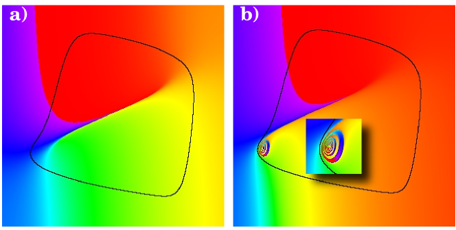
Figure 1: (Color online) Asymptotic phase for FHN oscillator with limit cycle in black. $I_{0}=0.8$ and $0.34$ in (a), (b), respectively. The center of the spiral in (b) occurs at the intersection of the nullclines, and is the remnant of a destabilized fixed point as the oscillator passes through a subcritical Hopf bifurcation where $I_{0}$ is the bifurcation parameter.

Let us first illustrate with examples the phase coherence phenomenon induced by fluctuating drive. Figures 1 and 11 show the orbit of unperturbed limit-cycle oscillators obtained numerically and experimentally, and Figs. 2 and 14 show the effect of common impulses on an ensemble of such oscillators. Though the oscillators do not interact with each other, they exhibit phase synchronization and desynchronization depending on the impulse intensity and oscillator characteristics. Knowledge of the response of the oscillator to an impulsive perturbation is sufficient to understand the observed coherence phenomena, as we will clarify in this paper.

Several previous studies have demonstrated this phenomenon for various driving signals and oscillators Teramae-Dan ; Goldobin-Pikovsky ; Nagai-Nakao ; Nakao-Arai ; Nakao-Arai-Kawamura ; Lin by using the phase reduction method for limit cycles Winfree ; Kuramoto . In particular, the case where the fluctuating signal is a sequence of random impulses has been investigated in Pikovsky, Rosenblum and Kurths (Pikovsky-R-K1 , Sec. 15 and references therein) and by ourselves Nakao-Arai . Using random phase maps, it is argued that synchronization always occurs for general limit cycles when sufficiently weak additive random impulses are given, and desynchronization can also occur when the impulse intensity is finite.

In this article, we generalize our previous argument through a refined formulation in terms of Poisson-driven Markov processes Snyder , also known as jump processes Hanson , which enables us to systematically perform phase reduction and linear stability analysis of our impulse-driven oscillators for general multiplicative coupling. The oscillator response to the impulses is expressed as a function called the phase response curve (PRC) Winfree ; Kuramoto , which is a very basic quantity of limit-cycle oscillators measured in every experiment, and the coherent behavior that arises from the common impulse can be deduced once the PRC is obtained. We present a criteria for predicting when each of the above coherence phenomenon can be expected from the application of common impulses, and test the predictions quantitatively using numerical simulation and an electric circuit experiment. We measure the PRC for a typical limit-cycle oscillator described by a set of ordinary differential equations, and for an electrical limit-cycle oscillator. We then compare the rate of synchronization or desynchronization as predicted by the Lyapunov exponent obtained from the PRC in both numerical simulation and experiment. We also give a simple geometrical explanation of the synchronization as a consequence of the stability of the limit cycle, a perturbative expansion to the phase distribution of a single oscillator, and a derivation of the diffusion limit of the jump process describing our impulse-driven limit-cycle oscillators in the Appendix.

II Theory

In this section, we present linear stability analysis of the impulse-driven oscillator through phase reduction of the jump stochastic differential equation describing the model. Similar analyses have been performed based on random phase map description for a simple sinusoidal phase map in Ref. Pikovsky-R-K1 , Sec. 15, and for more general phase maps derived from the phase reduction of limit cycles in Ref. Nakao-Arai , which gave formulas relating the Lyapunov exponent to the functional form of the phase maps and predicted synchronization and desynchronization of uncoupled oscillators driven by common random additive impulses. Our reformulation based on the stochastic jump process given in this section provides a simple and systematic treatment of the impulse-driven limit cycle oscillator for general multiplicative coupling, which quantitatively relates the Lyapunov exponents, the PRCs, and the phase-space structure (isochrons Winfree ) in a mathematically transparent way, starting from a general dynamical equation describing impulse-driven limit cycles. It also incorporates the effect of different stochastic interpretations for the random impulses. Using our new formulation, we derive the classical results in a more general way and argue the possibility of clustered states for multiplicative impulses.

II.1 Model

We consider an $N$-oscillator ensemble receiving a common sequence of random Poisson impulses. The equation for the $\alpha$-th oscillator is

$$\dot{\bm{X}}^{(\alpha)}(t)=\bm{F}(\bm{X}^{(\alpha)})+\sum_{n=1}^{N(t)}\bm{\sigma}(\bm{X}^{(\alpha)},\bm{c}_{n})h(t-t_{n}),$$ (1)

where $\alpha=1,\cdots,N$, $\bm{X}^{(\alpha)}(t)\in\bm{R}^{M}$ is the oscillator state at time $t$, $\bm{F}(\bm{X}^{(\alpha)}):\bm{R}^{M}\to\bm{R}^{M}$ the dynamics of a single oscillator, $N(t)$ the number of received impulses up to time $t$, ${t_{n}}$ the arrival time of the $n$-th impulse, $\bm{c}_{n}\in\bm{R}^{K}$ the intensity and direction, or mark Snyder ; Hanson , of the $n$-th impulse, $\bm{\sigma}(\bm{X}^{(\alpha)},\bm{c}):\bm{R}^{M}\times\bm{R}^{K}\to\bm{R}^{M}$ is the coupling function describing the effect of an impulse to $\bm{X}^{(\alpha)}(t)$, and $h(t-t_{n})$ is the unit impulse ($\int^{\infty}_{-\infty}h(t-t_{n})dt=1$) whose waveform is localized at the event time $t_{n}$. We denote the rate of the Poisson impulses as $\lambda$, namely, the mean interval between the impulses is $1/\lambda$.

In the absence of impulses, we assume that each oscillator obeys the same dynamics, with a single stable limit cycle solution $\bm{X}_{0}(t)$ of period $T$ in phase space. In the following, we omit the oscillator index $\alpha$ as the ensemble is composed of identical uncoupled elements, and our discussion involves only the linear stability of an individual oscillator.

II.2 Jump stochastic differential equation

We pose the problem as a Poisson-driven Markov process, or stochastic jump process. We regard the impulse as an event of zero-temporal width, so that the temporal correlation of the impulses vanishes. The resulting discontinuous oscillator dynamics can be described by a stochastic-integro differential equation, or jump stochastic differential equation (jump SDE), for a marked Poisson point process Snyder ; Hanson . Some properties of the jump SDE are given in Appendix A.

There are two ways we may interpret the impulse term in the original ordinary differential equation (1), which we call Ito and Stratonovich pictures for convenience. The Ito-picture assumes the impulsive term in the original Eq. (1) as being point-like impulses, which gives rise to discontinuous system dynamics with jumps. The Stratonovich-picture assumes the impulsive term in the original Eq. (1) as a limit of short but continuous waveforms of non-zero width, thus requiring that we find the limit of the system response as the impulses are shrunk to $0$ width.

Both pictures lead to the same jump SDE for the phase variable:

$$d\bm{X}(t)=\bm{F}(\bm{X})dt+\int_{\bm{c}}\bm{g}(\bm{X},\bm{c})M(dt,d\bm{c}),$$ (2)

which is always interpreted in the Ito sense. Here, $M(dt,d\bm{c})$ represents a Poisson random measure, which gives the number of incident points during $[t,t+dt]$ having the mark $[\bm{c},\bm{c}+d\bm{c}]$, whose expectation is

$$\langle M(dt,d\bm{c})\rangle=\lambda dtp(\bm{c})d\bm{c},$$ (3)

where $\lambda$ is the rate of the Poisson process and $p(\bm{c})$ is the probability density function (PDF) of the marks $\bm{c}$, and the integral is over the mark space (Ref. Snyder ; Hanson , Appendix A). The oscillator response $\bm{g}(\bm{X},\bm{c})$ to a given impulse with mark $\bm{c}$ is different between the two pictures when the effect of the impulse $\bm{\sigma}(\bm{X},\bm{c})$ is multiplicative. When the full oscillator dynamics is reduced to phase dynamics, the phase response is slightly altered, as we see later.

II.2.1 Ito picture

We interpret the common impulse $h(t-t_{n})$ in the original Eq. (1) to be zero-width from the outset. When an impulse $\bm{c}$ is received at time $t$, the state of the oscillator jumps discontinuously from $\bm{X}$ to $\bm{X}+\bm{\sigma}(\bm{X},\bm{c})$. This interpretation gives a jump SDE of the form

$$d\bm{X}(t)=\bm{F}(\bm{X})dt+\int_{\bm{c}}\bm{\sigma}(\bm{X},\bm{c})M(dt,d\bm{c}).$$ (4)

Thus, $\bm{g}(\bm{X},\bm{c})=\bm{\sigma}(\bm{X},\bm{c})$.

II.2.2 Stratonovich picture

We interpret the impulse $h(t-t_{n})$ in the original Eq. (1) as having a continuous waveform of finite width and then shrink the impulse width to 0. The resulting continuous process can be approximated by a discontinuous jump SDE with a jump amplitude as determined by the canonical form of the Wong-Zakai theorem for jump processes as shown by Marcus Wong-Zakai ; Marcus . Defining the differential operator

$$\hat{D}=\sum_{l=1}^{M}\sigma_{l}(\bm{X},\bm{c})\frac{\partial}{\partial X_{l}},$$ (5)

the jump SDE is given by

$$d\bm{X}(t)=\bm{F}(\bm{X})dt+\int_{\bm{c}}\left[e^{\hat{D}}\bm{X}-\bm{X}\right]M(dt,d\bm{c}).$$ (6)

Thus, $\bm{g}(\bm{X},\bm{c})=e^{\hat{D}}\bm{X}-\bm{X}$ in this case.

Note that for additive impulses, $\bm{\sigma}(\bm{X},\bm{c})\equiv\bm{\sigma}(\bm{c})$, Eq. (4) and Eq. (6) take the same form because $e^{\hat{D}}\bm{X}-\bm{X}=\bm{\sigma}(\bm{c})$. Therefore, the difference in stochastic interpretation is not important in this case. For the linear multiplicative case, $\sigma_{k}(\bm{X},\bm{c})=c_{k}X_{k}$. It is easy to check that $g_{k}(\bm{X},\bm{c})=(e^{c_{k}}-1)X_{k}$. This expression for the instantaneous jump magnitude approximates the effect of an impulsive perturbation due to a short but finite-width impulse whose intensity in each direction is $c_{k}$. For more general multiplicative coupling, explicit expressions for $\bm{g}(\bm{X},\bm{c})$ are difficult to obtain.

II.3 Phase reduction

To facilitate theoretical analysis, we apply phase reduction Winfree ; Kuramoto to Eq. (2), assuming that the average time-interval between jump events is long compared to the relaxation time of the perturbation to the limit cycle orbit. An unperturbed oscillator executes periodic motion along its limit cycle, so its state can be described by one phase variable $\phi(t)=\phi(\bm{X}_{0}(t))\in[0,1)$ which constantly increases with frequency $\omega=1/T$, instead of the original $M$ variables.

Because the limit cycle is assumed to be globally stable, the orbit of any initial point $P$ off of the limit cycle will asymptotically approach the limit cycle. Thus, we can extend the definition of the phase $\phi$ to the whole phase space except at phase singular sets by identifying the set of points that asymptotically converge to the same orbit on the limit cycle with the same phase, called the isochron Winfree ; Kuramoto . In practice, if the orbit approaches a point on the limit cycle with phase $\phi$ to within some arbitrarily small distance after time $\tau$, we define the asymptotic phase of the initial point $P$ to be $(\phi-\tau/T)\mbox{ mod }1$, where $T$ is the period of the oscillator.

Now we perform phase reduction, which is mathematically a change of variables describing the system from $\bm{X}$ to $\phi=\phi(\bm{X})$, and is also an approximation of the function of $\bm{X}$ by the corresponding function of $\bm{X}_{0}(\phi)$. In this transformation, every value of $\bm{X}$ in the neighborhood of the limit-cycle attractor maps to a value of $\phi$ except at phase singular sets. Using the stochastic chain rule for the jump process (Refs. Snyder ; Hanson , Appendix A), we obtain

$$d\phi(t)=\omega dt+\int_{\bm{c}}\left[\phi\left(\bm{X}+\bm{g}(\bm{X},\bm{c})\right)-\phi(\bm{X})\right]M(dt,d\bm{c}),$$ (7)

which is not yet a closed equation for $\phi$. The map $\bm{X}\to\bm{X}+\bm{g}(\bm{X},\bm{c})$ describes the effect of an impulse received when an oscillator is at $\bm{X}$. Since we assume that the average interval between impulses is longer than the relaxation time of the perturbation to the limit cycle, we can evaluate the function of $\bm{X}$ using values of $\bm{X}_{0}$ on the limit cycle, for which the mapping $\phi\to\bm{X}_{0}$ is well defined. Replacing the $\bm{X}$ with $\bm{X}_{0}(\phi)$, we obtain

$$d\phi(t) \cong \omega dt+\int_{\bm{c}}\left[\phi\left(\bm{X}_{0}(\phi)+\bm{g}(\bm{X}_{0}(\phi),\bm{c})\right)-\phi\right]M(dt,d\bm{c})$$ (8)

$$= \omega dt+\int_{\bm{c}}G(\phi,\bm{c})M(dt,d\bm{c}),$$ (10)

which is now a closed equation for $\phi$. Here we introduced a function

$$G(\phi,\bm{c})=\phi\left(\bm{X}_{0}(\phi)+\bm{g}(\bm{X}_{0}(\phi),\bm{c})\right)-\phi,$$ (11)

which is the phase response curve (PRC) representing the change in asymptotic phase relative to an unperturbed oscillator caused by an impulse with mark $\bm{c}$ received at phase $\phi$. Since we consider a continuous dynamical system, $G(\phi,\bm{c})$ is continuous and periodic in $\phi$. If the jump amplitude $\bm{g}(\bm{X}_{0}(\phi),\bm{c})$ is small, $G(\phi,\bm{c})$ can be approximated as

$$G(\phi,\bm{c})\cong\bm{Z}(\phi)\cdot\bm{g}(\bm{X}_{0}(\phi),\bm{c}),$$ (12)

where

$$\bm{Z}(\phi)=\mbox{grad}_{\bm{X}}\phi({\bm{X}})|_{\bm{X}=\bm{X}_{0}(\phi)}$$ (13)

is the well-known phase sensitivity function that represents linear sensitivity of the phase to infinitesimal perturbations Winfree ; Kuramoto . In general, this linear relationship holds only for very weak impulses (see e.g. Nakao-Arai ). The PRC easily becomes a largely fluctuating function, which can even become jagged, e.g. near the bifurcation point.

Note that for our phase-reduction analysis of Poisson-driven limit cycles, the impulse intensity $\bm{c}$ need not be infinitesimally weak provided that the inter impulse intervals are sufficiently long, in contrast to the conventional phase-reduction analysis of limit cycles driven by continuous signals Teramae-Dan ; Goldobin-Pikovsky ; Nakao-Arai-Kawamura . It holds for largely fluctuating PRCs as well. By virtue of this fact, we can analyze desynchronization effect of random signals within the framework of a one-dimensional phase model, in contrast to Ref. Goldobin-Pikovsky , as we discuss below.

II.4 Linear stability of the synchronized state

Whether synchronization occurs among the oscillators depends on the stability of the synchronized state. To investigate the linear stability of the synchronized state with the application of common impulses, we focus on the time evolution of a small phase difference $\psi=\tilde{\phi}-\phi$ between phase $\phi$ and $\tilde{\phi}$ of two nearby orbits. From Eq. (8), the linearized evolution equation for $\psi$ is given by

$$d\psi(t)=\int_{\bm{c}}\psi\frac{\partial}{\partial\phi}G(\phi,\bm{c})M(dt,d\bm{c}).$$ (14)

Now we change variables to the logarithm of the absolute value of the phase difference, $y=\mbox{log}|\psi|$. Using the stochastic chain rule for the jump process, we obtain

$$dy(t) = \int_{\bm{c}}\left[\mbox{log}|\psi+\psi G^{\prime}(\phi,\bm{c})|-\mbox{log}|\psi|\right]M(dt,d\bm{c})$$ (15)

$$= \int_{\bm{c}}\mbox{log}|1+G^{\prime}(\phi,\bm{c})|M(dt,d\bm{c}),$$ (17)

where the prime(^′) denotes partial derivative by $\phi$. The average growth rate of the small phase difference is characterized by the Lyapunov exponent $\Lambda$. In this case, it is defined as

$$\Lambda = \lim_{T\to\infty}\frac{1}{T}\log\left|\frac{\psi(T)}{\psi(0)}\right|=\lim_{T\to\infty}\frac{y(T)-y(0)}{T}=\lim_{T\to\infty}\frac{1}{T}\int_{0}^{T}dy(t).$$ (18)

When $\Lambda$ is negative, the initial phase difference decays exponentially, so that the synchronized state is linearly stable. As usual, we postulate that the growing and shrinking of the phase difference is ergodic, namely, the long-time average slope of $y(t)$ coincides with the ensemble average of its local slope,

$$\lim_{T\to\infty}\frac{1}{T}\int_{0}^{T}dy(t)=\frac{\langle dy(t)\rangle}{dt},$$ (19)

where $\langle\cdots\rangle$ denotes ensemble average over the marked Poisson process. Note that an individual increment $dy(t)$ may exhibit discontinuous jumps of $O(1)$, but the ensemble average $\langle dy(t)\rangle$ is always of $O(dt)$. The expectation of the right-hand-side is calculated by replacing the dynamics of $\phi$ with the single-oscillator stationary PDF $p(\phi)$ of $\phi$, as

$$\langle dy(t)\rangle = \left\langle\int_{\bm{c}}\log\left|1+G^{\prime}(\phi(t),\bm{c})\right|M(dt,d\bm{c})\right\rangle$$ (20)

$$= \int d\phi p(\phi)\int_{\bm{c}}\log\left|1+G^{\prime}(\phi,\bm{c})\right|\langle M(dt,d\bm{c})\rangle$$ (22)

$$= \lambda dt\int_{0}^{1}d\phi p(\phi)\int_{\bm{c}}d\bm{c}p(\bm{c})\log\left|1+G^{\prime}(\phi,\bm{c})\right|,\;\;\;\;\;\;\;\;$$ (24)

where in the second line, the ensemble average is separated into a conditional expectation with fixed $\phi$ and average over $p(\phi)$ because the integration variable and stochastic driving term are statistically independent. Thus, the Lyapunov exponent $\Lambda$ is obtained as

$$\Lambda = \lambda\int_{0}^{1}d\phi p(\phi)\int_{\bm{c}}d\bm{c}p(\bm{c})\log\left|1+G^{\prime}(\phi,\bm{c})\right|,$$ (25)

which generalizes the result obtained by random phase maps in Refs. Pikovsky-R-K1 and  Nakao-Arai for general multiplicative coupling. The sign of the Lyapunov exponent depends on the shape of the PRC, $G(\phi,\bm{c})$. When $G^{\prime}(\phi,\bm{c})<-2$ or $G^{\prime}(\phi,\bm{c})>0$, the integrand, which gives the instantaneous growth rate of $\psi(t)$ at $\phi$, is positive. Such regions tend to expand the phase difference between two orbits. When $-2<G^{\prime}(\phi,\bm{c})<0$, the integrand is negative, and the phase difference between two orbits tends to shrink. Linear stability of the synchronized state is determined by the overall balance between these two effects.

For weak impulses, we can further simplify Eq. (25) by assuming that, on average, an oscillator is equally distributed on the limit-cycle, so $p(\phi)=1$. This is a reasonable assumption in most cases where the effect of impulses are small Nakao-Arai , as we discuss later in Appendix B. Under this approximation, the Lyapunov exponent $\Lambda$ can be simplified as

$$\Lambda=\lambda\int_{0}^{1}d\phi\int_{\bm{c}}d\bm{c}p(\bm{c})\mbox{log}|1+G^{\prime}(\phi,\bm{c})|.$$ (26)

Now, if the impulses are weak and the variation of the PRC $G(\phi,\bm{c})$ is sufficiently small in such a way that $-1<G^{\prime}(\phi,\bm{c})$ is always satisfied for all $\phi$ and $\bm{c}$, i.e. when $\phi+G(\phi,\bm{c})$ is a monotonically increasing function, $\Lambda$ can be bounded from above as Nagai-Nakao ; Nakao-Arai

$$\Lambda \leq \lambda\int_{0}^{1}d\phi\int_{\bm{c}}d\bm{c}G^{\prime}(\phi,\bm{c})p(\bm{c})=\lambda\int_{\bm{c}}p(\bm{c})d\bm{c}\left[G(\phi,\bm{c})\right]_{\phi=0}^{\phi=1}=0,$$ (27)

where we utilized the periodicity of $G(\phi,\bm{c})$ in $\phi$ and the inequality $\log(1+x)\leq x$. Thus, for weak impulses, small perturbations are always statistically stabilized when averaged over the limit cycle, so that common impulses shrink the phase difference, irrespective of the details of the oscillator. A geometrical interpretation of this stabilization mechanism is given in Appendix C.

By a Taylor expansion of Eq. (26), the Lyapunov exponent can be approximated for weak impulse as

$$\Lambda\cong\lambda\int_{0}^{1}d\phi\int_{\bm{c}}d\bm{c}p(\bm{c})\left[G^{\prime}(\phi,\bm{c})-\frac{G^{\prime}(\phi,\bm{c})^{2}}{2}\right]=-\frac{\lambda}{2}\int_{0}^{1}d\phi\int_{\bm{c}}d\bm{c}p(\bm{c})G^{\prime}(\phi,\bm{c})^{2}\leq 0,$$ (28)

where the first term drops out due to the periodicity of $G(\phi,\bm{c})$. At the lowest order approximation, $G(\phi,\bm{c})\simeq{\bm{Z}}(\phi)\cdot\bm{g}(\phi,\bm{c})\simeq\sum_{k=1}^{M}Z_{k}(\phi)\sigma_{k}(\phi,\bm{c})$, the approximate Lyapunov exponent $\Lambda$ is obtained as

$$\Lambda = -\frac{\lambda}{2}\sum_{k=1}^{M}\sum_{l=1}^{M}\int_{0}^{1}d\phi[Z_{k}^{\prime}(\phi)Z_{l}^{\prime}(\phi)\langle\sigma_{k}\sigma_{l}\rangle_{\bm{c}}(\phi)$$ (31)

$$+2Z_{k}^{\prime}(\phi)Z_{l}(\phi)\langle\sigma_{k}\sigma_{l}^{\prime}\rangle_{\bm{c}}(\phi)+Z_{k}(\phi)Z_{l}(\phi)\langle\sigma_{k}^{\prime}\sigma_{l}^{\prime}\rangle_{\bm{c}}(\phi)]$$

for both Ito and Stratonovich pictures of Eq. (1), where we introduced correlation functions $\langle\sigma_{k}\sigma_{l}\rangle_{\bm{c}}(\phi)=\int_{\bm{c}}d\bm{c}p(\bm{c})\sigma_{k}(\phi,\bm{c})\sigma_{l}(\phi,\bm{c})$, etc. As we derive in Appendix D, we obtain the same Lyapunov exponent in the diffusion limit of the jump process.

II.5 Clustered states

If the PRC possesses a symmetry

$$G(\phi,\bm{c})=G(\phi+\frac{1}{m},\bm{c})$$ (32)

where $m\in\bm{N}$ and $1/m<1$ (i.e. $m=2,3,4,\cdots$), the stability of the synchronized state (zero phase difference) also implies the existence of stable states separated in phase by $1/m$. Defining $\psi$ as a small deviation from such a state, we set

$$\psi=\phi^{\prime}-\phi-\frac{1}{m}.$$ (33)

The linear stability analysis of a state separated in phase by $1/m$ yields the same Eq. (14) when utilizing PRC symmetry, so that the resulting Lyapunov exponent $\Lambda$, Eq. (26), also takes the same value as that of the synchronized state.

If $\Lambda$ is negative, the phase difference between two orbits can stably take $m$ different values. When many identical oscillators are driven by common impulses and also by small independent disturbances in such a situation, the oscillators will eventually split into $m$ clusters. Any two oscillators inside the same group are synchronized, and those belonging to different clusters will take one of $m-1$ phase differences, $n/m$ where $n=1,\cdots,m-1$. We call this an $m$-cluster state. As we demonstrate later, symmetry in the original limit cycle results in symmetry of the corresponding PRC, leading to cluster states.

III Numerical simulation

In this section, we demonstrate synchronization, desynchronization, and clustering induced by common impulses by numerical simulations, and test our theoretical predictions quantitatively, using the FitzHugh-Nagumo (FHN) neural oscillator as an example. The effect of common random signals for uncoupled FHN oscillators have been discussed for Gaussian signals in Ref. Goldobin-Pikovsky and for a random telegraphic signal in Ref. Nagai-Nakao . However, quantitative comparison of the Lyapunov exponent predicted from the PRC with that directly measured from numerical simulations have not been fully done, especially in the desynchronization regime. In this section, we measure the PRC and the separation rate of nearby trajectories directly by numerical simulations, and quantitatively confirm the theoretical prediction based on the one-dimensional phase model. Results for the Stuart-Landau oscillator, which is qualitatively different from the FHN oscillator, is also given in Appendix E for comparison.

III.1 Model

For the simulation, we employ the FitzHugh-Nagumo (FHN) neural oscillator Koch as an example, described by the following set of equations:

$$\dot{u}(t) = \varepsilon(v+a-bu),$$ (34)

$$\dot{v}(t) = v-\frac{v^{3}}{3}-u+I_{0}+\sigma(v,c)\sum_{n=1}^{N(t)}h(t-t_{n})+\sqrt{D}\xi(t).\;\;\;\;\;\;\;\;\;$$ (35)

Here, parameters $\varepsilon,a,b$ are fixed at $\varepsilon=0.08$, $a=0.7$, $b=0.8$, and we use the parameter $I_{0}$ to control the oscillator characteristics. The last two terms of the equation for $v$ describe impulses and noises. The $h(t)$ is a common impulse with unit intensity, generated by a Poisson point process of constant-rate $\lambda$. The function $\sigma(v,c)$ describes $v$-dependent effect of the impulse to the oscillator (for simplicity, we do not consider the case where $c$ takes multiple values in the following). The $\xi(t)$ is a Gaussian white noise with intensity $D$ describing independent disturbances to the oscillators.

When both external disturbances are zero, a limit cycle exists for $I_{0}\in[0.331,1.419]$, which is created by a subcritical Hopf bifurcation at either limits of $I_{0}$. Figure 1 displays portraits of asymptotic phase for two values of $I_{0}$ in the absence of impulses and noises. At $I_{0}=0.8$, the period of the limit cycle is $T\approx 36.52$, and the oscillator has a smooth phase portrait as shown in Fig. 1(a). Near the bifurcation point, $I_{0}=0.34$, the period of the limit cycle is $T\approx 46.79$. The remnants of the destabilized fixed point exist at this parameter, as seen in Fig. 1(b). We define the origin of phase $\phi$ as the point where the variable $v$ passes through the $v=0.9$ line from below, where the FHN oscillator appears to emit a neuronal action potential.

III.2 Phase response curves

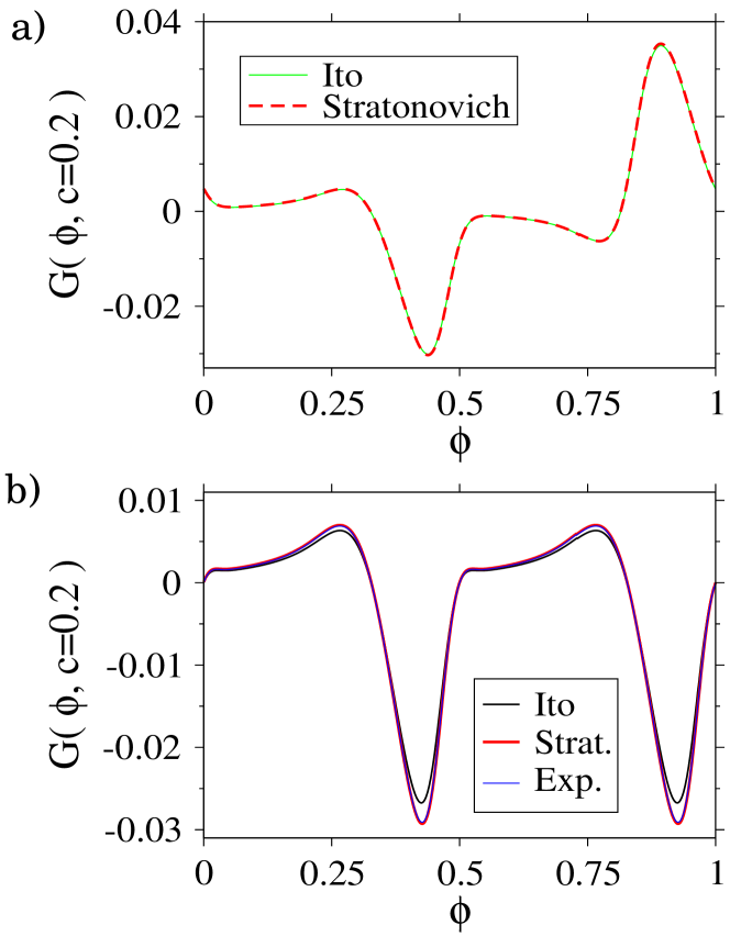
Figure 3: (Color online) Comparison of Ito vs. Stratonovich interpretations of Eq. (1) on the PRC $G(\phi,c)$ of FHN for an impulse whose jump size is $c=0.2$. (a) Additive impulse ($\sigma(v,c)=c$) and (b) Linear multiplicative impulse ($\sigma(v,c)=cv$). The curve “Ito” is calculated by affecting a discontinuous jump, i.e. impulse duration is $0$. The curve “Stratonovich” and “Strat.” is calculated by continuously changing $v$ using a narrow rectangular waveform of temporal width $0.0002$. The curve ”Exp.” is calculated using the Wang-Zakai-Marcus approximation for the continuous narrow impulse, namely, discontinuously changing the orbit by an amount $g(v,c)=(e^{c}-1)v$.

In simulation, we may use two algorithms corresponding to Ito and Stratonovich pictures of Eq. (1). If we treat the impulses as point events, allowing discontinuous jumps of the orbit of the oscillator, the results correspond to the Ito picture, Eq. (4). If we directly integrate short but non-zero-width continuous impulses, the results correspond to the Stratonovich picture, Eq. (6). When the effect of impulses are multiplicative, the PRC is different between the two interpretations. Figure 3 displays the PRCs obtained using Ito and Stratonovich pictures for additive impulses ($\sigma(v,c)=c$) and for linear multiplicative impulses ($\sigma(v,c)=cv$). For additive impulses, both algorithms give the same PRCs. In contrast, for multiplicative impulses, it is seen that a difference in the pictures has a small but visible effect on the PRC. Of course, the PRC obtained using Wong-Zakai-Marcus approximation coincides with that obtained in the Stratonovich picture. All the following simulations are done using the Stratonovich picture of the original Eq. (1), namely Eq. (6), using the Wong-Zakai-Marcus approximation of a continuous physical jump.

At $I_{0}=0.8$, the PRC for additive impulses is a smooth periodic function as shown in Fig. 4(a) for all values of the impulse intensity $c$, corresponding to the smooth phase portrait as shown in Fig. 1(a). In contrast, at $I_{0}=0.34$, the PRC can become jagged as shown in Fig. 4(b) for the impulse intensity $c$ in a certain range. This reflects the existence of the unstable focus, which looks like a spiral in Fig. 1(b). If the impulse intensity is in such a range that the orbit on the limit cycle is kicked into this region, an initial phase difference can grow quickly because the asymptotic phase in that region varies so rapidly.

III.3 Synchronization, desynchronization, and clustering

Raster plots of $N=20$ uncoupled FHN oscillators, Fig. 2, which indicate times that an oscillator passed through $\phi=0$, offer a qualitative picture of the phenomenon. Whether the impulse is introduced additively or multiplicatively, we find system and impulse parameters where phase synchronization occurs and where it does not. FHN oscillator has a large parameter range in $I_{0}$ and $c$ where common impulses cause the oscillators to synchronize, as shown in Fig. 2(a). However, near the bifurcation, common impulses sometimes accelerate the desynchronization of the oscillators, as shown in Fig. 2(b). These distinct behavior can be understood by examining the PRC of the FHN oscillator at each parameter value.

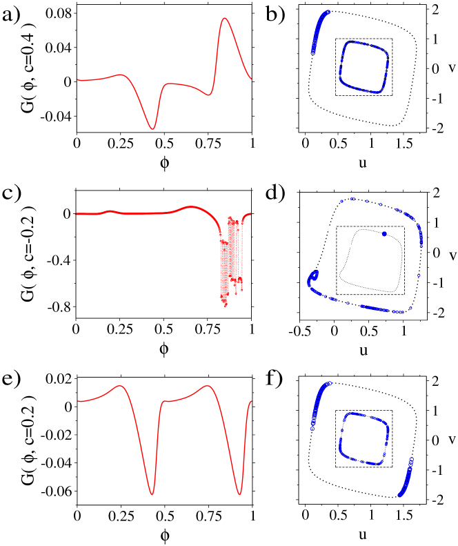
Figure 5: (Color online) Various PRCs and coherent states of FHN oscillators. (a), (c), (e) show PRCs $G(\phi,c)$, and (b), (d), (f) show corresponding phase-space diagrams of 200 oscillators a sufficient time after the initial condition shown in the insets. Poisson rate is $\lambda=1/4T$ for (a), (b), and (f), and independent noise is $D=5\times 10^{-6}$ for (b) and (f), and $D=9\times 10^{-9}$ for (d). The control parameter is $I_{0}=0.875$ for (a), (b), (e), (f), and $I_{0}=0.34$ for (c) and (d). For weak additive impulse, the PRC $G(\phi,c)$ is a periodic function, (a), and the 1-cluster (synchronized) state, (b), appears. At $I_{0}=0.34$, the PRC $G(\phi,c)$ becomes jagged when the additive impulse intensity is in a certain range as shown in (c), which often leads to common-impulse induced desynchronization, (d). For multiplicative impulse at $I_{0}=0.875$, a doubly periodic PRC $G(\phi,c)$, (e), leads to the 2-cluster state, (f).

Figure 5 summarizes the relation between the shapes of the PRC and the dynamics of the oscillator ensemble in the phase space. For a smooth PRC with relatively small amplitudes obtained at $I_{0}=0.8$ for additive impulse ($\sigma(v,c)=c$) as shown in Fig. 5(a), the oscillators groups together on the limit cycle, namely, synchronize with each other, by the application of common impulses, Fig. 5(b). For jagged PRC with strong amplitude fluctuations obtained by applying additive impulses near the bifurcation point $I_{0}=0.34$ as shown in Fig. 5(c), the oscillators undergo desynchronization by the application of common impulses and scatter along the limit cycle, as shown in Fig. 5(d). At the midway point between the subcritical bifurcation near $I_{0}=0.875$, the limit cycle becomes symmetric about $v=0$. If the impulse is applied in a linear multiplicative way ($\sigma(v,c)=cv$) in this $I_{0}$ region, the PRC becomes doubly periodic, as shown in Fig. 5(e), so that $2$-cluster state appears as shown in Fig. 5(f). Even when the parameters of the oscillators are slightly inhomogeneous, these dynamical behavior remain qualitatively unchanged .

In the present case for FHN oscillators, synchronization gradually occurs whereas desynchronization occurs suddenly due to the narrow jagged part of the PRC, typically obtained near the bifurcation point of the dynamics. However, we emphasize that desynchronization is not limited to such pathological situations. The PRC need not be rapidly fluctuating as long as intervals where the sufficiently steep slopes outweigh shallower slopes in Eq. (26). As we see in the next section, our electrical oscillator is of this type, where desynchronization occurs even though the oscillator is far from a bifurcation and the PRC is smoothly. As an example of this from a well-known system, we include results from the Stuart-Landau oscillator in Appendix E.

In Ref. Goldobin-Pikovsky , the mechanism for desynchronization is analyzed for FHN oscillators near the bifurcation point driven by finite strength white Gaussian forcing utilizing a two-variable phase-amplitude model to take into account the non-trivial transverse deviation from the limit cycle. In contrast, for our Poisson forcing case (and also for our previous case with random telegraphic forcing Nagai-Nakao ), we can eliminate the relaxation dynamics of the amplitude and isolate the effects of the phase perturbation, because the time-scale of oscillator relaxation back to the limit-cycle is assumed to be much shorter than the average impulse interval. We can thus stay within the framework of a single-variable phase model to describe both the synchronization and desynchronization, which elucidates the relation between the phase space structure (isochrons) and the desynchronization mechanism.

This desynchronization mechanism is qualitatively similar to the mechanism of the singular behavior in circadian clocks proposed by Winfree Winfree2 , who argued that the attenuation of the circadian rhythm by an external stimulus is due to the desynchronization of multiple independent circadian oscillators being kicked into the unstable focus of the limit cycle. In Ref. Tass , application of such a desynchronization mechanism to neural populations are discussed. Based on the same idea, the sudden desynchronization seen in coupled chemical oscillators when a common perturbation is administered at the correct timing is also reported Hudson . Recently, Ukai et al. Kobayashi performed a very clear experiment of this phenomenon using genetically engineered photosensitive cells exhibiting circadian oscillations.

III.4 Lyapunov exponents

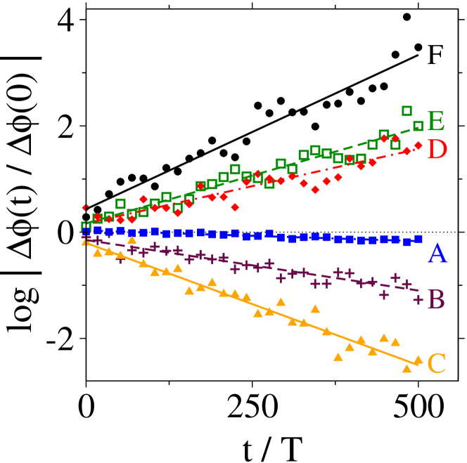
Figure 6: (Color online) Pairwise growth times of perturbations to FHN at $I_{0}=0.34$ for several values of the impulse intensity (A: $c=0.03$, B: $c=-0.6$, C: $c=0.4$, D: $c=0.2$, E: $c=-0.35$, and F: $c=-0.2$). Data was taken for 100-200 trials, each with an ensemble of 20 oscillators, and with Poisson impulse rate $\lambda=1/4T$. Slope of linear least-square fit gives the Lyapunov exponent.

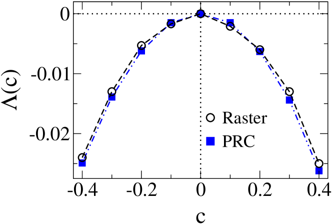
Figure 7: (Color online) Comparison of the Lyapunov exponents $\Lambda$ between the direct measurement from the raster plot and the theoretical prediction from the PRC for FHN with parameter $I_{0}=0.8$ driven by additive impulses of intensity $c$, and Poisson impulse rate $\lambda=1/4T$.

To quantitatively test our theory, we measured the Lyapunov exponent $\Lambda$ in two ways, from numerically obtained PRC $G(\phi,c)$ using Eq. (26) and by observing the growth rate of the phase difference of two oscillators with period $T$ using raster data, Fig. 2, for the case of common additive impulses. When the time difference $\Delta t$ between the respective $\phi=0$ events of two oscillators is below a threshold value ($\Delta t<0.02T$), we converted the time difference into $\Delta\phi(0)=\Delta t/T$, and followed the evolution by measuring subsequent $\Delta\phi(t)$. This was done for many oscillator pairs, and for a given $t$, we calculated the average of $\mbox{log}\left|\Delta\phi(t)/\Delta\phi(0)\right|$, as shown in Fig. 6 for $I_{0}=0.34$. The slope of this line gives $\Lambda$. Figures 7 and 8 show that Lyapunov exponents measured from the simulation data show good agreement with those measured from PRCs as shown in Figs. 4(a) and (b), respectively.

III.5 On-off intermittency and switching

While the instantaneous growth rate of the difference between two orbits, $\log|1+G^{\prime}(\phi,\bm{c})|$, may be a smoothly varying function with respect to phase $\phi$, since the common impulses are received at random phases, the separation between two oscillators can be considered a random multiplicative process driven by the fluctuations in the growth rate around the average Lyapunov exponent $\Lambda$. In the absence of any disturbances, complete synchronization results if the average effect of a common impulse causes small phase perturbations to shrink as indicated by the average Lyapunov exponent over the limit cycle, Eq. (26). However, if small disturbances exist in the system, fluctuations in the instantaneous growth rate can occasionally amplify a small deviation in the system, causing intermittent transient desynchronization.

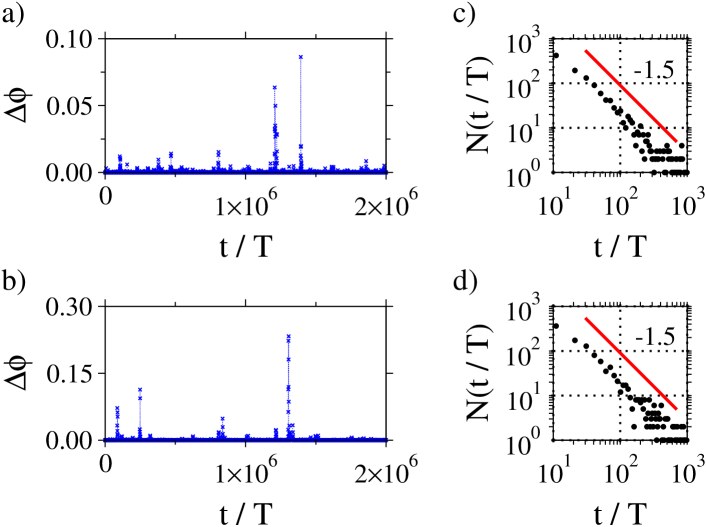
Figure 9: (Color online) On-off intermittency exhibited by 2 oscillators in synchronized ($I_{0}=0.8$, additive impulses with $c=0.1$), and clustered ($I_{0}=0.875$, linear multiplicative impulses with $c=0.1$) states. Independent noise with $D=9\times 10^{-9}$, and impulses with $\lambda=1/4T$ were used. Phase difference $\Delta\phi$ between the oscillators from stable configuration is small (laminar region) much of the time, but large occasional bursts occur. (a) long-time evolution of $\Delta\phi(t)$, which shows excursions away from the synchronized state. (b) distribution of laminar duration corresponding to (a) (arbitrary normalization). (c) long-time evolution of $\Delta\phi(t)$ from the $1/2$-out-of-phase clustered state, and (d) distribution of laminar duration corresponding to (c) (arbitrary normalization). Oscillators are considered to be in the laminar state when $\Delta\phi<0.0013$ away from synchronized or clustered states. Laminar distributions exhibit power laws with exponent $-1.5$. At this weak independent noise intensity, the phase difference between the oscillators takes only either $0$ or $1/2$ depending on the initial condition, and switching between the clustered state occurs is a very rare event.

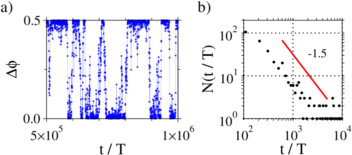
Figure 10: (Color online) Transition between clustered states for 2 oscillators. $\Delta\phi$ is the phase difference between the two oscillators. Poisson impulses with rate $\lambda=1/4T$ and $c=0.1$ was used. A larger independent noise with $D=3\times 10^{-4}$ is added in order to facilitate the transitions between single and 2-cluster states.

Figures 9 (a), (c) show an example of the large excursions away from the synchronized and clustered state respectively, while Fig. 9(b), (d) show the power-law PDF of laminar duration with the well-known exponent, $-1.5$ Fujisaka-Yamada ; Heagy ; Venkaratamani ; Pikovsky-R-K1 . When the system exhibits clustering, the same mechanism leads to switching for sufficiently strong independent noises, with a power-law PDF of the life-times of the states as shown in Fig. 10.

This fluctuation is known as modulational or on-off intermittency, which was first discovered in a pioneering work by Fujisaka and Yamada Fujisaka-Yamada on a system of coupled chaotic oscillators, and later clarified to be an ubiquitous feature of many nonlinear dynamical systems with a symmetry. The intermittency typically arises in synchronization problems of dynamical elements, where a dynamical variable acts as a time-dependent fluctuating driving parameter for a second variable Heagy ; Venkaratamani ; Pikovsky-R-K1 , for example in the synchronization of chaotic lasers Sauer-Kaiser , in spin-wave instabilities Roedelsperger , and in nematic convection John . The same mechanism also applies to the present synchronization phenomenon induced by common random signals, where the phase difference is multiplicatively modulated by rapid random forcing due to the common random signals. The statistical properties of the separation of trajectories in such a situation was previously investigated in detail in Ref. NoisyPikovsky for two uncoupled maps receiving a common noisy drive, a system very similar to the one currently under consideration.

IV Experiment

In this section, we present the results of our experiments on an electrical limit-cycle oscillator. Synchronization of electrical limit-cycle oscillators induced by a continuous random signal has been realized e.g. in  Yoshida , but without quantitative comparison with the theory. The deduction of the PRC of noisy neural oscillators Galan-Ermentrout-Urban and the use of the PRC in predicting oscillation stability, or firing reliability, for cells receiving complex stochastic input Tateno-Robinson have also been discussed in the neuroscience literature recently, which mainly focus on the synchronizing effects of common random signals. In this section, we experimentally measure the PRC in our electric circuit experiments, and quantitatively compare the Lyapunov exponent theoretically predicted from the PRC with that measured directly from experimental time sequences, in both synchronization and desynchronization regimes.

IV.1 Setup

To observe common impulse-induced synchronization and desynchronization, we experimented on an electrical limit-cycle oscillator. Figure 11 shows the circuit diagram and limit cycle for our experimental system, a battery-powered LED-flashing oscillator, where the natural period of the oscillator is $T\approx 0.79$s. Voltages were measured at two locations in the circuit, $Ch_{1}$ and $Ch_{2}$. These voltages were taken to be phase space variables with which we measured the limit cycle. The limit cycle displayed slight wandering in the phase space of $V_{ch1}\times V_{ch2}$ as the natural frequency of the oscillator drifted on the order of $1\%$ over the course of the experiment, so a new $\phi=0$ line in phase space was uniquely chosen every 5 experimental trials after which the limit cycle was re-calibrated. This drift in frequency is equivalent to a small non-identicality of oscillators in an ensemble. The $\phi=0$ line was drawn perpendicular to the region of the limit cycle where the oscillator displayed the fastest dynamics, as such a choice ensured that the $\phi=0$ crossing event could be measured with the least uncertainty.

The impulses were created by computer, which delivered a voltage signal $V_{g}$ via the output of a data acquisition card to the gate of the metal?oxide?semiconductor field-effect transistor (MOSFET) $\mbox{M}_{1}$ acting as a constant current source, i.e. a state-independent, additive impulse. In order to simulate an ensemble of identical oscillators receiving common impulses, the experiment was repeated many times employing an identical train of impulses throughout the trials with either random or identical initial conditions to investigate synchronization or desynchronization, respectively.

IV.2 Phase response curves

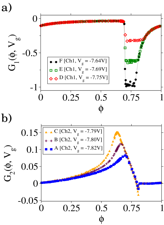
Figure 12: (Color online) PRCs $G_{1}(\phi,V_{g})$ and $G_{2}(\phi,V_{g})$ of electrical oscillator obtained by stimulating (a) $Ch_{1}$, and (b) $Ch_{2}$, which show responses of oscillators that desynchronize and synchronize, respectively, upon receiving common impulses. Each curve is labeled with a letter (A, B, C, $\cdots$) that corresponds to a location where impulse was applied ($Ch_{1}$ or $Ch_{2}$), and the MOSFET gate voltage creating the impulse, which corresponds to the Poisson mark $c$.

As in the simulation, we obtained the PRC experimentally by applying impulsive stimulus to the circuit. We varied the PRC characteristics by varying the location of the circuit to which impulses were applied. Figure 12 shows the experimental PRCs $G_{1}(\phi,V_{g})$ and $G_{2}(\phi,V_{g})$ obtained by stimulating $Ch1$ and $Ch2$ for several impulse intensities. Qualitatively different PRCs were obtained when we stimulated different locations. In contrast, varying the stimulus intensity to the same location resulted in similar but systematically different PRCs.

An experimental measurement has many sources of noise, which seriously degrades the first derivative calculated from a discretely sampled PRC, which is necessary in calculating the Lyapunov exponent. Assuming that the fluctuations seen in the derivative of the PRC are due to experimental noise and that the underlying response of the system is smoothly changing with respect to phase, we must infer the underlying smooth response from our noisy data.

To this end, we smoothed the PRC using a non-Gaussian Kalman filter Kitagawa based on a Markov state space model with a transition probability distribution given by the Cauchy distribution. The Kalman filter iteratively finds the ”true” values, $\{\bar{\phi}_{1},\bar{\phi}_{2},\cdots,\bar{\phi}_{N}\}$, at each $i$ of the data given the observed data $\{\phi_{1},\phi_{2},\cdots,\phi_{N}\}$ such that conditional probability

$$p(\{\bar{\phi}_{i}\}|\{\phi_{i}\},\{\mbox{filter parameters}\}),$$ (36)

is maximized. The method may be combined with Bayesian methods such as the Expectation-Maximization algorithm to choose the best filter parameters. We did not perform this step, but chose parameters that preserved the global shape of the PRC while yielding a smooth first derivative. This smoothed PRC was then used in Eq. (26) to calculate the Lyapunov exponent.

IV.3 Synchronization and desynchronization

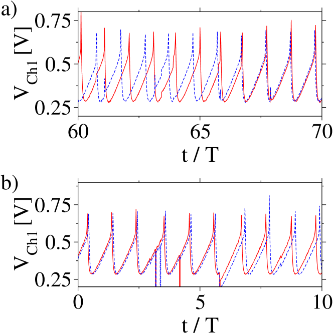
Figure 13: (Color online) Representative waveforms of electrical oscillators undergoing common-impulse induced synchronization ($V_{g}=-7.79$V added to $Ch_{2}$) (a) and desynchronization ($V_{g}=-7.69$V added to $Ch_{1}$) (b) measured at $Ch_{1}$. The Poisson impulse rate is $\lambda=1/4T$. Voltages traces in (b) actually extend below $0.2$V, but have been clipped to show detail.

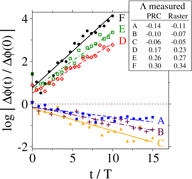
Figure 15: (Color online) Growth times of perturbations to electrical oscillator, where (A, B, C, $\cdots$, $F$) correspond to that introduced in Fig. 12. Data was taken for 80-150 trials, each with an ensemble of 20 oscillators, with Poisson impulse rate $\lambda=1/4T$. A comparison of the Lyapunov exponent with theory is shown in the table.

Figure 13 shows the voltage traces at $Ch_{1}$ for several different trials showing electrical oscillators synchronizing and desynchronizing due to common impulses. The PRC obtained when impulses were applied to $Ch_{1}$, Fig. 12(a), had a large jump, and the effect of the common impulse was predominantly a desynchronizing one. We were able to detect a synchronization-desynchronization transition in $Ch_{1}$ by varying the impulse intensity (data not shown), but because the synchronizing effects were relatively weak, we chose instead to investigate the synchronization due to impulses applied to $Ch_{2}$, where the PRC is smooth as shown in Fig. 12(b) so that we were able to observe common-impulse induced synchronization clearly, as shown in Fig. 14(a). We verified the theoretical predictions by measuring the Lyapunov exponent using the two methods outlined in the previous section. The results of the two methods of measurement of the Lyapunov exponent are summarized in the caption of Fig. 15. Considering the frequency drift among trials, the agreement between the results of the two methods seems reasonable. .

Note that our electrical limit-cycle oscillator is not near the bifurcation point and the PRC is not jagged in contrast to the FHN oscillator, even though the oscillators are desynchronized when impulses are applied. Therefore, the desynchronization effect is rather gradual, as shown in the raster plot, Fig. 14(b), which is qualitatively similar to the situation with strong impulses on the Stuart-Landau oscillators that we discuss in Appendix E.

V Summary

Through theoretical analysis, numerical simulations, and circuit experiments, we have demonstrated that phase synchronization, desynchronization, and clustering can be realized in a system of identical, uncoupled oscillators acted on by common Poisson impulses by changing the parameters of each individual oscillator, and also by varying the strength of the common impulse. We have clarified that once the phase response curves of the oscillator is known, such phase coherence phenomena can be quantitatively understood in a unified way. The desynchronization is an effect of the finite size of impulses that we use, in sharp contrast to the exclusively synchronizing effects that infinitesimal perturbations have.

It is quite remarkable that the synchronization and desynchronization of an ensemble of oscillators may be controlled in this way through a random signal. Depending on the oscillator characteristics, we could alter the coherence properties of the ensemble simply by changing the intensity of external random impulses. This approach would have potential applications in which it is desirable to change the global coherence properties of a network of oscillators. Applying common impulse of suitable intensity, it would be possible to effectively ”switch off” or ”switch on” the synchronization without changing the oscillator characteristics or modifying the coupling strength.

In this paper, we characterized the local stability of the synchronized states by a Lyapunov analysis, but not the global stability. In Ref. Nakao-Arai-Kawamura , we have presented a global stability analysis of the system for common Gaussian-white driving using an averaging technique for nonlinear oscillators. Similar formulation is also possible for the present common impulsive driving. The clustering phenomenon was realized only numerically for the FHN system, because our present experimental circuit does not appear to have a symmetric limit cycle or PRC compatible with clustering. Other limit-cycle electric oscillators with nearly symmetric limit cycles do exist, and investigation of clustering with such systems is now under progress. We expect that on-off intermittency and switching can also be observed in such electric oscillators. Detailed analysis on these topics will be reported in the future.

VI Acknowledgments

The authors wish to thank Y. Kuramoto for helpful discussions, especially suggesting us to analyze the impulse-driven case, and H. Fujisaka for all his insightful comments and advice. We also thank K. Aihara, A. Uchida, K. Yoshimura, H. Suetani, T. Shimokawa, J. Teramae, D. Tanaka, T. Kobayashi, Y. Kawamura and Y. Tsubo for various useful comments and information. This work is supported partially by the Grant-in-Aid for the 21st Century COE ”Center for Diversity and Universality in Physics”, and partially by the Grant-in-Aid for Young Scientists (B), 19760253, 2007, from the Ministry of Education, Culture, Sports, Science, and Technology of Japan.

Appendix A Poisson-driven Markov process (Jump process)

In this paper, we model the process of an oscillator receiving impulses as a Poisson-driven Markov process, or jump process Snyder ; Hanson . A general stochastic process $\bm{X}(t)$ driven by Poisson random impulses,

$$\dot{\bm{X}}(t)=\bm{F}(\bm{X})+\sum_{n=1}^{N(t)}\bm{G}(\bm{X},\bm{c}_{n})h(t-t_{n})$$ (37)

with point-like impulses $h(t)$ should be interpreted in the Ito picture as

$$\bm{X}(t)=\bm{X}(0)+\int_{0}^{t}\bm{F}(\bm{X}(s))ds+\sum_{n=1}^{N(t)}\bm{G}(\bm{X}(t_{n}-0),\bm{c}_{n}),$$ (38)

which is described as an integral equation of the form

$$\bm{X}(t)=\bm{X}(0)+\int_{0}^{t}\bm{F}(\bm{X}(s))ds+\int_{0}^{t}\int_{\bm{c}}\bm{G}(\bm{X}(s),\bm{c})M(dt,d\bm{c}),$$ (39)

or as a jump stochastic differential equation (SDE),

$$d\bm{X}(t)=\bm{F}(\bm{X})dt+\int_{\bm{c}}\bm{G}(\bm{X},\bm{c})M(dt,d\bm{c}).$$ (40)

Here, $M(dt,d\bm{c})$ represents a Poisson random measure Snyder ; Hanson , which gives the number of incident points during $[t,t+dt]$ having mark (jump magnitude) in $[\bm{c},\bm{c}+d\bm{c}]$, and $N(t)=\int_{0}^{t}\int_{\bm{c}}M(dt,d{\bm{c}})$ is the number of incident points during $[0,t]$. As usual in Ito-type stochastic differential equations, functions of ${\bm{X}}(t)$ and the Poisson random measure $M(dt,d\bm{c})$ at the same instant of time are independent. The expectation of $M(dt,d\bm{c})$ is

$$\langle M(dt,d\bm{c})\rangle=\lambda dtp(\bm{c})d\bm{c},$$ (41)

where $\lambda$ is the rate of the Poisson process and the marks are distributed as $p(\bm{c})$. Similarly, the covariance of $M(dt_{1},d\bm{c}_{1})$ and $M(dt_{2},d\bm{c}_{2})$ is Snyder ; Hanson

$$\mbox{Cov}[M(dt_{1},d\bm{c}_{1}),M(dt_{2},d\bm{c}_{2})]=\lambda\delta(t_{2}-t_{1})dt_{1}dt_{2}p(\bm{c}_{1})\delta(\bm{c}_{1}-\bm{c}_{2})d\bm{c}_{1}d\bm{c}_{2}.$$ (42)

As in the case of Wiener-driven Ito stochastic differential equations, we need to use a special rule in calculating the differential of a transformed process. A transformed process $V(t)=V(\bm{X}(t))$ obeys a jump SDE of the form

$$dV(t)=\left[\mbox{grad}_{\bm{X}}V(\bm{X})\cdot\bm{F}(\bm{X})\right]dt+\int_{\bm{c}}[V(\bm{X}+\bm{G}(\bm{X},\bm{c}))-V(\bm{X})]M(dt,d\bm{c}),$$ (43)

which is a stochastic chain rule for the jump process. The chain rule changes an additive process into a multiplicative process, just as in the case of white-Gaussian driven Markov processes.

Appendix B Single oscillator phase distribution

In the calculation of the Lyapunov exponent, we simplified the calculation by assuming that a single oscillator receiving random Poisson impulses is evenly distributed in phase when averaged over a long period of time. This is strictly not the case, as can be seen from the map $\phi(\theta)=\theta+G(\theta,{\bm{c}})$. It is obvious that certain values of $\phi(\theta)$ are arrived at more often than other values, because $G(\theta,\bm{c})$ is generally a nonlinear function of $\theta$. For completeness, we calculate the deviation from a flat phase PDF by the forward Kolmogorov equation Hanson . To this end, we define $\eta(\phi,{\bm{c}})=G(\theta,{\bm{c}})$, which is the jump as a function of the destination coordinate $\phi$. Then the probability density $p(\phi,t)$ of $\phi$ obeys

$$\frac{\partial}{\partial t}p(\phi,t)=-\frac{\partial}{\partial\phi}[\omega p(\phi,t)]-\lambda p(\phi,t)+\lambda\int_{\bm{c}}p({\bm{c}})p(\phi-\eta(\phi,{\bm{c}}))\left|1-\frac{\partial}{\partial\phi}\eta(\phi,{\bm{c}})\right|d{\bm{c}}.$$ (44)

We find the stationary PDF by setting $\partial p(\phi,t)/\partial t=0$. It is clear that the combination $\epsilon=\lambda/\omega$ determines the effect of the impulses, which is a small parameter from our initial assumption (the rate of the Poisson process $\lambda$ is small). We thus expand $p(\phi)$ in powers of $\epsilon$ away from the stationary PDF as $p(\phi)=1+\epsilon p_{1}(\phi)+\cdots$. Substituting this into the forward Kolmogorov equation, the first non-vanishing terms are of order $O(\epsilon^{1})$:

$$0=\frac{\partial}{\partial\phi}p_{1}(\phi)+1-\int_{\bm{c}}p({\bm{c}})\left|1-\frac{\partial}{\partial\phi}\eta(\phi,{\bm{c}})\right|d{\bm{c}}.$$ (45)

If the PRC does not change too rapidly, $-1<{\partial\eta(\phi,{\bm{c}})}/{\partial\phi}<1$, and the absolute value of the integrand may be removed, yielding

$$\frac{\partial}{\partial\phi}p_{1}(\phi)=-\int_{\bm{c}}p({\bm{c}})\frac{\partial}{\partial\phi}\eta(\phi,{\bm{c}})d{\bm{c}}.$$ (46)

Then

$$p_{1}(\phi)=\mbox{C}-\int_{\bm{c}}p({\bm{c}})\eta(\phi,{\bm{c}})d{\bm{c}}.$$ (47)

Since the integral of $p(\phi)$ over one period of the $O(\epsilon^{0})$ term is $1$ due to normalization, higher order terms $p_{1}(\phi),p_{2}(\phi),\cdots$ must vanish upon integration over a full period. Specifically, the $\int_{0}^{1}p_{1}(\phi)d\phi=0$ condition yields

$$C=\int_{\bm{c}}p({\bm{c}})\overline{\eta}({\bm{c}})d\bm{c}$$ (48)

where

$$\overline{\eta}({\bm{c}})=\int_{0}^{1}\eta(\phi,{\bm{c}})d\phi.$$ (49)

Therefore, we have for the first order approximation to the stationary phase PDF,

$$p(\phi)=1+\epsilon\int_{\bm{c}}\left[\overline{\eta}({\bm{c}})-\eta(\phi,{\bm{c}})\right]p({\bm{c}})d{\bm{c}}+O(\epsilon^{2}).$$ (50)

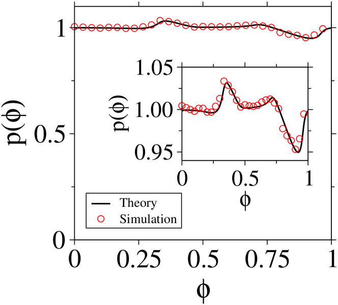
Figure 17: (Color online) The stationary phase distribution of a FitzHugh-Nagumo oscillator receiving random Poisson impulses, $I_{0}=0.8$, $c=0.5$ and $\lambda=1/4T$, calculated using a perturbation expansion of the forward Kolmogorov equation and by direct numerical simulation.

As we see from Fig. 17, $p(\phi)$ is close to constant as long as the parameter $\epsilon$ is small. In Ref. Nakao-Arai , we argued that for Poisson impulses, the lowest order correction to the uniform phase density does not contribute to the Lyapunov exponent based on a perturbation expansion of a Frobenius-Perron-type equation. Here we only point out that the correction to the uniform density is of $O(\lambda/\omega)$, which is small if the Poisson rate $\lambda$ is sufficiently smaller than the oscillator natural frequency $\omega$.

Appendix C Geometric Interpretation of the Synchronizing Mechanism

Weak impulses always synchronize uncoupled oscillators. Here we show through a simple Floquet analysis that this synchronization is a consequence of the stability of the limit cycle against weak perturbations. The generic oscillator under consideration in this article is described by an ordinary differential equation of the form

$$\dot{\bm{X}}(t)=\bm{F}(\bm{X}),$$ (51)

with a stable limit-cycle solution $\bm{X}_{0}(t)$ with period $T$. Linearizing Eq. (51) with respect to a small perturbation $\bm{u}(t)$ from the limit cycle, we obtain

$$\dot{\bm{u}}(t)=\bm{DF}(\bm{X})|_{\bm{X}=\bm{X}_{0}(t)}\bm{u}$$ (52)

where $\bm{DF}(\bm{X})|_{\bm{X}=\bm{X}_{0}(t)}$ is a periodic $M\times M$ Jacobian matrix. Ordinary differential equations of this form with periodic coefficients have solutions of the form $\bm{u}(t)=\bm{Q}(t)e^{\bm{R}t}\bm{u}(0)$ where $\bm{R}$ is a constant $M\times M$ matrix, and $\bm{Q}(t)=\bm{Q}(t+T)$ is a $T$-periodic $M\times M$ matrix. Since $\bm{Q}$ is periodic, we have $\bm{u}(T)=e^{\bm{R}T}\bm{u}(0)$. There is a corresponding value of the constant matrix $\bm{R}$ for each point on the limit cycle. The eigenvalues and eigenvectors of $e^{\bm{R}T}$, $\{\lambda_{i}\}$ and $\{\bm{e}_{i}\}$ respectively, have the property that $\bm{e}_{1}$ is in the direction along the limit cycle, $\lambda_{1}=1$ and $|\lambda_{i}|<1$ for $i\in\{2,\cdots,M\}$. The eigenvectors are known as the Floquet eigenvectors, and each point on the limit cycle has its own set of Floquet eigenvalues and eigenvectors.

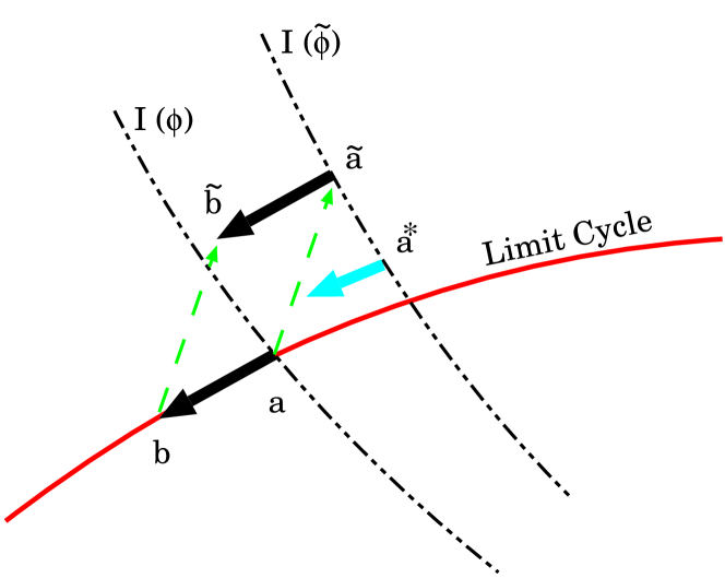
Figure 16: (Color online) Schematic of evolution two nearby orbits. $a=\bm{X}_{0}(\phi)$ and $b=\bm{X}_{0}(\phi)+\bm{z}(0)$ represent the spatial points at which 2 orbits receive a common additive impulse $\bm{c}$ on the limit cycle. The oscillators jump to $\tilde{a}=\bm{X}_{0}(\phi)+\bm{c}$ and $\tilde{b}=\bm{X}_{0}(\phi)+\bm{z}(0)+\bm{c}$. After the oscillator completes one period of unperturbed motion, through analysis of the Floquet eigenvectors and eigenvalues, we see that the difference vector has shrunk, i.e. $\left|\bm{z}(T)\right|<\left|\bm{z}(0)\right|$.

Figure 16 shows two infinitesimally separated orbits, 1 and 2, on the limit cycle at $a$, $\bm{X}_{0}(\phi)$, and $b$, $\bm{X}_{0}(\phi)+\bm{z}(0)$, with a phase $\phi$ isochron passing through $a$. Now let the two oscillators receive a common additive impulse $\bm{c}$ at $t=0$. The two oscillators jump discontinuously to $\tilde{a}$ at $\bm{X}_{0}(\phi)+\bm{c}$ and $\tilde{b}$ at $\bm{X}_{0}(\phi)+\bm{z}(0)+\bm{c}$, with a phase $\tilde{\phi}$ isochron passes through $\tilde{a}$. The set of Floquet eigenvalues and eigenvectors at $\phi$ and $\tilde{\phi}$ are $(\{\lambda_{i}\},\{\bm{e}_{i}\})$ and $(\{\tilde{\lambda}_{i}\},\{\tilde{\bm{e}}_{i}\})$, respectively. Since the impulse is additive, $\stackrel{{\scriptstyle\rightarrow}}{{ab}}=\stackrel{{\scriptstyle\rightarrow}}{{\tilde{a}\tilde{b}}}=\bm{z}(0)$. Expanding the difference vector $\bm{z}(0)$ by the Floquet vectors, we obtain $\bm{z}(0)=a_{1}\bm{e}_{1}=\sum_{i}\tilde{a}_{i}\tilde{\bm{e}}_{i}$. It is then obvious that $|a_{1}|>|\tilde{a}_{1}|$.

If the oscillator continues unperturbed for one period, the oscillator that received the impulse at $a$ at $t=0$ will now be at $a^{*}$, and $\bm{z}(T)\cong e^{\bm{R}T}\bm{z}(0)=\sum_{i}\tilde{\lambda}_{i}\tilde{a}_{i}\tilde{\bm{e}}_{i}$. Since $\left|\tilde{\lambda}_{i}\right|<1$ for $i\in\{2,\cdots,M\}$ from the stability of limit cycles, all components of $\bm{z}(T)$ with $i\geq 2$ will shrink, leaving only the first component along the limit cycle. We thus see that $|\bm{z}(T)|<|\bm{z}(0)|$ by virtue of $|\tilde{a}_{1}|<|a_{1}|$, namely that the application of a common impulse always shrinks the small separation between two orbits.

Appendix D Diffusion limit

We here derive the diffusion (Gaussian-white) limit of the impulse-driven oscillators for weak and frequent impulses. In taking the diffusion limit, we see that common impulse always results in the synchronization of oscillators since the Lyapunov exponent is bounded above by 0, and we see that desynchronization can only be understood by analyzing finite-magnitude perturbations to the limit cycle orbit.

D.1 Diffusion limit

We have until now considered finite Poisson impulses whose inter-impulse times are much longer than the natural period of the oscillators. The condition for the phase reduction is also satisfied by setting the combination of impulse intensity and the Poisson rate appropriately small, so that we may also consider a situation where the effect of Poisson impulses become infinitesimal but with inter-impulse times that are much faster than the natural time scales of the oscillators. Specifically, we consider the limit $\lambda\to\infty$ and the effect of impulses $\sigma_{k}\to 0$ such that $\lambda\langle\sigma_{k}\sigma_{l}\rangle_{\bm{c}}$ is kept constant and higher order terms like $\lambda\langle\sigma_{k}\sigma_{l}\sigma_{m}\rangle$ vanish $(k,l,m=1,\cdots,M)$. To take this limit, it is necessary that the net effect of the impulses vanishes, namely,

$$\langle\sigma_{k}(\phi,\bm{c})\rangle_{\bm{c}}=\int_{\bm{c}}p(\bm{c})\sigma_{k}(\bm{X}_{0}(\phi),\bm{c})d\bm{c}=0,\;\;\;\;(k=1,\cdots,M),$$ (53)

where we introduced the notation $\langle A(\phi,\bm{c})\rangle_{\bm{c}}=\int_{\bm{c}}A(\phi,\bm{c})p(\bm{c})d\bm{c}$ with fixed $\phi$. Under these conditions, we can consider the diffusion limit of a stochastic jump process.

The Kramers-Moyal expansion of the Chapman-Kolmogorov equation is Risken

$$\frac{\partial p(\phi,t)}{\partial t}=\sum_{n=1}^{\infty}\frac{1}{n!}\left(-\frac{\partial}{\partial\phi}\right)^{n}\left[K^{(n)}(\phi)p(\phi,t)\right],$$ (54)

where the Kramers-Moyal coefficient $K^{(n)}$ is given by

$$K^{(n)}(\phi)=\lim_{\Delta t\to 0}\frac{\langle\Delta\phi^{n}\rangle}{\Delta t}.$$ (55)

Here, $\Delta\phi$ is the jump within duration $\Delta t$ of the stochastic process starting from $\phi$, and the conditional average is taken over possible realizations of the stochastic process starting from $\phi$. If the coefficients higher than the second order vanish, we obtain a Fokker-Planck equation

$$\frac{\partial p(\phi,t)}{\partial t}=-\frac{\partial}{\partial\phi}\left[v(\phi)p(\phi,t)\right]+\frac{1}{2}\frac{\partial^{2}}{\partial\phi^{2}}\left[D(\phi)p(\phi,t)\right]$$ (56)

for the Wiener-driven Markov process, whose drift $v(\phi)$ and diffusion coefficient $D(\phi)$ are given by

$$v(\phi)=K^{(1)}(\phi),\;\;\;\;\;D(\phi)=K^{(2)}(\phi).$$ (57)

We now find $\langle\Delta\phi\rangle$ and $\langle\Delta\phi^{2}\rangle$ for a jump process, where the expectation is to be taken with fixed $\phi$. Starting with Eq. (8),

$$\langle\Delta\phi\rangle = \omega\Delta t+\int_{0}^{\Delta t}\int_{\bm{c}}G(\phi,\bm{c})\langle M(dt,d\bm{c})\rangle+O(\Delta t^{2})$$ (58)

$$= \omega\Delta t+\lambda\Delta t\langle G(\phi,\bm{c})\rangle_{\bm{c}}+O(\Delta t^{2}).$$ (60)

Similarly,

$$\langle\Delta\phi^{2}\rangle = \langle(\Delta\phi-\langle\Delta\phi\rangle)^{2}\rangle+O(\Delta t^{2})$$ (61)

$$= \int_{0}^{\Delta t}\int_{0}^{\Delta t}\int_{\bm{c}}\int_{\bm{c}^{\prime}}G(\phi,\bm{c})G(\phi^{\prime},\bm{c}^{\prime})\;\mbox{Cov}\left[M(dt,\bm{c}),M(dt^{\prime},\bm{c}^{\prime})\right]+O(\Delta t^{2})$$ (63)

$$= \lambda\Delta t\langle G(\phi,\bm{c})^{2}\rangle_{\bm{c}}+O(\Delta t^{2}).$$ (65)

It can be checked that $\langle\Delta\phi^{3}\rangle$ and higher-order moments vanish by taking the diffusion limit, so that they can be dropped. The Kramers-Moyal coefficients are given by

$$K^{(1)}(\phi)=\omega+\langle G(\phi,{\bm{c}})\rangle_{\bm{c}},\;\;\;\;\;K^{(2)}(\phi)=\langle G(\phi,{\bm{c}})^{2}\rangle_{\bm{c}},\;\;\;\;\;K^{(n)}(\phi)=0\;\;(n\geq 3).$$ (66)

Hereafter, for simplicity, we may not explicitly indicate the dependence of the function $\bm{g}(\bm{X}_{0}(\phi),\bm{c})$, $\bm{\sigma}(\bm{X}_{0}(\phi))$, or $\bm{Z}(\phi)$ on $\phi$ and $\bm{c}$. To evaluate the $v(\phi)$ and $D(\phi)$, we must evaluate $\langle G(\phi,\bm{c})\rangle_{\bm{c}}$ and $\langle G(\phi,\bm{c})^{2}\rangle_{\bm{c}}$. Since we assume the effect of impulses $\bm{g}$ to be small, we first rewrite $G(\phi,\bm{c})$ by Taylor expanding,

$$G(\phi,\bm{c}) = \phi\bigl{(}\bm{X}_{0}(\phi)+\bm{g}(\bm{X}_{0}(\phi),\bm{c})\bigr{)}-\phi$$ (67)

$$= \sum_{k=1}^{M}\left.\frac{\partial\phi}{\partial X_{k}}\right|_{\bm{X}=\bm{X}_{0}(\phi)}g_{k}+\frac{1}{2}\sum_{k=1}^{M}\sum_{l=1}^{M}\left.\frac{\partial^{2}\phi}{\partial X_{k}\partial X_{l}}\right|_{\bm{X}=\bm{X}_{0}(\phi)}g_{k}g_{l}+\cdots.$$ (69)

¿From the definition of the phase sensitivity function, Eq. (13), we obtain

$$\left.\frac{\partial\phi}{\partial X_{k}}\right|_{\bm{X}=\bm{X}_{0}(\phi)}=Z_{k}(\phi),$$ (70)

and

$$\left.\frac{\partial^{2}\phi}{\partial X_{k}\partial X_{l}}\right|_{\bm{X}=\bm{X}_{0}(\phi)}=\left.\frac{\partial Z_{l}}{\partial X_{k}}\right|_{\bm{X}=\bm{X}_{0}(\phi)}=\frac{dZ_{l}}{d\phi}\left.\frac{\partial\phi}{\partial X_{k}}\right|_{\bm{X}=\bm{X}_{0}(\phi)}=Z_{k}(\phi)Z_{l}^{\prime}(\phi).$$ (71)

Keeping only terms up to second order in $\bm{g}$, we obtain

$$\langle G(\phi,\bm{c})\rangle_{\bm{c}} = \sum_{k}Z_{k}\langle g_{k}\rangle_{\bm{c}}+\frac{1}{2}\sum_{k,l}Z_{k}Z_{l}^{\prime}\langle g_{k}g_{l}\rangle_{\bm{c}},$$ (72)

$$\langle G(\phi,\bm{c})^{2}\rangle_{\bm{c}} = \sum_{k,l}Z_{k}Z_{l}\langle g_{k}g_{l}\rangle_{\bm{c}}.$$ (74)

Depending on the picture of the original Eq. (1), the approximate jump magnitude $\bm{g}(\bm{X}_{0}(\phi),\bm{c})$ for a given mark $\bm{c}$ is

$$\bm{g}(\bm{X}_{0}(\phi),\bm{c})=\left\{\begin{array}[]{ll}\bm{\sigma}(\bm{X}_{0}(\phi),\bm{c})&\hskip 2.84526pt\mbox{(Ito)},\cr\cr\left.\left(e^{\hat{D}}-1\right)\bm{X}\right|_{\bm{X}=\bm{X}_{0}(\phi)}&\hskip 2.84526pt\mbox{(Stratonovich)}.\end{array}\right.$$ (75)

For $v(\phi)$ and $D(\phi)$ in the Ito picture of Eq. (1), we obtain

$$v(\phi) \cong \omega+\frac{\lambda}{2}\sum_{k,l}Z_{k}Z_{l}^{\prime}\langle\sigma_{k}\sigma_{l}\rangle_{\bm{c}},$$ (76)

$$D(\phi) \cong \sum_{k,l}Z_{k}Z_{l}\langle\sigma_{k}\sigma_{l}\rangle_{\bm{c}},$$ (78)

where we utilized the assumption $\langle\sigma_{k}(\phi,\bm{c})\rangle_{\bm{c}}=\int_{\bm{c}}p(\bm{c})\sigma_{k}(\bm{X}_{0}(\phi),\bm{c})d\bm{c}=0$. For $v(\phi)$ and $D(\phi)$ corresponding to the Stratonovich picture of Eq. (1), we obtain up to $O(\sigma_{k}\sigma_{l})$,

$$g_{k}(\bm{X}_{0}(\phi),\bm{c}) \cong \hat{D}X_{k}|_{\bm{X}=\bm{X}_{0}(\phi)}+\frac{1}{2}\hat{D}^{2}X_{k}|_{\bm{X}=\bm{X}_{0}(\phi)}\cong\sigma_{k}+\frac{1}{2}\sum_{l}\sigma_{l}\frac{\partial\sigma_{k}}{\partial X_{l}},$$ (79)

$$g_{k}(\bm{X}_{0}(\phi),\bm{c})g_{l}(\bm{X}_{0}(\phi),\bm{c}) \cong \sigma_{k}\sigma_{l},$$ (80)

so in the Stratonovich picture of Eq. (1), we obtain

$$v(\phi) \cong \omega+\frac{\lambda}{2}\sum_{k,l}\left(Z_{k}Z_{l}^{\prime}\langle\sigma_{k}\sigma_{l}\rangle_{\bm{c}}+Z_{k}Z_{l}\langle\sigma_{k}^{\prime}\sigma_{l}\rangle_{\bm{c}}\right),$$ (81)

$$D(\phi) \cong \sum_{k,l}Z_{k}Z_{l}\langle\sigma_{k}\sigma_{l}\rangle_{\bm{c}},$$ (83)

where we used

$$\sigma_{l}\frac{\partial\sigma_{k}}{\partial X_{l}}=\sigma_{l}\frac{\partial\sigma_{k}}{\partial\phi}\frac{\partial\phi}{\partial X_{l}}=\sigma_{l}Z_{l}\frac{\partial\sigma_{k}}{\partial\phi}.$$ (84)

Now that we have $v(\phi)$ and $D(\phi)$ for both cases, we write an FPE, and find the corresponding Ito SDE. The Ito SDE corresponding to the Ito picture, Eq. (4), reads

$$d\phi(t) = \left(\omega+\frac{\lambda}{2}\sum_{k,l}Z_{k}Z_{l}^{\prime}\langle\sigma_{k}\sigma_{l}\rangle_{\bm{c}}\right)dt+\sqrt{\lambda}\sum_{k,m}Z_{k}G_{km}dW_{m}(t),$$ (85)

where we introduced $M$ independent Wiener processes $\{dW_{m}(t)\}$ ($m=1,\cdots,M$) and an $M\times M$ coupling matrix $G_{km}(\phi)$ that satisfies

$$\sum_{m}G_{km}(\phi_{1})G_{lm}(\phi_{2})=\langle\sigma_{k}(\phi_{1})\sigma_{l}(\phi_{2})\rangle_{\bm{c}}.$$ (86)

Similarly, the Ito SDE corresponding to the Stratonovich picture, Eq.(6), leads to

$$d\phi(t) = \left[\omega+\frac{\lambda}{2}\sum_{k,l}\left(Z_{k}Z_{l}^{\prime}\langle\sigma_{k}\sigma_{l}\rangle_{\bm{c}}+Z_{k}Z_{l}\langle\sigma_{k}^{\prime}\sigma_{l}\rangle_{\bm{c}}\right)\right]dt+\sqrt{\lambda}\sum_{k,m}Z_{k}G_{km}dW_{m}(t).$$ (87)

Using the transformation rule between Ito SDE and Stratonovich SDE Gardiner ; Arnold , this equation can concisely be expressed as a Stratonovich SDE

$$\mbox{(S)}\;\;\;d\phi(t)=\omega dt+\sqrt{\lambda}\sum_{k,m}Z_{k}(\phi)G_{km}(\phi)dW_{m}(t),$$ (88)

which was the starting point of the previous works Teramae-Dan ; Nakao-Arai-Kawamura .

D.2 Linear stability of the synchronized state

In both pictures of Eq. (1), the diffusion-limit Ito SDE takes the form

$$d\phi(t)=\left[\omega+a(\phi)\right]dt+\sum_{m}b_{m}(\phi)dW_{m}(t),$$ (89)

where $a(\phi)$ is periodic in $\phi$, and $b_{m}(\phi)=\sqrt{\lambda}\sum_{k}Z_{k}(\phi)G_{km}(\phi)$. We are interested in the linearized dynamics of the small perturbation $\psi(t)$ to $\phi(t)$,

$$d\psi(t)=\left[a^{\prime}(\phi)dt+\sum_{m}b_{m}^{\prime}(\phi)dW_{m}(t)\right]\psi.$$ (90)

Using the Ito formula Gardiner ; Arnold for changing variables to $y=\log|\psi|$,

$$dy(t)=\left[a^{\prime}(\phi)-\frac{1}{2}\sum_{m}b_{m}^{\prime}(\phi)^{2}\right]dt+\sum_{m}b_{m}^{\prime}(\phi)dW_{m}(t).$$ (91)

The expectation is calculated by replacing the dynamics with the single-oscillator phase PDF, $p(\phi)=1$, so the Lyapunov exponent is given as

$$\Lambda=-\frac{1}{2}\int_{0}^{1}\sum_{m}b_{m}^{\prime}(\phi)^{2}d\phi\leq 0,$$ (92)

where the integral of $a^{\prime}(\phi)$ vanishes due to the periodicity of $a(\phi)$, and the noise term vanishes because $b_{m}^{\prime}(\phi)$ and $dW_{m}(t)$ are independent in the Ito SDE and the expectation of $dW_{m}(t)$ is $0$. Therefore, the Lyapunov exponent is the same no matter the picture of the SDE Eq. (7). Inserting $b_{m}(\phi)=\sqrt{\lambda}\sum_{k}Z_{k}(\phi)G_{km}(\phi)$, the summation in Eq. (92) can be calculated as

$$\sum_{m}b_{m}^{\prime 2} = \lambda\sum_{k,l}Z_{k}^{\prime}\left[\sum_{m}G_{km}G_{lm}\right]Z_{l}^{\prime}+\lambda\sum_{k,l}Z_{k}^{\prime}\left[\sum_{m}G_{km}G_{lm}^{\prime}\right]Z_{l}$$ (96)

$$+\lambda\sum_{k,l}Z_{k}\left[\sum_{m}G_{km}^{\prime}G_{lm}\right]Z_{l}^{\prime}+\lambda\sum_{k,l}Z_{k}\left[\sum_{m}G_{km}^{\prime}G_{lm}^{\prime}\right]Z_{l}$$

$$= \lambda\sum_{k,l}\left(Z_{k}^{\prime}\langle\sigma_{k}\sigma_{l}\rangle_{\bm{c}}Z_{l}^{\prime}+Z_{k}^{\prime}\langle\sigma_{k}\sigma_{l}^{\prime}\rangle_{\bm{c}}Z_{l}+Z_{k}\langle\sigma_{k}^{\prime}\sigma_{l}\rangle_{\bm{c}}Z_{l}^{\prime}+Z_{k}\langle\sigma_{k}^{\prime}\sigma_{l}^{\prime}\rangle_{\bm{c}}Z_{l}\right),$$ (99)

where we used

$$\langle\sigma_{k}^{\prime}\sigma_{l}\rangle_{\bm{c}}(\phi)=\left.\frac{\partial}{\partial\phi_{1}}\langle\sigma_{k}(\phi_{1})\sigma_{l}(\phi_{2})\rangle_{\bm{c}}\right|_{(\phi_{1},\phi_{2})=(\phi,\phi)},$$ (100)

etc., so we finally obtain

$$\Lambda=-\frac{\lambda}{2}\sum_{k,l}\int_{0}^{1}\left[Z_{k}^{\prime}Z_{l}^{\prime}\langle\sigma_{k}\sigma_{l}\rangle_{\bm{c}}+2Z_{k}^{\prime}Z_{l}\langle\sigma_{k}\sigma_{l}^{\prime}\rangle_{\bm{c}}+Z_{k}Z_{l}\langle\sigma_{k}^{\prime}\sigma_{l}^{\prime}\rangle_{\bm{c}}\right].$$ (101)

This expression coincides with the approximate Lyapunov exponent that we obtained by a Taylor expansion in Eq. (28), and gives a multiplicative generalization to the previous results obtained by Teramae and Tanaka in Ref. Teramae-Dan (our result in Ref. Nakao-Arai-Kawamura includes this result).

Appendix E Stuart-Landau oscillator

In Sec. III, we discussed the case in which the response of the oscillator to sufficiently strong perturbations result in PRCs that appear jagged, Fig. 4b). For such PRCs, the desynchronization is intuitive: if a nearly-synchronized group of oscillators near such a jagged response receive an common impulse, they end up with widely distributed phases Nagai-Nakao ; Nakao-Arai . In Ref. Goldobin-Pikovsky , the same situation is described differently, where the importance of the ”heavy-tails” of the distribution of relaxation rates of transverse perturbations for oscillators near the bifurcation point is emphasized.

However, the PRC need not have such a pathologic shape for desynchronization. It may even be sinusoidal as shown in Ref. Pikovsky-R-K1 , Sec. 15. Such a case occurs with the Stuart-Landau (SL) oscillator, which describes the small-amplitude oscillations near the supercritical Hopf bifurcation point of a general system of ODEs Kuramoto .

Consider the following SL oscillator driven by random Poisson impulses:

$$\dot{u} = (u-c_{0}v)-(u-c_{2}v)(u^{2}+v^{2})+\sigma(v,c)\sum_{n=1}^{N(t)}h(t-t_{n})$$

$$\dot{v} = (v+c_{0}u)-(v+c_{2}u)(u^{2}+v^{2}),$$ (102)

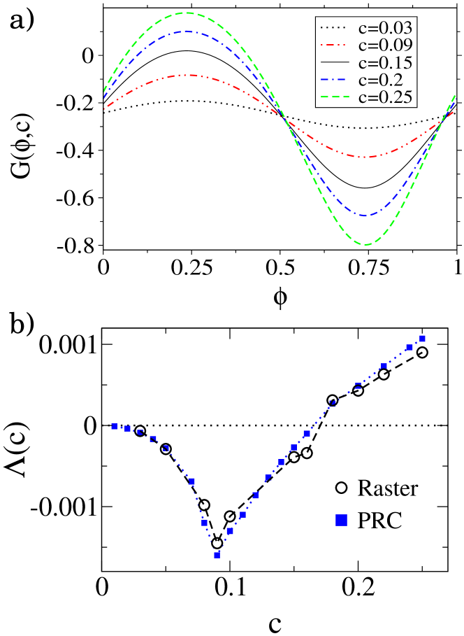
Figure 18: (Color online) a) PRCs for SL model ($c_{0}=-c_{2}=12$) for various additive impulse intensities. b) Comparison of the Lyapunov exponents $\Lambda$ between the direct measurement from the raster plot and the theoretical prediction from the PRC for SL oscillators driven by additive impulses of intensity $c$, and Poisson impulse rate $\lambda=1/380T$. We chose a large inter-impulse interval (380T) because the SL oscillators have a very slow relaxation back to the limit-cycle orbit following a perturbation.

where $h(t)$ and $\sigma(v,c)$ as described above for the FHN oscillator. For comparison with the FHN oscillator, we followed the same procedure for the SL oscillators and found the existence of synchronizing and desynchronizing impulse strengths (raster data not shown but are qualitatively similar to Fig. 2). PRCs are shown in Fig. 18(a) and Lyapunov exponents obtained using Eq. (26) and by direct measurement are shown in Fig. 18(b). The PRCs are almost sinusoidal but slightly deformed because the impulse intensity $c$ is finite. As expected, the Lyapunov exponent $\Lambda(c)$ shown in Fig. 18(b) is qualitatively very similar to that obtained in Ref. Pikovsky-R-K1 calculated for a circle map with a sinusoidal PRC receiving common Poisson impulses, which predicts synchronization for weak impulses and desynchronization for stronger impulses.

Note that in our present treatment of Poisson-driven limit cycles, we do not need to discuss the FHN-type oscillator and the SL-type oscillator separately. We can simply adopt the same one-dimensional phase model with the standard definition of the PRC, which quantitatively predicts the Lyapunov exponent in both synchronization and desynchronization regimes.

Figure 2: Raster plots of FHN oscillators showing synchronization and desynchronization due to common impulses with rate $\lambda=1/4T$ for both. Time axis normalized by natural frequency of oscillators. Each tick indicates the time oscillator passed through $\phi=0$ near the limit cycle. (a) Synchronization of FHN ($I_{0}=0.8$, $c=0.3$, $D=5\times 10^{-6}$) and (b) Desynchronization of FHN ($I_{0}=0.34$, $c=0.2$, $D=5\times 10^{-8}$). The wide blank without ticks in (b) corresponds to the situation where the orbit is transiently trapped around the unstable focus.

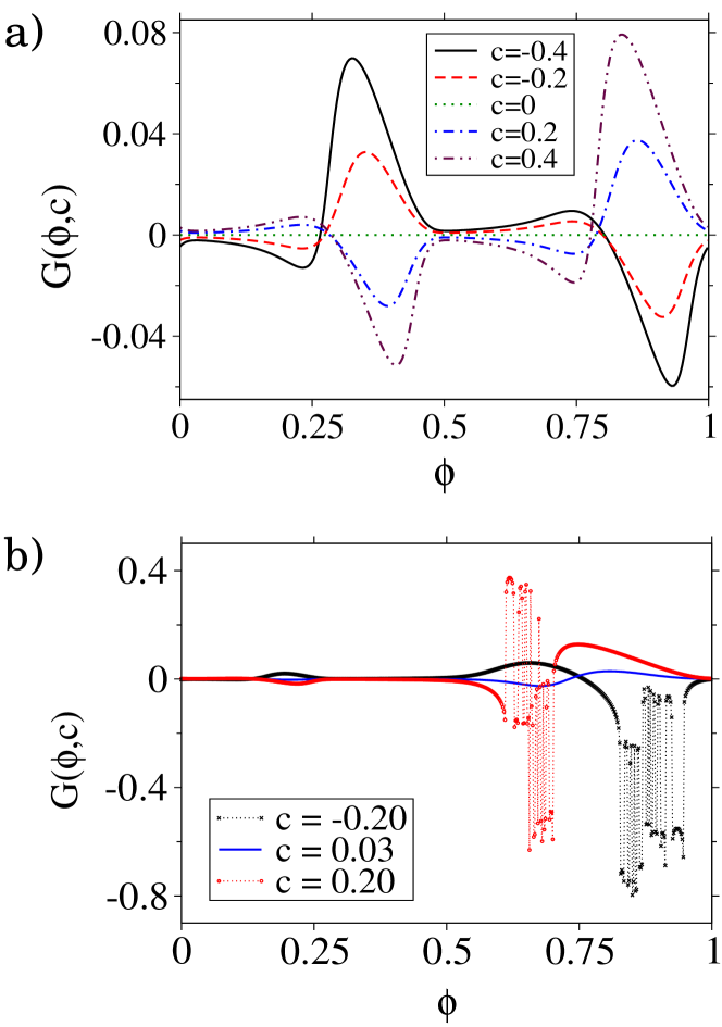
Figure 4: (Color online) (a) PRCs for FHN with $I_{0}=0.8$ and additive impulse intensities $c\in[-0.4,0.4]$, (b)PRCs for FHN with $I_{0}=0.34$ and additive impulse intensities $c=-0.20,0.03,0.20$.

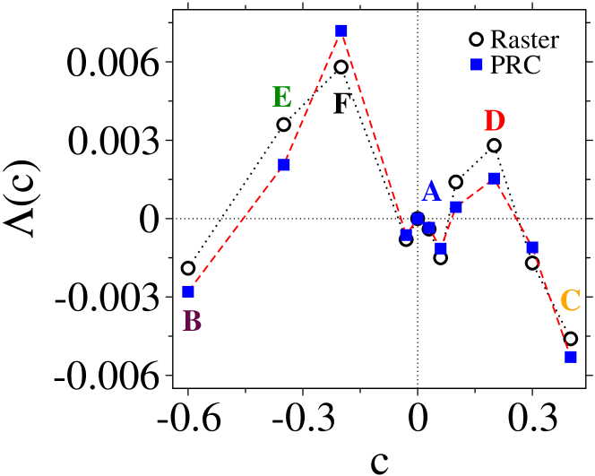
Figure 8: (Color online) Comparison of the Lyapunov exponents $\Lambda$ between the direct measurement from the raster plot and the theoretical prediction from the PRC for FHN with parameter $I_{0}=0.34$ and additive impulses with rate $\lambda=1/4T$. Labels A, B, $\cdots$, $F$ correspond to those in Fig. 6.

Figure 11: (a) Diagram of electrical circuit with limit-cycle behavior. Computer-generated impulses control $V_{g}$, which turns MOSFET $\mbox{M}_{1}$ current source on/off. Switch $\mbox{S}_{1}$ allows us to send common impulse to either $Ch_{1}$ or $Ch_{2}$. (b) Limit cycle of electrical circuit produce by measuring voltages at $Ch_{1}$ or $Ch_{2}$ as given in (a).

Figure 14: Raster plots of electrical oscillators showing synchronization and desynchronization. The Poisson impulse rate is $\lambda=1/4T$. Each tick indicates the time oscillator passed through $\phi=0$. (a) Synchronization of electrical oscillators (impulse added to $Ch_{2}$, $V_{g}=-7.79V$) and (b) Desynchronization of electrical oscillators (impulse added to $Ch_{1}$, $V_{g}=-7.64V$).

References

- (1) R. Roy and K.S. Thornburg, Jr., Phys. Rev. Lett. 72, 2009 (1994); A. Uchida, R. McAllister, and R. Roy, Phys. Rev. Lett. 93, 244102 (2004).
- (2) Z. F. Mainen and T. J. Sejnowski, Science 268, 1503 (1995).
- (3) M. D. Binder and R. K. Powers, J. Neurophysiol 86, 2266 (2001).
- (4) R. F. Galan, N. F. Trocme, G. B. Ermentrout, and N. N. Urban, J. Neurosci 26(14), 3646 (2006).
- (5) T. Royama, Analytical Population Dynamics (Chapman & Hall, New York, 1992)
- (6) R. Toral, C. R. Mirasso, E. Hernández-García, and O. Piro, Chaos 11, 665 (2001).
- (7) C. Zhou and J. Kurths, Phys. Rev. Lett., 88 230602 (2002)
- (8) K. Pakdaman, Neural Comput. 14 781, (2002).
- (9) A. Pikovsky, M. Rosenblum, and J. Kurths, Synchronization: A universal concept in nonlinear sciences, (Cambridge University Press, 2001).
- (10) J. Teramae and D. Tanaka, Phys. Rev. Lett. 93, 204103 (2004); Prog. Theoret. Phys. Suppl. 161, 360 (2006).
- (11) D. S. Goldobin and A. Pikovsky, Phys. Rev. E 71, 045201(R) (2005); Physica A 351, 126 (2005); Phys. Rev. E 73, 061906 (2006).
- (12) K. Nagai, H. Nakao, and Y. Tsubo, Phys. Rev. E 71, 036217 (2005); H. Nakao, K. Nagai, and K. Arai, Prog. Theoret. Phys. Suppl. 161, 294 (2006).
- (13) H. Nakao, K. Arai, K. Nagai, Y. Tsubo, and Y. Kuramoto, Phys. Rev. E 72, 026220 (2005).
- (14) H. Nakao, K. Arai and Y. Kawamura, Phys. Rev. Lett. 98, 184101 (2007).
- (15) K. K. Lin, E. Shea-Brown, and L.-S. Young, arXiv:0708.3061 (2007).
- (16) P. A. Tass, Phase Resetting in Medicine and Biology - Stochastic Modelling and Data Analysis (Springer, Berlin, 1999).
- (17) Y. Zhai, I. Z. Kiss, P. A. Tass, and J. L. Hudson, Phys. Rev. E 71, 065202(R) (2005).
- (18) A. T. Winfree, Nature 253 315 (1975).
- (19) H. Ukai, T. J. Kobayashi, M. Nagano, K. Masumoto, M. Sujino, T. Kondo, K. Yagita, Y. Shigeyoshi and H. R. Ueda, Nature Cell Biology 9 1327 (2007).
- (20) A. T. Winfree, The Geometry of Biological Time (Springer-Verlag, New York, 2001)
- (21) Y. Kuramoto, Chemical Oscillation, Waves, and Turbulence (Springer-Verlag, Tokyo, 1984) (republished by Dover, New York, 2003).
- (22) D. L. Snyder, Random Point Processes, (John Wiley & Sons, Inc. 1975).
- (23) F. B. Hanson, Applied Stochastic Processes and Control for Jump-Diffusions, SIAM Books, 2007.
- (24) E. Wong and M. Zakai, Int. J. Eng. Sci. 3, 213 (1965).
- (25) S. I. Marcus, IEEE Trans. on Information Theory, 24, 2, 164-172 (1978).
- (26) C. W. Gardiner, Handbook of Stochastic Methods for Physics, Chemistry and the Natural Sciences (Springer, 1997).
- (27) L. Arnold, Stochastic Differential Equations: Theory and Applications (John Wiley & Sons, 1973).
- (28) C. Koch, Biophysics of Computation (Oxford University Press, Oxford, 1999).
- (29) D. Hansel, G. Mato, and C. Meunier, Phys. Rev. E 48, 3470 (1993).
- (30) H. Fujisaka and T. Yamada, Prog. Theor. Phys., 69, 32 (1983); H. Fujisaka, Prog. Theor. Phys. 70, 1264 (1983); H. Fujisaka and T. Yamada, Prog. of Theor. Phys., 74, 918 (1985).
- (31) J.F. Heagy, N. Platt, and S.M. Hammel, Phys. Rev. E 49, 1140 (1994).
- (32) S. C. Venkataramani, T. M. Antonsen, Jr., E. Ott, and J. C. Sommerer, Physica (Amsterdam) 96D, 66 (1996);
- (33) M. Sauer and F. Kaiser, Phys. Rev. E 54, 2468 (1996).
- (34) F. Rödelsperger, A. Čenys, and H. Benner, Phys. Rev. Lett 75, 2594 (1995).
- (35) T. John, R. Stannarius, and U. Behn, Phys. Rev. Lett. 83, 749 (1999).
- (36) A. S. Pikovsky, Phys. Lett. A 165, 33 (1992).
- (37) G. Kitagawa and W. Gersch, Lecture Notes in Statistics: Smoothness Priors Analysis of Time Series (Springer, 1996).
- (38) K. Yoshida, K. Sato, A. Sugamaga, J. Sound and Vibration 290, 34 (2006).
- (39) R. F. Galan, G. B. Ermentrout and N. N. Urban, Phys. Rev. Lett. 94, 158101, (2005).
- (40) T. Tateno and H. P. C. Robinson, Biophysical Journal, 92, 683 (2007).
- (41) H. Risken, The Fokker-Planck Equation: Methods of Solution and Applications (Springer, 1996).
- (42) K. Yoshimura, P. Davis, and A. Uchida, arXiv:0705.4520 (2007).