Information Filtering via Self-Consistent Refinement

Abstract

Recommender systems are significant to help people deal with the world of information explosion and overload. In this Letter, we develop a general framework named self-consistent refinement and implement it be embedding two representative recommendation algorithms: similarity-based and spectrum-based methods. Numerical simulations on a benchmark data set demonstrate that the present method converges fast and can provide quite better performance than the standard methods.

Introduction.—The last few years have witnessed an explosion of information that the Internet and World Wide Web have brought us into a world of endless possibilities: people may choose from thousands of movies, millions of books, and billions of web pages. The amount of information is increasing more quickly than our processing ability, thus evaluating all these alternatives and then making choice becomes infeasible. As a consequence, an urgent problem is how to automatically extract the hidden information and do a personal recommendation. For example, Amazon.com uses one’s purchase record to recommend books Linden2003 , and AdaptiveInfo.com uses one’s reading history to recommend news Billsus2002 . Motivated by the significance in economy and society, the design of an efficient recommendation algorithm becomes a joint focus from engineering science Herlocker2004 ; Adomavicius2005 to marketing practice Ansari2000 ; Ying2006 , from mathematical analysis Kumar2001 ; Donovan2005 to physics community Maslov2001 ; Laureti2006 ; Zhang2007a ; Zhang2007b ; Zhou2007a ; Zhou2007b ; Yu2006 ; Blattner2007 .

A recommender system, consisted of $N$ users and $M$ items, can be fully described by an $N\times M$ rating matrix $R$, with $R_{i\alpha}\neq 0$ the rating user $i$ gives to item $\alpha$. If $i$ has not yet evaluated $\alpha$, $R_{i\alpha}$ is set as zero. The aim of a recommender system, or of a recommendation algorithm, is to predict ratings for the items have not been voted. To evaluate the algorithmic accuracy, the given data set is usually divided into two parts: one is the training set, and the other one is the testing set. Only the information contained in the training set can be used in the prediction. Denoting the predicted rating matrix as $\tilde{R}$, the most commonly used measurement for the algorithmic accuracy, namely the mean average error (MAE), is defined as:

$$\emph{MAE}=\frac{1}{S}\sum_{(i,\alpha)}|\tilde{R}_{i\alpha}-R^{*}_{i\alpha}|,$$ (1)

where the subscript $(i,\alpha)$ runs over all the elements corresponding to the non-zero ratings in testing set, $R^{*}$ denotes the rating matrix for testing set, and $S$ is the number of non-zero ratings in $R^{*}$.

Thus far, the most accurate algorithms are content-based Pazzani2007 . However, those methods are practical only if the items have well-defined attributes, and those attributes can be extracted automatically. Besides the content-based algorithms, the recommendation methods can be classified into two main categories: similarity-based Konstan1997 ; Sarwar2001 and spectrum-based Billsus1998 ; Sarwar2000 . In this Letter, we propose a generic framework of self-consistent refinement (SCR) for the personal recommendation, which is implemented by embedding the similarity-based and spectrum-based methods, respectively. Numerical simulations on a benchmark data set demonstrate the significant improvement of algorithmic performance via SCR compared with the standard methods.

Generic framework of SCR.—The similarity-based and spectrum-based algorithms, including their extensions, can be expressed in a generic matrix formula

$$\tilde{R}=\mathfrak{D}(R),$$ (2)

where $R$ is the rating matrix obtained from the training set, $\tilde{R}$ the predicted rating matrix, and $\mathfrak{D}$ a matrix operator. This operator, $\mathfrak{D}$, may be extremely simple as a left-multiplying matrix used in the basic similarity-based method, or very complicated, usually involving a latent optimization process, like the case of rank-$k$ singular value decomposition (see below for details). Most previous works concentrated on the design of the operator $\mathfrak{D}$. In contrast, we propose a completely new scenario where Eq. (2) is replaced by a SCR via iterations. Denoting the initial configuration $R^{(0)}=R$, and the initial time step $k=0$, a generic framework of SCR reads:

(i) Implement the operation $\mathfrak{D}(R^{(k)})$;

(ii) Set the elements of $R^{(k+1)}$ as

$$R_{i\alpha}^{(k+1)}=\left\{\begin{array}[]{cc}\mathfrak{D}(R^{(k)})_{i\alpha},&R_{i\alpha}=0,\\ R_{i\alpha},&R_{i\alpha}\neq 0.\end{array}\right.$$ (3)

Then, set $k=k+1$.

(iii) Repeat (i)(ii) until the difference between $R^{(k)}$ and $R^{(k-1)}$ (or, more practical, the difference $|MAE(k)-MAE(k-1)|$) is smaller than a given terminate threshold.

Consider the matrix series $R^{(0)},R^{(1)},\cdots,R^{(T)}$ ($T$ denotes the last time step) as a certain dynamics driven by the operator $\mathfrak{D}$, all the elements corresponding to the voted items (i.e. $R_{i\alpha}\neq 0$) can be treated as the boundary conditions giving expression to the known information. If $\tilde{R}$ is an ideal prediction, consider itself as the known rating matrix, is should satisfy the self-consistent condition $\tilde{R}=\mathfrak{D}(\tilde{R})$. However, this equation is not hold for the standard methods. Correspondingly, the convergent matrix $R^{(T)}$ is self-consistent. Though the simplicity of SCR, it leads to a great improvement compared with the traditional case shown in Eq. (2).

Similarity-based SCR.—The basic idea behind the similarity-based method is that: a user who likes a item will also like other similar items Sarwar2001 . Taking into account the different evaluation scales of different users Zhang2007b ; Blattner2007 , we subtract the corresponding user average from each evaluated entry in the matrix $R$ and get a new matrix $R^{\prime}$. The similarity between items $\alpha$ and $\beta$ is given by:

$$\Omega_{\alpha\beta}=\frac{\sum_{i\in U}R^{\prime}_{i\alpha}\cdot R^{\prime}_{i\beta}}{\sqrt{\sum_{i\in U}R_{i\alpha}^{{}^{\prime}2}}\sqrt{\sum_{i\in U}R_{i\beta}^{{}^{\prime}2}}}\in[-1,1],$$ (4)

where $\langle R\rangle_{i}$ is the average evaluation of user $i$ and $R^{\prime}_{i\alpha}=R_{i\alpha}-\langle R\rangle_{i}$. $U$ denotes the set of users who evaluated both items $\alpha$ and $\beta$. $\Omega_{\alpha\beta}\rightarrow 1$ means the items $\alpha$ and $\beta$ are very similar, while $\Omega_{\alpha\beta}\rightarrow-1$ means the opposite case.

In the most widely applied similarity-based algorithm, namely collaborative filtering Resnick1994 ; Breese1998 , the predicted rating is calculated by using a weighted average, as:

$$\tilde{R}_{i\alpha}=\frac{\sum_{\beta}\Omega_{\alpha\beta}\cdot R^{\prime}_{i\beta}}{\sum_{\beta}|\Omega_{\alpha\beta}|}.$$ (5)

The contribution of $\Omega_{\alpha\beta}\cdot R^{\prime}_{i\beta}$ is positive if the signs of $\Omega_{\alpha\beta}$ and $R^{\prime}_{i\beta}$ are the same. That is to say, a person $i$ like item $\alpha$ may result from the situations (i) the person $i$ likes the item $\beta$ which is similar to item $\alpha$, or (ii) the person $i$ dislikes the item $\beta$ which is opposite to item $\alpha$ (i.e. $\Omega_{\alpha\beta}<0$). Note that, when computing the predictions to a specific user $i$, we have to add the average rating of this user, $\langle R\rangle_{i}$, back to $\tilde{R}_{i\alpha}$.

Obviously, Eq. (5) can be rewritten in a matrix form for any given user $i$, as

$$\tilde{R_{i}}=P\cdot R^{\prime}_{i},$$ (6)

where $\tilde{R_{i}}$ and $R^{\prime}_{i}$ are $M$-dimensional column vectors denoting the predicted and known ratings for user $i$, and $P=\sum_{\beta}\Omega_{\alpha\beta}/\sum_{\beta}|\Omega_{\alpha\beta}|$, acting as the transfer matrix. For simplicity, hereinafter, without confusion, we cancel the subscript $i$ and superscript - a comma. Since for each user, the predicting operation can be expressed in a matrix form, we can get the numerical results by directly using the general framework of SCR, as shown in Eq. (3). However, we have to perform the matrix multiplying for every user, which takes long time in computation especially for huge-size recommender systems.

To get the analytical expression and reduce the computational complexity, for a given user, we group its known ratings (as boundary conditions) and unknown ratings into $R_{B}$ and $R_{U}$, respectively. Correspondingly, matrix $P$ is re-arranged by the same order as $R$. For this user, we can rewrite Eq. (6) in a sub-matrix multiplying form:

$$\begin{pmatrix}\tilde{R}_{B}\\ \tilde{R}_{U}\end{pmatrix}=\begin{pmatrix}P_{BB}&P_{BU}\\ P_{UB}&P_{UU}\end{pmatrix}\begin{pmatrix}R_{B}\\ R_{U}\end{pmatrix}.$$ (7)

In the standard collaborative filtering Resnick1994 ; Breese1998 , as shown in Eq. (5), the unknown vector, $R_{U}$, is set as a zero vector. Therefore, the predicted vector, $\tilde{R}_{U}$, can be expressed by a compact form:

$$\tilde{R}_{U}=P_{UB}\cdot R_{B}.$$ (8)

Clearly, it only takes into account the direct correlations between the unknown and known sets.

The solution Eq. (8) does not obey the self-consistent condition, for the free sub-vector $\tilde{R}_{U}$ is not equal to $R_{U}$. Considering the self-consistent condition (i.e $\tilde{R}_{U}=R_{U}$), the predicted vector should obey the following equation:

$$\tilde{R}_{U}=P_{UB}R_{B}+P_{UU}\tilde{R}_{U},$$ (9)

whose solution reads:

$$\tilde{R}_{U}=(I-P_{UU})^{-1}P_{UB}R_{B}.$$ (10)

This solution differs from the standard collaborative filtering by an additional item $(I-P_{UU})^{-1}$.

Since it may not be practical to directly inverse $(I-P_{UU})$ especially for huge-size $P_{UU}$, we come up with a simple and efficient iterative method: Substitute the first results $\tilde{R}_{U}$ for $R_{U}$, on the right term of Eq. (6), and take $R_{B}$ as the fixed boundary conditions. Then, get the second step results about $\tilde{R}_{U}$, and substitute it for $R_{U}$ again. Do it repeatedly, at the $n$th step, we get:

$$\tilde{R}_{U}=(I+P_{UU}+P^{2}_{UU}+\cdots+P^{n-1}_{UU})P_{UB}R_{B}.$$ (11)

Since the dominant eigenvalue of $P_{UU}$ is smaller than $1$, $P_{UU}^{n}$ converges exponentially fast Golub1996 , and we can get the stable solution quickly within several steps.

In addition, besides the item-item similarity used introduced here, the similarity-based method can also be implemented analogously via using the user-user similarity Adomavicius2005 . The SCR can also be embedded in that case, and gain much better algorithmic accuracy.

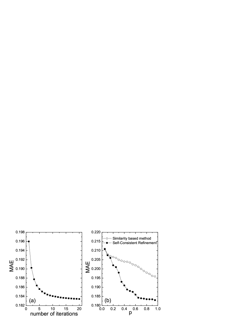
Figure 1: (a) Prediction error vs. iteration step, with $p=0.9$ fixed. (b) The comparison of algorithmic accuracy between the standard similarity-based method and the similarity-based SCR for different $p$.

Spectrum-based SCR.—We here present a spectrum-based algorithm, which relies on the Singular Value Decomposition (SVD) of the rating matrix. Analogously, we use the matrix with subtraction of average ratings, $R^{\prime}$, instead of $R$. The SVD of $R^{\prime}$ is defined as Zhang2004 :

$$R^{\prime}=U\cdot S\cdot V^{T},$$ (12)

where $U$ is an $N\times N$ unitary matrix formed by the eigenvectors of $R^{\prime}R^{\prime T}$, $S$ is an $N\times M$ singular value matrix with nonnegative numbers in decreasing order on the diagonal and zeros off the diagonal, and $V^{T}$ is an $M\times M$ unitary matrix formed by the eigenvectors of $R^{\prime T}R^{\prime}$. The number of positive diagonal elements in $S$ equals $\texttt{rank}(R^{\prime})$.

We keep only the $k$ largest diagonal elements (also the $k$ largest singular values) to obtain a reduced $k\times k$ matrix $S_{k}$, and then, reduce the matrices $U$ and $V$ accordingly. That is to say, only the $k$ column vectors of $U$ and $k$ row vectors of $V^{T}$ corresponding to the $k$ largest singular values are kept. The reconstructed matrix reads:

$$R^{\prime}_{k}=U_{k}\cdot S_{k}\cdot V^{T}_{k},$$ (13)

where $U_{k}$, $S_{k}$ and $V^{T}_{k}$ have dimensions $N\times k$, $k\times k$ and $k\times M$, respectively. Note that, Eq. (13) is no longer the exact decomposition of the original matrix $R^{\prime}$ (i.e., $R^{\prime}_{k}\neq R^{\prime}$), but the closest rank-$k$ matrix to $R$ Horn1985 . In other words, $R^{\prime}_{k}$ minimizes the Frobenius norm $\|R^{\prime}-R^{\prime}_{k}\|$ norm over all rank-$k$ matrices. Previous studies found that Berry1995 the reduced dimensional approximation sometimes performs better than the original matrix in information retrieval since it filters out the small singular values that may be highly distorted by the noise.

Actually, each row of the $N\times k$ matrix $U_{k}\sqrt{S_{k}}$ represents the vector of the corresponding agent’s tastes, and each row of the $M\times k$ matrix $V_{k}\sqrt{S_{k}}$ characterizes the features of the corresponding item. Therefore, the prediction of the evaluation a user $i$ gives to an item $\alpha$ can be obtained by computing the inner product of the $i$-th row of $U_{k}\sqrt{S_{k}}$ and the $\alpha$-th row of $V_{k}\sqrt{S_{k}}$:

$$\tilde{R} = U_{k}\sqrt{S_{k}}\cdot(V_{k}\sqrt{S_{k}})^{T}=U_{k}\sqrt{S_{k}}\cdot\sqrt{S_{k}}V_{k}^{T}$$ (14)

$$= U_{k}\cdot S_{k}\cdot V^{T}_{k}=R_{k}.$$

This derivation reproduces the Eq. (13), and illuminates the reason why using SVD to extract hidden information in user-item rating matrix. The entry $\tilde{R}_{i\alpha}$ is the predicted rating of user $i$ on item $\alpha$.

An underlying assumption in the $k$-truncated SVD method is the existence of $k$ principle attributes in both the user’s tastes and the item’s features. For example, a movie’s attributes may include the director, hero, heroine, gut, music, etc., and a user has his personal tastes on each attribute. If a movie is well fit his tastes, he will give a high rating, otherwise a low rating. Denote the states of a user $i$ and an item $\alpha$ as:

$$\langle u_{i}|=(u^{1}_{i},u^{2}_{i},\cdots,u^{k}_{i});\langle v_{\alpha}|=(v^{1}_{\alpha},v^{2}_{\alpha},\cdots,v^{k}_{\alpha}),$$ (15)

then we can estimate the evaluation of $i$ on $\alpha$ as the matching extent between their tastes and features:

$$\tilde{R}_{i\alpha}=\langle u_{i}|v_{\alpha}\rangle.$$ (16)

Therefore, we want to find a matrix $\tilde{R}$ that can be decomposed to $N$ $k$-dimensional taste vectors and $M$ $k$-dimensional feature vectors so that the corresponding entries are exactly the same as the known ratings and consequently, the other entries are the predicted ratings.

However, the $k$-truncated SVD matrix is not self-consistent for the elements corresponding to the known ratings in $R^{\prime}_{k}$ are not exactly the same as those in $R^{\prime}$. A self-consistent prediction matrix can be obtained via an iterative $k$-truncated SVD process by resetting those elements back to the known values at each step. Referring to Eq. (3), the Spectrum-based SCR treats the known ratings as the boundary conditions, and use $k$-truncated SVD as the matrix operator $\mathfrak{D}$. The iteration will converge to a stable matrix $\tilde{R}$, namely the predicted matrix.

Figure 2: (a) Prediction error vs. iteration step, with $p=0.9$ fixed. (b) The comparison of algorithmic accuracy between the standard spectrum-based method and the spectrum-based SCR for different $p$.

Numerical results.—To test the algorithmic accuracy, we use a benchmark data set, namely MovieLensdata . The data consists of $N=3020$ users, $M=1809$ movies, and $2.24\times 10^{5}$ discrete ratings 1-5. All the ratings are sorted according to their time stamps. We set a fraction $p$ of earlier ratings as the training set, and the remain ratings (with later time stamps) as the testing set.

As shown in Figs. 1 and 2, both the similarity-based and spectrum-based SCRs converge very fast, and sharply improve the algorithmic accuracy of the standard methods. In spectrum-based methods, the parameter $k$ is not observable in the real system, thus we treat it as a tunable parameter. The results displayed in Fig. 2 correspond to the optimal $k$ that minimizes the prediction error. For different $p$, the optimal $k$ is different. Denoting the data density as $\rho=E/NM$, where $E$ is the number of ratings in the training set. The spectrum-based SCR will converge only if $k$ is smaller than a threshold

$$k_{c}=\frac{N+M-2}{2}-\sqrt{\left(\frac{N+M-2}{2}\right)^{2}-NM\rho}\approx\frac{NM\rho}{N+M-2}.$$ (17)

So that the searching horizon of optimal $k$ can be reduced to the natural numbers not larger than $k_{c}$. The mathematical derivation and numerical results about this threshold behavior, as well as the sensitivity of algorithmic performance to $k$ will be discussed elsewhere.

Conclusions.—In this Letter, we proposed a algorithmic framework for recommender systems, namely self-consistent refinement. This general framework is implemented by embedding two representative recommendation algorithms: similarity-based and spectrum-based methods. Numerical simulations on a benchmark data set demonstrate the significant improvement of algorithmic accuracy compared with the standard algorithms. Actually, the spectrum-based SCR has higher accuracy than the similarity-based one, but it requires an optimizing process on the selection of the parameter $k$, thus takes longer computational time.

Besides the similarity-based and spectrum-based methods, very recently, some new kinds of recommendation algorithms that mimic certain physics dynamics, such as heat conduction Zhang2007a and mass diffusion Zhang2007b , are suggested to be the promising candidates in the next generation of recommender systems for they provide better algorithmic accuracy while have lower computational complexity. It is worthwhile to emphasize that those two algorithms Zhang2007a ; Zhang2007b also belong to the framework of SCR - they are just two specific realizations of SCR if considering the matrix operator $\mathfrak{D}$ as the conduction of heat or the exchange of mass during one step. In fact, the SCR framework is of great generality, and any algorithm that can be expressed in the form of Eq. (2) has the opportunity being improved via iterative SCR. Furthermore, the present method can be applied in not only the recommender systems, but also many other subjects, such as data clustering, miss data mining, detection of community structure, pattern recognition, predicting of protein structure, and so on.

This work is partially supported by SBF (Switzerland) for financial support through project C05.0148 (Physics of Risk), and the Swiss National Science Foundation (205120-113842). T.Z. acknowledges NNSFC under Grant No. 10635040 and 60744003, as well as the 973 Project 2006CB705500.

References

- (1) G. Linden et al., IEEE Internet Computing 7, 76 (2003).
- (2) D. Billsus et al., Commun. ACM 45, 34 (2002).
- (3) J. L. Herlocker et al., ACM Trans. Inform. Syst. 22, 5 (2004).
- (4) G. Adomavicius et al., IEEE Trans. Knowl. Data Eng. 17, 734 (2005).
- (5) A. Ansari et al., J. Mark. Res. 37, 363 (2000).
- (6) Y. P. Ying et al., J. Mark. Res. 43, 355 (2006).
- (7) R. Kumar et al., J. Comput. Syst. Sci. 63, 42 (2001).
- (8) J. O’Donovan et al., Proc. 10th Int’l Conf. Intell. User Interfaces (2005).
- (9) S. Maslov et al., Phys. Rev. Lett. 87, 248701 (2001).
- (10) P. Laureti et al., EPL 75, 1006 (2006).
- (11) Y.-C. Zhang et al., Phys. Rev. Lett. 99, 154301 (2007).
- (12) Y.-C. Zhang et al., EPL 80, 68003 (2007).
- (13) T. Zhou et al., Phys. Rev. E 76, 046115 (2007).
- (14) T. Zhou et al., EPL 81, 58004 (2008).
- (15) C.-K. Yu et al., Physica A 371, 732 (2006).
- (16) M. Blattner et al., Physica A 373, 753 (2007).
- (17) M. J. Pazzani et al., Lect. Notes Comput. Sci. 4321, 325 (2007).
- (18) J. A. Konstan et al., Commun. ACM 40, 77 (1997).
- (19) B. Sarwar et al., Proc. 10th Int’l WWW Conf. (2001).
- (20) D. Billsus et al., Proc. Int’l Conf. Machine Learning (1998).
- (21) B. Sarwar et al., Proc. ACM WebKDD Workshop (2000).
- (22) P. Resnick et al., Proc. Comput. Supported Cooperative Work Conf. (1994).
- (23) J. S. Breese et al., Proc. 14th Conf. Uncertainty in Artificial Intelligence (1998).
- (24) G. H. Golub et al., Matrix Computation (Baltimore, Johns Hopkins University Press, 1996).
- (25) X. Zhang, Matrix Analysis and Applications (Beijing, Tsinghua University Press & Springer, 2004).
- (26) R. A. Horn et al., Matrix analysis (Cambridge University Press, 1985).
- (27) The Fribenius norm (also called Euclidean norm, Schui norm or Hilbert-Schmidt norm) of a matrix , is defined as .
- (28) M. W. Berry et al., SIAM Rev. 37, 573 (1995).
- (29) The MovieLens data can be download from the website of GroupLens Research (http://www.grouplens.org).