NEW PHYSICS AT THE LHC: A LES HOUCHES REPORT
Physics at TeV Colliders 2007 – New Physics Working Group

Abstract

We present a collection of signatures for physics beyond the standard model that need to be explored at the LHC. The signatures are organized according to the experimental objects that appear in the final state, and in particular the number of high $p_{T}$ leptons. Our report, which includes brief experimental and theoretical reviews as well as original results, summarizes the activities of the “New Physics” working group for the “Physics at TeV Colliders” workshop (Les Houches, France, 11–29 June, 2007).

Abstract

Minimal Universal Extra Dimensions (MUED) models predict the presence of massive Kaluza-Klein particles decaying to final states containing Standard Model leptons and jets. The multi-lepton final states provide the cleanest signature. The ability of the CMS detector to find MUED final state signals with four electrons, four muons or two electrons and two muons was studied. The prospect of distinguishing between MUED and the Minimal Supersymmetric Standard Model (MSSM) is then discussed using simulations from the event generator Herwig++.

Abstract

If technicolor is responsible for electroweak symmetry breaking, there are strong phenomenological arguments that its energy scale is at most a few hundred GeV and that the lightest technihadrons are within reach of the ATLAS and CMS experiments at the LHC. Furthermore, the spin-one technihadrons $\rho_{T}$, $\omega_{T}$ and $a_{T}$ are expected to be very narrow, with striking experimental signatures involving decays to pairs of electroweak gauge bosons ($\gamma$, $W$, $Z$) or an electroweak boson plus a spin-zero $\pi_{T}$. Preliminary studies of signals and backgrounds for such modes are presented. With luminosities of a few to a few tens of femtobarns, almost all the spin-one states may be discovered up to masses of about 600 GeV. With higher luminosities, one can observe decay angular distributions and technipions that establish the underlying technicolor origin of the signals. Preliminary ATLAS studies show that, with $50$–$100\,{\rm fb}^{-1}$ and assuming $M_{a_{T}}\simeq 1.1M_{\rho_{T}}$, both processes $\rho_{T}^{\pm},\,a_{T}^{\pm}\rightarrow Z^{0}W^{\pm}$ (with $M_{\rho_{T}}\simeq 500\,{\rm GeV}$) may be seen in the $\ell^{+}\ell^{-}\ell^{\pm}\nu_{\ell}$ final state and $\rho_{T}^{\pm},\,a_{T}^{\pm}\rightarrow Z^{0}\pi_{T}^{\pm}$ (up to $M_{\rho_{T}}\simeq 400\,{\rm GeV}$) in $\ell^{+}\ell^{-}b\,{\rm jet}$, where $\ell=e,\,\mu$.

Abstract

Assuming composite spin-1 states to be the most relevant particles produced by EW scale strong interactions, we model them with a simple parametrization inspired by extra dimensions. Our flexible framework accommodates deviations from a QCD-like spectrum and interactions, as required by precision electroweak measurements.

Abstract

We propose a model-independent framework applicable to searches for new physics in the dilepton channel at the Large Hadron Collider. The feasibility of this framework has been demonstrated by the DØ searches for large extra dimensions. The proposed framework has a potential to distinguish between various types of models and determine most favorable parameters within a particular model, or set limits on their values.

Abstract

The rapidity distribution of a $Z^{\prime}$ produced at the LHC encodes information about the relative sizes of the couplings to up quarks and down quarks which is different from the inclusive cross section. Thus, by measuring the $Z^{\prime}$ production rate at different rapidities, we can help pin down the coupling to up quarks independently from the coupling to down quarks.

Abstract

A natural, non-supersymmetric solution to the hierarchy problem generically requires fermionic partners of the top quark with masses not much heavier than $500\,\text{GeV}$. We study the pair production and detection at the LHC of the top partners with electric charge $Q_{e}=5/3$ ($T_{5/3}$) and $Q_{e}=-1/3$ ($B$), that are predicted in models where the Higgs is a pseudo-Goldstone boson. Both kinds of new fermions decay to $Wt$, leading to a $t\bar{t}WW$ final state. We focus on the golden channel with two same-sign leptons, that offers the best chances of discovery in the very early phase of LHC and permits a full mass reconstruction of the $T_{5/3}$. Samples are processed with the CMS Fast Simulation.

Abstract

We review top quark pair production as a way to probe new physics at the LHC. Our scheme requires identifying integer-spin resonances from $t\bar{t}$ semileptonic decays in order to favor/disfavor new models of electroweak physics. The spin of each resonance can be determined by the angular distribution of top quarks in their c.m. frame. In addition, forward-backward asymmetry and CP-odd variables can be constructed to further distinguish the new physics. We parametrize the new resonances with a few generic parameters and show high invariant mass top pair production may provide a framework to distinguish models of new physics beyond the Standard Model.

Abstract

We consider the Randall–Sundrum model with fields propagating in the bulk and study the production of the strongly and weakly interacting gauge boson Kaluza–Klein excitations at the LHC. These states have masses of order of a few TeV and can dominantly decay into top quark pairs. We perform a Monte Carlo study of the production process $pp\to t\bar{t}$ in which the Kaluza–Klein excitations are exchanged and find that the latter can lead to a significant excess of events with respect to the Standard Model prediction.

Abstract

The twin Higgs mechanism has recently been proposed to solve the little hierarchy problem. We study the LHC collider phenomenology of the left-right twin Higgs model. We focus on the cascade decay of the heavy top partner, with a signature of multiple $b$ jets $+$ lepton $+$ missing energy. We also present the results for the decays of heavy gauge bosons: $W_{H}\rightarrow t\bar{b}$, $W_{H}\rightarrow\phi^{\pm}\phi^{0}$ and $Z_{H}\rightarrow e^{+}e^{-}$.

Abstract

In this report we intend first to review the main models where strong dynamics are responsible for EWSB. An overview of tests of new models through the production of new resonant states at the LHC is presented. We illustrate how different models can be related by looking at two general models with resonances.

Abstract

We review the motivation and main features of vector-like quarks with special emphasis on the techniques used in the calculation of the features relevant for their collider implications.

Abstract

At the LHC, the top-partner ($T_{-}$) and its antiparticle is produced in pairs in the Littlest Higgs model with T-parity. Each top-partner decays into top quark ($t$) and the lightest $T$-odd gauge partner $A_{H}$, and $t$ decays into three jets. We demonstrate the reconstruction of $t$ decaying hadronically, and measure the top-partner mass from the $m_{T2}$ distribution. We also discuss the dependency on four jet reconstruction algorithms (simple cone, kt, Cambridge, SISCone).

Abstract

We discuss prospects to search for a new massless neutral gauge boson, the paraphoton, in $e^{+}e^{-}$ collisions at center-of-mass energies of 0.5 and 1 TeV. The paraphoton naturally appearing in models with abelian kinetic mixing has interactions with the Standard Model fermion fields being proportional to the fermion mass and growing with energy. At the ILC, potentially the best process to search for the paraphoton is its radiation off top quarks. The event topology of interest is a pair of acoplanar top quark decaying to jets and missing energy. Applying a multivariate method for signal selection expected limits for the top-paraphoton coupling are derived. Arguments in favor of the missing energy as the paraphoton with spin 1 are shortly discussed.

Abstract

At the LHC objects with masses at the electroweak scale will for the first time be produced with very large transverse momenta. In many cases, these objects decay hadronically, producing a set of collimated jets. This interesting new experimental phenomenology requires the development and tuning of new tools, since the usual reconstruction methods would simply reconstruct a single jet. This study describes the application of the YSplitter algorithm in conjunction with the jet mass to identify high transverse momentum top quarks decaying hadronically.

Abstract

We propose to combine and slightly extend two existing “Les Houches Accords” to provide a simple generic interface between beyond-the-standard-model parton-level and event-level generators. All relevant information — particle content, quantum numbers of new states, masses, cross sections, parton-level events, etc — is collected in one single file, which adheres to the Les Houches Event File (LHEF) standard.

Part 1 Introduction

G. Brooijmans, A. Delgado, B.A. Dobrescu, C. Grojean and M. Narain

The exploration of the energy frontier will soon enter a dramatic new phase. With the startup of the LHC, planned for later this year, collisions at partonic center-of-mass energies above the TeV scale will for the first time be observed in large numbers.

The Standard Model currently provides an impressively accurate description of a wide range of experimental data. Nevertheless, the seven-fold increase in the center-of mass energy compared to the current highest-energy collider, the Tevatron, implies that the LHC will probe short distances where physics may be fundamentally different from the Standard Model. As a result, there is great potential for paradigm-changing discoveries, but at the same time the lack of reliable predictions for physics at the TeV scale makes it difficult to optimize the discovery potential of the LHC.

The TeV scale has been known for more than 30 years to be the energy of collisions required for revealing the origin of electroweak symmetry breaking. The computation of the amplitude for longitudinal $WW$ scattering [1] shows that perturbative unitarity is violated unless certain new particles exist at the TeV scale. More precisely, either a Higgs boson or some spin-1 particles that couple to $WW$ (as in the case of Technicolor or Higgsless models) are within the reach of the LHC, or else quantum field theory is no longer a good description of nature at that scale.

Given that ATLAS and CMS are multi-purpose detectors, it is commonly believed that they will provide such an in-depth exploration of the TeV scale that the nature of new physics will be revealed. Although this is likely to be true, one should recognize that the backgrounds will be large, and an effective search for the manifestations of new physics would require a large number of analyses dedicated to particular final states. Other than the unitarity of longitudinal $WW$ scattering, there are no clear-cut indications of what the ATLAS and CMS experiments might observe. Furthermore, recent theoretical developments have shown that the range of possibilities for physics at the TeV scale is very broad. Many well-motivated models predict various new particles which may be tested at the LHC. Hence, it would be useful to analyze as many of them as possible in order to ensure that the triggers are well-chosen and that the physics analyses have sufficient coverage.

The purpose of this report is to provide the LHC experimentalists with a collection of signatures for physics beyond the Standard Model organized according to the experimental objects that appear in the final state. The next four sections are focused on final states that include, in turn, three or more leptons, two leptons, a single lepton, and no leptons. Section 6 then describes an interface for event generators used in searches for physics beyond the Standard Model.

Whatever the nature of TeV scale physics is, the LHC will advance the understanding of the basic laws of physics. We hope that this report will help the effort of the particle physics community of pinning down the correct description of physics at the TeV scale.

blabla

Multi-Lepton Final States

Part 2 Four leptons + missing energy from one UED

M. Gigg and P. Ribeiro

1 DISCOVERY POTENTIAL FOR THE FOUR LEPTON FINAL STATE

1.1 Introduction

The Universal Extra Dimensions (UED) model [2] is an extension of the sub-millimeter extra dimensions model (ADD) [3, 4] in which all Standard Model (SM) fields, fermions as well as bosons, propagate in the bulk. In the minimal UED (MUED) scenario [5] only one Extra Dimension (ED) compactified on an orbifold is needed to create an infinite number of excitation modes of Kaluza-Klein (KK) particles with the same spin and couplings as the corresponding SM particles. The mass spectrum of the KK particles is defined by three free parameters: $\rm R^{-1}$, the size of the ED, given in terms of the compactification radius; $\Lambda$R, the number of excitation modes (KK levels) allowed in the effective theory; and $\rm m_{H}$, the SM Higgs boson mass. KK partners are indicated with the subscript related to the $n$-th mode of excitations (e.g. at the first level they are $\rm g_{1},Z_{1},u_{L1},e_{R1},\gamma_{1}$). A direct search for MUED in the multi-lepton channel at Tevatron energy of 1.8 TeV [6] set a lower bound on the size of ED of $\rm R^{-1}>280\leavevmode\nobreak\ \rm{GeV}$. Also, constraints from dark matter infer $600\leavevmode\nobreak\ <\rm{R^{-1}}<1050\leavevmode\nobreak\ \rm{GeV}$  [7].

In this section a summary report on the discovery potential of the CMS experiment [8] for MUED is presented. The complete analysis is described in [9]. The experimental signatures for production of first level KK states at hadron colliders are isolated leptons and/or jets radiated in the cascade decay process, in addition to the transverse missing energy carried away by the lightest KK particle (LKP). These characteristics were exploited to discriminate the signal from the background. The four lepton final state constitutes the cleanest channel. The KK mass spectrum, however, is highly degenerate since the masses of the KK particles with respect to the corresponding SM particles at tree level are $m_{n}^{2}={n}^{2}/R^{2}+m_{SM}^{2}$, where $n$ is the excitation mode. Furthermore, radiative corrections do not introduce an additional large splitting and typically, within the same excitation mode, there is a difference of about 100 GeV between the heaviest and the lightest KK particle. Therefore, the average values of the lepton momentum and the missing transverse energy are typically smaller than average values which characterise searches for supersymmetric events.

1.2 Signal and background processes

The MUED signal is produced in a $\rm{pp}$ collision as a pair of two KK strongly interacting particles, gluons ($\rm g_{1}$) or quarks ($\rm q_{1}$). Three significant subprocesses were considered:

$pp\rightarrow g_{1}g_{1},\leavevmode\nobreak\ \leavevmode\nobreak\ pp\rightarrow Q_{1}/q_{1}Q_{1}/q_{1},\leavevmode\nobreak\ \leavevmode\nobreak\ pp\rightarrow g_{1}Q_{1}/q_{1},$

Singlet and doublet KK quarks of the first generation were taken into account. Four points of the MUED parameter space have been chosen for the study: $\rm{m_{H}=120\,GeV}$, $\rm{\Lambda R=20}$ and $\rm{R^{-1}\in\{300,500,700,900\}\,GeV}$. The total cross section strongly depends on the compactification radius being equal to 2190, 165, 26 and 5.86 pb for $\rm{R^{-1}}=300,500,700$ and $900$ GeV respectively. The four lepton final state signature can provide a discrimination against the SM background and is considered as in the following:

$$g_{1}\rightarrow Q_{1}Q\,,\leavevmode\nobreak\ \leavevmode\nobreak\ Q_{1}\rightarrow Z_{1}Q\,,\leavevmode\nobreak\ \leavevmode\nobreak\ Z_{1}\rightarrow L_{1}\ell^{\pm},\leavevmode\nobreak\ \leavevmode\nobreak\ L_{1}\rightarrow LKP(\gamma_{1})\ell^{\mp}.$$ (1)

The KK gluon ($\rm g_{1}$) decays into a KK quark ($\rm q_{1}$) and a SM anti-quark; then, the $\rm q_{1}$ decays into the KK boson (Z₁) and a SM quark. Subsequently, Z₁ decays into a pair of leptons, one being a KK lepton ($\rm l_{1}\equiv$ singlet $\rm l_{R1}$ or, mainly, doublet $\rm l_{L1}$). Finally, $\rm l_{1}$ can decay only into the LKP photon ($\gamma_{1}$) and a SM lepton. Instead, if $\rm q_{1}$ is produced initially, then the decay cascade is shorter. The B.R. of the four lepton final state is about $\ 10^{-4}-10^{-3}$. Within a decay branch the pair of SM leptons ($\ell^{\pm}\ell^{\mp}$) has the same flavour and opposite sign. Three possible combinations of four leptons arise, namely 4$e$, 4$\mu$ and 2$e$2$\mu$, studied in three separated channels. Signal events were generated with CompHEP with particle definitions and Feynman rules taken from [10] at the LO approximation. The background to MUED signals results from SM processes with four leptons in the final state. The dominant sources are from the continuum production of $\rm{(Z^{*}/\gamma^{*})(Z^{*}/\gamma^{*})}$ and real $\rm{ZZ}$ production, from processes involving pair production of heavy quark flavours such as $\rm{t\bar{t}}$ and $\rm{b\bar{b}b\bar{b}}$, and the associated production of $\rm{Zb\bar{b}}$. Background events were generated with PYTHIA and ALPGEN. Signal and background events were processed with full detector simulation using official CMS software (OSCAR version 3.6.5). Underlying events from minimum bias interactions were superimposed to generated events, assuming an average number of 5 inelastic collisions, including diffractive interactions, at each beam crossing, simulating the effect of pile-up at $\rm{\mathcal{L}}=2\cdot 10^{33}\rm{cm^{-2}s^{-1}}$ (LHC low luminosity scenario). The reconstruction of physics objects was based on the dedicated CMS software ORCA (version 8.7.3/4).

1.3 Event Selection

First, Level 1 (L1) and High Level trigger (HLT) requirements for $\rm{\mathcal{L}}=2\cdot 10^{33}\rm{cm^{-2}s^{-1}}$ are applied to the simulated events. We then require the presence of at least two pairs of OSSF leptons. The leptons should be isolated (4 iso) and are required to be within the following kinematical boundaries ($\varepsilon_{2}$):

$\bullet$	electrons with $p_{T}$ $>$7.0 GeV and $|\eta|<$ 2.5,
$\bullet$	muons     with $p_{T}$ $>$5.0 GeV and $|\eta|<$ 2.4.

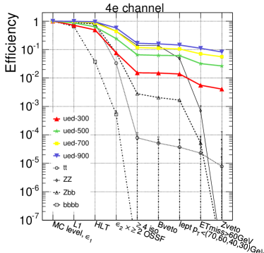
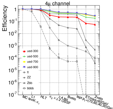
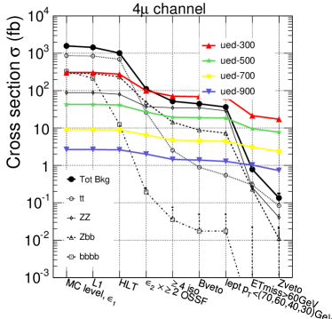
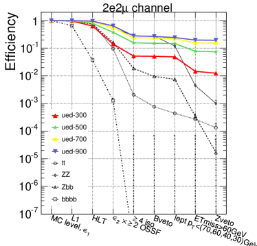
Because a substantial fraction of the background leptons results from b-quark leptonic decays, we reject events where one or more b-jets are identified (Bveto). Due to the soft KK mass spectrum, leptons from the MUED cascade (eq. 1) have on average lower transverse momentum than some of the background channels, like for example the background from top quark decays. For this reason we apply upper bound cuts on the lepton transverse momentum (lept $\rm{p_{T}}$) of 70, 60, 40, 30 GeV for the $1^{st},2^{nd},3^{rd},4^{th}$ lepton sorted in $p_{T}$, respectively. A missing transverse energy cut of ${\rm E_{T}/\hskip 5.69046pt}>60$ GeV proves to be important especially for high $\rm{R^{-1}}$ values where the ${\rm E_{T}/\hskip 5.69046pt}$ is higher due to the massive LKPs, as the background is significantly rejected with respect to a small reduction of signal events. Finally, we apply a selection on the invariant mass of the lepton pairs, according to which an event is rejected if it has one or more OSSF lepton pair with $\rm M_{inv}<5$ GeV or $\rm M_{inv}>80$ GeV, aimed at rejecting the $\rm{ZZ}$ background. The selection cuts were chosen so that the signal efficiency is maximum for ($\rm{R^{-1}=900}$ GeV), where the signal cross section is lowest.

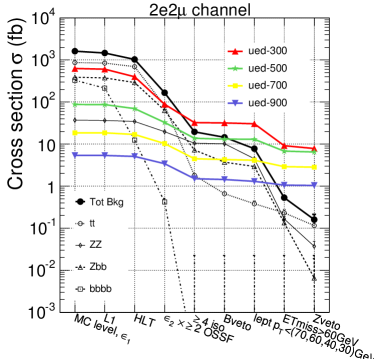
The summary of all selection cuts is presented in figure 1 in two ways: as an efficiency of each cut after the previous one (left), and as a cross section after each cut (right). After all selection cuts, a S/B greater than five is achieved for all studied points of the parameter space.

Figure 1: Cumulative efficiency and cross section after each selection cut for the MUED signal ($\mathrm{R^{-1}}\in\{300,500,700,900\}$ GeV, $\rm m_{H}=120$ GeV, $\Lambda\mathrm{R}=20$) and the background for all channels. Only the upper statistical uncertainties are shown.

1.4 Results

The CMS discovery potential of MUED in the four lepton channel, defined as the integrated luminosity needed to measure a signal with a significance ($\rm S_{cP}$) of five standard deviations is shown in figure 2. The significance estimator S_cP gives the probability to observe a number of events equal or greater than $\rm N_{obs}=N_{Signal}+N_{Bkg}$, assuming a background-only hypothesis, converted to the equivalent number of standard deviations of a Gaussian distribution. The dashed (solid) lines show results including (not including) systematical uncertainties. The systematic uncertainties include a 20% uncertainty on the background cross section, the effect of jet energy scale on the missing energy distribution (3-10%, $p_{T}$ dependent) and a 5% uncertainty in the b-tagging algorithm efficiency. For the three four-lepton channels ( 4$e$, 4$\mu$ and 2$e$2$\mu$) and for the integrated luminosity of 30 $fb^{-1}$ , the signal significance is above the background by a few standard deviations and therefore the MUED signal could be detected at the CMS experiment during the first few years of data taking. In the 4$\mu$ and the 2$e$2$\mu$ channels alone, a significance of five standard deviations for $R^{-1}=500$ GeV could be reached with less than one $fb^{-1}$ of data.

Figure 2: The discovery potential of MUED signals ($\mathrm{R^{-1}}\in\{300,500,700,900\}$ GeV, $\rm m_{H}=120$ GeV, $\Lambda\mathrm{R}=20$) in the four-lepton channels is defined as the integrated luminosity needed to measure a signal with a significance ($\rm S_{cP}$) of five standard deviations. The dashed (solid) lines show results including (not including) systematical uncertainties. The uncertainties due to the limited understanding of the detector performance and characteristic of the early phase of the LHC data taking are not considered and may limit the sensitivity below one $fb^{-1}$(horizontal ’First data uncertainty’ line).

2 MODEL DISCRIMINATION

The four lepton channel described above can also produced in supersymmetry (SUSY). The focus of this section will be in comparison of different signatures from SUSY and UED using the monte carlo event generator Herwig++.

As of version 2.1 of Herwig++ [11] BSM physics was included for the first time with both the minimal supersymmetric standard model (MSSM) and minimal universal extra dimensions models implemented including spin correlations in production and decay [12]. This allows the comparative study of both models within the same general purpose event generator. To compare the two models in the most sensible manner the mass spectra should be the same. The simplest way to achieve this is to chose a scale for the MUED model and then adjust the parameters in the MSSM so that the relevant masses are matched. Two scales were chosen for this work, $\mathrm{R^{-1}=500\,GeV}$ and $\mathrm{R^{-1}=900\,GeV}$, both with $\Lambda R=20$ which produced the mass spectra shown in tables 1 and 2. The MSSM spectrum file and decay tables were produced using SDECAY version 1.3 [13].

$g_{1}$	$q_{L1}$	$u_{R1}$	$d_{R1}$	$l_{L1}$	$\gamma_{1}$
626.31	588.27	576.31	574.90	514.78	500.98

Table 1: The UED mass spectrum for $\mathrm{R^{-1}=500\,GeV}$ and $\Lambda R=20$. The SUSY counterparts are matched to this. All values are in GeV.

$g_{1}$	$q_{L1}$	$u_{R1}$	$d_{R1}$	$l_{L1}$	$\gamma_{1}$
1114.25	1050.50	1028.84	1025.28	926.79	900.00

Table 2: The UED mass spectrum for $\mathrm{R^{-1}=900\,GeV}$ and $\Lambda R=20$. The SUSY counterparts are matched to this. All values are in GeV.

The previous section tells us that the four lepton channel could give a sizeable signal compared to the standard model background. Plotting the invariant mass distribution of the di-muon pairs in a four muon final state event for MUED and SUSY gives the results shown in figure 3. It is apparent that larger values of the masses within the spectrum make it more difficult to distinguish between the two models. Moreover, in the $\mathrm{R^{-1}=500\,GeV}$ case the shapes of the distributions are similar it is just the overall number of events in the SUSY case that is larger due to the size of the relative branching ratios. Given the possibility that the distributions could be so similar it will be necessary to make use of other combinations of invariant mass plots. The most logical is the invariant mass of a quark plus one of the lepton or antileptons. Since it is possible to distinguish between leptons and antileptons in a detector one can make separate distributions for the jet plus lepton and the jet + antilepton cases. Since these now take into account the helicity of the quark these distributions will be more sensitive to spin effects.

Figure 3: The invariant mass of the di-muon pair coming from each chain in a four muon event for (a) $\mathrm{R^{-1}=500\,GeV}$ and (b) $\mathrm{R^{-1}=900\,GeV}$. Solid: UED, dot-dash: SUSY.

Figure 4 shows the invariant mass of a jet plus a lepton while figure 5 shows the distribution for a jet plus an antilepton for the two scales under consideration. Again there is a greater difference at a lower value of the compactification radius where it would seem that the shapes of the distributions differ more at higher invariant mass values. The main reason, however, for the similarity in the distributions under study is that they have combined effects from opposite sets of spin correlations. This result can be attributed to firstly the lack of distinction between quark and antiquark in the jet/lepton distributions which means that two sets of data with opposite spin correlations appear on the same plot thereby cancelling the effect out. Also the run was set up so that both left and right-handed partners to the quarks were produced in the initial hard collision and when these decay they will have, again, opposite correlations. It is these kinds of effect that will cause the most trouble in trying to distinguish between the two models.

Figure 4: The invariant mass of a quark or an antiquark with a lepton for (a) $\mathrm{R^{-1}=500\,GeV}$ and (b) $\mathrm{R^{-1}=900\,GeV}$. Solid: UED, dot-dash: SUSY.

Figure 5: The invariant mass of a quark or an antiquark with an antilepton for (a) $\mathrm{R^{-1}=500\,GeV}$ and (b) $\mathrm{R^{-1}=900\,GeV}$. Solid: UED, dot-dash: SUSY.

A useful quantity in trying to achieve this at the LHC will be the asymmetry, defined as

$$A^{\pm}=\left(\frac{dP}{dm_{jl^{+}}}-\frac{dP}{dm_{jl^{-}}}\right)/\left(\frac{dP}{dm_{jl^{+}}}+\frac{dP}{dm_{jl^{-}}}\right),$$ (2)

where $dP/dm_{jl^{+}}$ and $dP/dm_{jl^{-}}$ are the antilepton and lepton distributions respectively. Its usefulness stems from the fact that the LHC is a proton-proton collider and will produce an excess of quarks over antiquarks. The result will be a slight favour in one helicity mode over the other meaning the asymmetry should be the most sensitive to the underlying physics model. The distributions from Herwig++ are shown in figure 6.

Figure 6: The asymmetry, as defined in equation 2, for (a) $\mathrm{R^{-1}=500\,GeV}$ and (b) $\mathrm{R^{-1}=900\,GeV}$. Solid: UED, dot-dash: SUSY.

3 CONCLUSIONS

The CMS experiment will be able to detect evidence of MUED model in the four lepton final state up to $\rm{R^{-1}=900}$ GeV with an integrated luminosity of 30 $fb^{-1}$. For the purpose of discrimination between the MUED and SUSY scenarios it is apparent that the analysis of the four lepton signature alone is insufficient. The best hope is using asymmetry distribution as this is most sensitive to the spin differences in the underlying physics model.

ACKNOWLEDGEMENTS

The work of M. Gigg was supported by the Science and Technology Facilities Council and in part by the European Union Marie Curie Research Training Network MCnet under contract MRTN-CT-2006-035606. The work of P. Ribeiro was supported by Fundacao para a Ciencia e Tecnologia under grant SFRH/BD/16103/2004.

Part 3 LHC Events with Three or More Leptons Can Reveal Fermiophobic $W^{\prime}$ Bosons

R.S. Chivukula and E.H. Simmons

1 INTRODUCTION

Events with three or more leptons plus either jets or missing energy can lead to the discovery of fermiophobic $W^{\prime}$ bosons associated with the origin of electroweak symmetry breaking. One possibility is the process $pp\to(W^{\ast})\to W^{\prime(\ast)}Z\to WZZ\to\,jj\ell^{+}\ell^{-}\ell^{+}\ell^{-}$ where the $W$ is assumed to decay hadronically and $\ell$ can be an electron or muon. Another is the process $pp\to WZjj$ where the $W$ and $Z$ re-scatter through the $W^{\prime}$ resonance; the final state of interest here includes three leptons, two jets, and missing energy. This section describes a general class of “Higgsless” models that include fermiophobic $W^{\prime}$ bosons, specify the particular model used in our phenomenological studies, and then describe the calculations and results for each multi-lepton channel in turn.

The $pp\to WZjj$ signal is the classic $WW$-scattering process studied for a strongly interacting symmetry breaking sector, with the $W^{\prime}$ playing an analogous role to the technirho boson. In the three-site higgsless model considered below it is possible to calculate this process in a fully gauge-invariant manner, rather than using the traditional method that involves separately calculating the signal (by using a model of $\pi\pi$ scattering in conjunction with the effective $W$ approximation) and background (usually done by considering the standard model with a light Higgs boson).

2 HIGGSLESS MODELS IN GENERAL

Higgsless models [15] provide electroweak symmetry breaking, including unitarization of the scattering of longitudinal $W$ and $Z$ bosons, without employing a scalar Higgs boson. The most extensively studied models [16, 17] are based on a five-dimensional $SU(2)\times SU(2)\times U(1)$ gauge theory in a slice of Anti-deSitter space, and electroweak symmetry breaking is encoded in the boundary conditions of the gauge fields. Using the AdS/CFT correspondence [18], these theories may be viewed as “dual” descriptions of walking technicolor theories [19, 20, 21, 22, 23, 24]. In addition to a massless photon and near-standard $W$ and $Z$ bosons, the spectrum includes an infinite tower of additional massive vector bosons (the higher Kaluza-Klein or $KK$ excitations), whose exchange is responsible for unitarizing longitudinal $W$ and $Z$ boson scattering [25]. To provide the necessary unitarization, the masses of the lightest $KK$ bosons must be less than about 1 TeV. Using deconstruction, it has been shown [26] that a Higgsless model whose fermions are localized (i.e., derive their electroweak properties from a single site on the deconstructed lattice) cannot simultaneously satisfy unitarity bounds and precision electroweak constraints.

The size of corrections to electroweak processes in Higgsless models may be reduced by considering delocalized fermions [27, 28, 29], i.e., considering the effect of the distribution of the wavefunctions of ordinary fermions in the fifth dimension (corresponding, in the deconstruction language, to allowing the fermions to derive their electroweak properties from several sites on the lattice). Higgsless models with delocalized fermions provide an example of a viable effective theory of a strongly interacting symmetry breaking sector consistent with precision electroweak tests.

It has been shown [30] that, in an arbitrary Higgsless model, if the probability distribution of the delocalized fermions is related to the $W$ wavefunction (a condition called “ideal” delocalization), then deviations in precision electroweak parameters are minimized. Ideal delocalization results in the $W^{\prime}$ resonances being fermiophobic. Phenomenological limits on delocalized Higgsless models may be derived [31] from limits on the deviation of the triple-gauge boson ($WWZ$) vertices from their standard model value; current constraints allow for the lightest $KK$ resonances to have masses as low as 400 GeV.

3 THREE-SITE MODEM IN PARTICULAR

Many issues of interest, such as ideal fermion delocalization and the generation of fermion masses (including the top quark mass) can be illustrated in a Higgsless model deconstructed to just three sites [32]. The electroweak sector of the three-site Higgsless model incorporates an $SU(2)_{0}\times SU(2)_{1}\times U(1)_{2}$ gauge group, and $2$ nonlinear $(SU(2)\times SU(2))/SU(2)$ sigma models responsible for breaking this symmetry down to $U(1)_{em}$. The extended electroweak gauge sector of the three-site model is that of the Breaking Electroweak Symmetry Strongly (BESS) model [33]. The mass-eigenstate vector bosons are admixtures of the seven gauge-bosons in $SU(2)^{2}\times U(1)$, with one massless photon, three corresponding to the standard model $W^{\pm}$ and $Z$, and three nearly-degenerate $W^{\prime\pm}$ and $Z^{\prime}$. For the reasons described above, the masses of the $W^{\prime\pm}$ and $Z^{\prime}$ in the three-site model (and indeed for the lightest bosons in any Higgsless model with ideal fermion delocalization) must be between roughly 400 GeV and 1 TeV.

The left-handed fermions are doublets coupling to the two $SU(2)$ groups, which may be correspondingly labeled $\psi_{L0}$ and $\psi_{L1}$. The right-handed fermions are a doublet coupling to $SU(2)_{1}$, $\psi_{R1}$, and two singlet fermions coupled to $U(1)_{2}$, denoted $u_{R2}$ and $d_{R2}$ in the case of quarks. The fermions $\psi_{L0}$, $\psi_{L1}$, and $\psi_{R1}$ have $U(1)$ charges typical of the left-handed doublets in the standard model, $+1/6$ for quarks and $-1/2$ for leptons. Similarly, the fermion $u_{R2}$ has $U(1)$ charges typical for the right-handed up-quarks (+2/3), and $d_{R2}$ has the $U(1)$ charge associated with the right-handed down-quarks ($-1/3$) or the leptons ($-1$). With these assignments, one may write the Yukawa couplings and fermion mass term

$${\cal L}_{f}=\varepsilon_{L}M\,\bar{\psi}_{L0}\Sigma_{1}\psi_{R1}+M\,\bar{\psi}_{R1}\psi_{L1}+M\,\bar{\psi}_{L1}\Sigma_{2}\begin{pmatrix}\varepsilon_{Ru}&\\ &\varepsilon_{Rd}\end{pmatrix}\begin{pmatrix}u_{R2}\\ d_{R2}\end{pmatrix}+h.c.$$ (1)

Here the Dirac mass $M$ is typically large (of order 2 or more TeV), $\varepsilon_{L}$ is flavor-universal and chosen to be of order $M_{W}/M_{W^{\prime}}$ to satisfy the constraint of ideal delocalization, and the $\varepsilon_{R}$ are proportional to the light-fermion masses (and are therefore small except in the case of the top-quark) [32]. These couplings yield a seesaw-like mass matrix, resulting in light standard-model-like fermion eigenstates, along with a set of degenerate vectorial doublets (one of each standard model weak-doublet).

The three-site model is sufficiently simple that it is possible to implement the model in CompHEP [34] or MADGRAPH [35], and – by including both fermion and gauge-boson couplings – to do so in a way that is fully gauge-invariant.

4 4 LEPTONS PLUS 2 JETS

LHC events with 4 charged leptons and 2 jets can reveal [36] the presence of a fermiophobic $W^{\prime}$ boson that is produced through $pp\to WZZ$ with the $Z$ bosons decaying leptonically and the $W$ decaying hadronically. The signal for the $W^{\prime}$ boson comes from associated production $pp\to(W^{\ast})\to W^{{}^{\prime}}Z$ followed by the decay $W^{\prime}\to WZ$. The backgrounds include the irreducible SM background $pp\to WZZ\to jj\ell^{+}\ell^{-}\ell^{+}\ell^{-}$; a related, but reducible, SM background $\,pp\to ZZZ\to jj\ell^{+}\ell^{-}\ell^{+}\ell^{-}\,$ in which the hadronically-decaying $Z$ is mis-identified as a $W$; and all other SM processes leading to the same final state $pp\to jj\ell^{+}\ell^{-}\ell^{+}\ell^{-}$ through different intermediate steps, including processes in which one or more of the jets is gluonic.

Ref. [36] has calculated the full signal and background in the context of the three-site higgsless model [32] using the cuts described here. One set of cuts is used to suppress the SM backgrounds:

$$M_{jj}\,=\,80\pm 15\,{\rm GeV},\leavevmode\nobreak\ \leavevmode\nobreak\ \leavevmode\nobreak\ \leavevmode\nobreak\ \leavevmode\nobreak\ \leavevmode\nobreak\ \Delta R(jj)\,<\,1.5\,,\leavevmode\nobreak\ \leavevmode\nobreak\ \leavevmode\nobreak\ \leavevmode\nobreak\ \leavevmode\nobreak\ \leavevmode\nobreak\ \sum_{Z}p_{T}^{\leavevmode\nobreak\ }(Z)+\sum_{j}p_{T}^{\leavevmode\nobreak\ }(j)\,=\,\pm 15\leavevmode\nobreak\ {\rm GeV}.$$ (2)

The first of these selects dijets arising from on-shell $W$ decay (leaving a margin for the experimental resolution [37]); the second reflects the dijet separation of the signal events; and the third exploits the conservation of transverse momentum in the signal events. In addition, a set of transverse momentum and rapidity cuts are imposed on the jets and charged leptons

$$p_{T\ell}^{\leavevmode\nobreak\ }>10\,{\rm GeV},\leavevmode\nobreak\ \leavevmode\nobreak\ \leavevmode\nobreak\ \leavevmode\nobreak\ \leavevmode\nobreak\ \leavevmode\nobreak\ |\eta_{\ell}^{\leavevmode\nobreak\ }|<2.5\,,\leavevmode\nobreak\ \leavevmode\nobreak\ \leavevmode\nobreak\ \leavevmode\nobreak\ \leavevmode\nobreak\ \leavevmode\nobreak\ p_{Tj}^{\leavevmode\nobreak\ }>15\,{\rm GeV},\leavevmode\nobreak\ \leavevmode\nobreak\ \leavevmode\nobreak\ \leavevmode\nobreak\ \leavevmode\nobreak\ \leavevmode\nobreak\ |\eta_{j}^{\leavevmode\nobreak\ }|<4.5\,.$$ (3)

for particle identification.

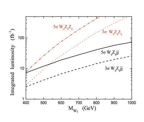
These cuts essentially eliminate the first two sources of background and reduce the third to a manageable size, with the signal peak standing out cleanly. Ref. [36] concludes that fermiophobic $W^{\prime}$ bosons will be visible in this channel at the LHC throughout their entire allowed mass range from $400-1200$ GeV. The integrated luminosity required for detecting the $W^{\prime}$ in this channel is shown here as a function of $W^{\prime}$ mass in Fig. 1.

5 3 LEPTONS PLUS MISSING ENERGY

LHC events with 3 charged leptons, missing energy, and forward jets can reveal the presence of a fermiophobic $W^{\prime}$ boson produced through the scattering process $pp\to WZqq^{\prime}$, where both vector bosons decay leptonically [38, 39, 40]. In this case, the signal arises from the $W^{\prime}$ contribution to the vector boson fusion subprocess $WZ\to WZ$.

An initial estimate of the $W^{\prime}$ signal and related backgrounds was presented in in ref. [41] for a 5d higgsless sum rule scenario. Ref. [36] has improved on this by performing the first tree-level calculation that includes both the signal and the full electroweak (EW) and QCD backgrounds for the $2\to 4$ scattering process  $pp\to WZjj^{\prime}$ in the context of a complete, gauge-invariant higgsless model (the three-site model [32]). A forward-jet tag is used to eliminate the reducible QCD background [38] from the annihilation process $qq\to WZ$. The irreducible QCD backgrounds $pp\to WZjj$ with $jj=qg,\,gg$ serving as forward jets are suppressed by the cuts

$$E_{j}>300\,{\rm GeV}\,,\leavevmode\nobreak\ \leavevmode\nobreak\ \leavevmode\nobreak\ \leavevmode\nobreak\ \leavevmode\nobreak\ \leavevmode\nobreak\ p_{Tj}>30\,{\rm GeV}\,,\leavevmode\nobreak\ \leavevmode\nobreak\ \leavevmode\nobreak\ \leavevmode\nobreak\ \leavevmode\nobreak\ \leavevmode\nobreak\ |\eta_{j}|<4.5\,,\leavevmode\nobreak\ \leavevmode\nobreak\ \leavevmode\nobreak\ \leavevmode\nobreak\ \leavevmode\nobreak\ \leavevmode\nobreak\ \left|\Delta\eta_{jj}\right|>4\,,$$ (4)

where $E_{j}$ and $p_{Tj}$ are transverse energy and momentum of each final-state jet, $\eta_{j}$ is the forward jet rapidity, and $\left|\Delta\eta_{jj}\right|$ is the difference between the rapidities of the two forward jets. The cut on $|\Delta\eta_{jj}^{\leavevmode\nobreak\ }|$ is especially good at suppressing the QCD backgrounds  $pp\to WZgg,\leavevmode\nobreak\ WZqg$  in the low $M_{WZ}$ region  [42]. The following lepton identification cuts are also employed

$$p_{T\ell}^{\leavevmode\nobreak\ }\,>\,10\,{\rm GeV}\,,\leavevmode\nobreak\ \leavevmode\nobreak\ \leavevmode\nobreak\ \leavevmode\nobreak\ \leavevmode\nobreak\ \leavevmode\nobreak\ \leavevmode\nobreak\ |\eta_{\ell}^{\leavevmode\nobreak\ }|\,<\,2.5\,.$$ (5)

While one must specify a reference value of the SM Higgs boson mass in computing the SM EW backgrounds, the authors of [36] found that varying the Higgs mass over the range $M_{H}=115\,{\rm GeV}-1\,$TeV had little effect.

Ultimately, ref. [36] reports both the signal and backgrounds for the transverse mass distribution of the vector boson pair, where $M_{T}^{2}(WZ)\equiv[\sqrt{M^{2}(\ell\ell\ell)+p_{T}^{2}(\ell\ell\ell)}+|p_{T}^{\rm miss}|]^{2}-|p_{T}(\ell\ell\ell)+p_{T}^{\;\rm miss}|^{2}$. Counting the signal and background events in the range $0.85M_{W^{\prime}}<M_{T}<1.05M_{W^{\prime}}$, yields the integrated LHC luminosities required for $3\sigma$ and $5\sigma$ detections of the $W^{\prime}$ boson in this channel, as shown here in Fig. 1.

Figure 1: Integrated luminosities required for $3\sigma$ and $5\sigma$ detection of $W^{\prime}$ signals as a function of $M_{W^{\prime}}$. The dotted and dashed-dotted curves are for the $WZZ$ channel, while the dashed and solid curves are for the $WZjj$ channel. From ref. [36].

6 CONCLUSIONS

Both the $pp\to W^{\prime}Z\to WZZ\to jj4\ell$ and $pp\to W^{\prime}jj\to WZjj\to\nu 3\ell\,jj$ channels are promising for revealing fermiophobic $W^{\prime}$ bosons, like those in Higgsless models, at the LHC [36]. The $WZZ$ channel has a distinct signal with a clean resonance peak. The $WZjj^{\prime}$ channel has a larger cross section when $M_{W^{\prime}}$ is heavy, but the measurement is complicated by the missing $E_{T}$ of the final-state neutrino. Hence, confirming the existence of both signals for the $W^{\prime}$ boson, as well as the absence of a Higgs-like signal in $pp\to ZZqq\to 4\ell\,qq$, will be strong evidence for Higgsless electroweak symmetry breaking  [36]. In particular, as shown here in Fig.  1, for $M_{W^{\prime}}=500\,(400)$ GeV, the $5\sigma$ discovery of $W^{\prime}$ requires an integrated luminosity of 26 (7.8) fb^-1 for $pp\to WZZ\to jj\,4\ell$, and 12 (7) fb^-1 for $pp\to WZjj\to\nu 3\ell\,jj$. These are within the reach of the first few years’ run at the LHC.

Part 4 Low-Scale Technicolor at the LHC

G. Azuelos, K. Black, T. Bose, J. Ferland, Y. Gershtein, K. Lane and A. Martin

1 INTRODUCTION

Technicolor (TC) is a proposed strong gauge interaction responsible for the dynamical breakdown of electroweak symmetry [43, 44]. Modern technicolor has a slowly-running (“walking”) gauge coupling [19, 22, 45, 46]. This feature allows extended technicolor (ETC) [47] to generate realistic masses for quarks, leptons and technipions ($\pi_{T}$) with the very large ETC boson masses ($10^{3}$–$10^{4}\,{\rm TeV}$) necessary to suppress flavor-changing neutral current interactions. (For reviews, see Refs. [48, 49].) The important phenomenological consequence of walking is that the technicolor scale is likely to be much lower and the spectrum of this low-scale technicolor (LSTC) much richer and more experimentally accessible [50, 51, 52] than originally thought [53]. The basic argument is this: (1) The walking TC gauge coupling requires either a large number $N_{D}$ of technifermion doublets so that $\Lambda_{TC}\simeq 250\,{\rm GeV}/\sqrt{\smash[b]{N_{D}}}\mathrel{\hbox to0.0pt{\raise 2.20013pt\hbox{$<$}\hss}{\lower 2.20013pt\hbox{$\sim$}}}100\,{\rm GeV}$, or two TC scales, one much lower than $250\,{\rm GeV}$. (2) Walking enhances $\pi_{T}$ masses much more than those of their vector partners, $\rho_{T}$ and $\omega_{T}$. This effect probably closes the all-$\pi_{T}$ decay channels of the lightest techni-vectors. In LSTC, then, we expect that the lightest $\rho_{T}$ and $\omega_{T}$ lie below about $0.5\,{\rm TeV}$ and that they decay to an electroweak boson ($\gamma$, $W$, $Z$) plus $\pi_{T}$; a pair of electroweak bosons; and $\bar{f}f$, especially $\ell^{+}\ell^{-}$. These channels have very distinctive signatures, made all the more so because $\rho_{T}$ and $\omega_{T}$ are very narrow, $\Gamma(\rho_{T})\simeq 1$–$5\,{\rm GeV}$ and $\Gamma(\omega_{T})\simeq 0.1$–$0.5\,{\rm GeV}$. Technipions are expected to decay via ETC interactions to the heaviest fermion-antifermion flavors allowed kinematically, providing the best chance of their being detected.

Many higher-mass states are reasonably expected in addition to $\rho_{T}$ and $\omega_{T}$. In Refs. [56, 57] it was argued that walking TC invalidates the standard QCD-based calculations of the precision-electroweak $S$-parameter [58, 59, 60, 61]. In particular, the spectral functions appearing in $S$ cannot be saturated by a single $\rho_{T}$ and its axial-vector partner $a_{T}$. Thus, walking TC produces something like a tower of vector and axial-vector isovector states above the lightest $\rho_{T}$ and $a_{T}$. All (or many) of them may contribute significantly to the $S$-parameter. Most important phenomenologically, in models with small $S$, the lightest $a_{T}$ and $\rho_{T}$ likely are nearly degenerate and have similar couplings to their respective weak vector and axial-vector currents; see, e.g., Refs. [62, 63, 64, 65, 66]. The $3\,\pi_{T}$-decay channels of the $a_{T}$ are closed, so these states are also very narrow, $\Gamma(a_{T})\mathrel{\hbox to0.0pt{\raise 2.20013pt\hbox{$<$}\hss}{\lower 2.20013pt\hbox{$\sim$}}}0.5\,{\rm GeV}$.

The $\rho_{T}$, $\omega_{T}$, $a_{T}$, and $\pi_{T}$ of low-scale technicolor that we consider are bound states of the lightest technifermion electroweak doublet, $(T_{U},T_{D})$. The phenomenology of these technihadrons is set forth in the “Technicolor Straw-Man Model” (TCSM) [67, 68, 66]. The TCSM’s most important assumptions are: (1) There are $N_{D}$ isodoublets of technifermions transforming according to the fundamental representation of the TC gauge group. The lightest doublet is an ordinary-color singlet. We use $N_{D}=9$ in calculations; then, the technipion decay constant $F_{T}\simeq 246\,{\rm GeV}/\sqrt{\smash[b]{N_{D}}}=82\,{\rm GeV}$. The technipion isotriplet composed of the lightest technifermions is a simple two-state admixture,

$$|\Pi_{T}^{\pm,0}\rangle=\sin\chi\,|W_{L}^{\pm,0}\rangle+\cos\chi\,|\pi_{T}^{\pm,0}\rangle\,,$$ (1)

where $W_{L}$ is a longitudinally-polarized weak boson and $\pi_{T}$ is a mass eigenstate, the lightest technipion referred to above, and $\sin\chi=F_{T}/246\,{\rm GeV}=1/\sqrt{\smash[b]{N_{D}}}$. This is why the lightest spin-one technihadrons are so narrow: all their decay amplitudes are suppressed by a power of $\sin\chi$ for each $W_{L}$ emitted and by a power of $e=g\sin\theta_{W}$ for each transversely-polarized $W_{\perp}$. In addition, decays to $\pi_{T}$ are phase-space limited. The technihadrons’ principal decay modes are listed in Table 1. (2) The lightest bound-state technihadrons may be treated in isolation, without significant mixing or other interference from higher-mass states. (3) Techni-isospin is a good symmetry. These assumptions allow the TCSM to be described by a relatively small number of parameters. The ones used for the present study are, we believe, fairly generic; they are listed below.

Process	$V_{V_{T}/a_{T}G\pi_{T}}$	$A_{V_{T}/a_{T}G\pi_{T}}$
$\omega_{T}\rightarrow\gamma\pi_{T}^{0}$	$\cos\chi$	0
$\thinspace\thinspace\thinspace\quad\rightarrow\gamma Z^{0}_{L}$	$\sin\chi$	0
$\thinspace\thinspace\thinspace\qquad\rightarrow W^{\pm}\pi_{T}^{\mp}$	$\cos\chi/(2\sin\theta_{W})$	0
$\,\,\,\;\;\qquad\rightarrow W^{\pm}W_{L}^{\mp}$	$\sin\chi/(2\sin\theta_{W})$	0
$\qquad\rightarrow Z^{0}\pi_{T}^{0}$	$\cos\chi\cot 2\theta_{W}$	0
$\,\qquad\rightarrow Z^{0}Z_{L}^{0}$	$\sin\chi\cot 2\theta_{W}$	0
$\rho_{T}^{0}\rightarrow W_{L}^{\pm}\pi_{T}^{\mp}$	$\sin\chi\cos\chi$	—
$\;\;\;\quad\rightarrow W_{L}^{+}W_{L}^{-}$	$\sin^{2}\chi$	—
$\;\rightarrow\gamma\pi_{T}^{0}$	$(Q_{U}+Q_{D})\cos\chi$	0
$\;\rightarrow\gamma Z_{L}^{0}$	$(Q_{U}+Q_{D})\sin\chi$	0
$\;\;\quad\rightarrow W^{\pm}\pi_{T}^{\mp}$	0	$\pm\cos\chi/(2\sin\theta_{W})$
$\;\;\;\quad\rightarrow W^{\pm}W_{L}^{\mp}$	0	$\pm\sin\chi/(2\sin\theta_{W})$
$\;\quad\rightarrow Z^{0}\pi_{T}^{0}$	$-(Q_{U}+Q_{D})\thinspace\cos\chi\tan\theta_{W}$	0
$\;\quad\rightarrow Z^{0}Z_{L}^{0}$	$-(Q_{U}+Q_{D})\sin\chi\tan\theta_{W}$	0
$\rho_{T}^{\pm}\rightarrow W_{L}^{\pm}\pi_{T}^{0}$	$\sin\chi\cos\chi$	—
$\quad\rightarrow Z_{L}^{0}\pi_{T}^{\pm}$	$\sin\chi\cos\chi$	—
$\,\,\quad\rightarrow W_{L}^{\pm}Z_{L}^{0}$	$\sin^{2}\chi$	—
$\;\rightarrow\gamma\pi_{T}^{\pm}$	$(Q_{U}+Q_{D})\cos\chi$	0
$\;\;\;\rightarrow\gamma W_{L}^{\pm}$	$(Q_{U}+Q_{D})\sin\chi$	0
$\;\;\;\rightarrow Z^{0}\pi_{T}^{\pm}$	$-(Q_{U}+Q_{D})\cos\chi\tan\theta_{W}$	$\pm\cos\chi/(\sin 2\theta_{W})$
$\quad\;\;\rightarrow Z^{0}W_{L}^{\pm}$	$-(Q_{U}+Q_{D})\sin\chi\tan\theta_{W}$	$\pm\sin\chi/(\sin 2\theta_{W})$
$\quad\;\;\rightarrow W^{\pm}\pi_{T}^{0}$	0	$\mp\cos\chi/(2\sin\theta_{W})$
$\quad\;\;\rightarrow W^{\pm}Z_{L}^{0}$	0	$\mp\sin\chi/(2\sin\theta_{W})$
$a_{T}^{0}\rightarrow W^{\pm}\pi_{T}^{\mp}$	0	$\mp\cos\chi/(2\sin\theta_{W})$
$\qquad\rightarrow W^{\pm}W_{L}^{\mp}$	0	$\mp\sin\chi/(2\sin\theta_{W})$
$a_{T}^{\pm}\rightarrow\gamma\pi_{T}^{\pm}$	0	$\mp\cos\chi$
$\qquad\rightarrow\gamma W_{L}^{\pm}$	0	$\mp\sin\chi$
$\qquad\;\,\rightarrow W^{\pm}\pi_{T}^{0}$	0	$\pm\cos\chi/(2\sin\theta_{W})$
$\quad\;\;\;\rightarrow Z^{0}\pi_{T}^{\pm}$	0	$\mp\cos\chi\cot 2\theta_{W}$
$\,\;\qquad\rightarrow W^{\pm}Z_{L}^{0}$	0	$\pm\sin\chi/(2\sin\theta_{W})$
$\,\;\qquad\rightarrow W_{L}^{\pm}Z^{0}$	0	$\mp\sin\chi\cot 2\theta_{W}$

Table 1: Amplitude factors for the dominant decay modes of $\rho_{T}\rightarrow W_{L}\pi_{T}$, $W_{L}W_{L}$ and $\rho_{T},\,\omega_{T},\,a_{T}\rightarrow G\pi_{T}$, $GW_{L}$ [68, 66]. Here, $W_{L}$ is a longitudinally-polarized and $G=\gamma,W_{\perp},Z_{\perp}$ a transversely-polarized electroweak gauge boson. Technifermion charges are $Q_{U}=Q_{D}+1$, and $\sin\chi=F_{T}/246\,{\rm GeV}=1/\sqrt{\smash[b]{N_{D}}}$. Amplitudes for $W_{L}\pi_{T}$ and $W_{L}W_{L}$ are proportional to $g_{\rho_{T}}=\sqrt{4\pi\alpha_{\rho_{T}}}$, where $\alpha_{\rho_{T}}=2.16(3/N_{TC})$; those for emission of a transverse gauge boson are proportional to $e=\sqrt{4\pi\alpha}$.

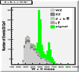
The main discovery channel for low-scale technicolor at the Tevatron is $\rho_{T}\rightarrow W^{\pm}\pi_{T}\rightarrow\ell^{\pm}\nu_{\ell}bq$, with at least one tagged $b$-jet. At the LHC, this channel is swamped by a $\bar{t}t$ background 100 times larger than at the Tevatron. There the discovery channels will be $WZ$, $\gamma W$ and $\gamma Z$, with the weak bosons decaying into charged leptons. In the TCSM each of these modes is dominated (generally $\mathrel{\hbox to0.0pt{\raise 2.20013pt\hbox{$>$}\hss}{\lower 2.20013pt\hbox{$\sim$}}}80\%$) by production of a single resonance:

$$\rho_{T}^{\pm}\rightarrow W^{\pm}Z^{0},\quad a_{T}^{\pm}\rightarrow\gamma W^{\pm},\quad\omega_{T}\rightarrow\gamma Z^{0}\,.$$ (2)

In Sects. 2-4, the PGS detector simulator [71] is used for our preliminary studies of these signals and their backgrounds. None of these LHC discovery modes involve observation of an actual technipion (other than the ones already observed, $W_{L}^{\pm}$ and $Z_{L}^{0}$). There are other strong-interaction scenarios of electroweak symmetry breaking (e.g., so-called Higgsless models in five dimensions [26, 72] and deconstructed models [15, 17, 16, 27]) which predict narrow vector and axial-vector resonances, but they do not decay to technipion-like objects. Therefore, observation of technipions in the final state is important for confirming LSTC as the mechanism underlying electroweak symmetry breaking. It is possible to do this at high luminosity with the decays $\rho_{T}^{\pm},\,a_{T}^{\pm}\rightarrow Z^{0}\pi_{T}^{\pm}\rightarrow\ell^{+}\ell^{-}bq$. This channel also provides the interesting possibility of observing both $\rho_{T}^{\pm}$ and $a_{T}^{\pm}$ in the same final state. This analysis, using ATLFAST [73], is summarized in Sect. 5 [74].

In addition to the discovery of narrow resonances in these channels, the angular distributions of the two-body final states in the techni-vector rest frame provide compelling evidence of their underlying technicolor origin. Because all the modes involve at least one longitudinally-polarized weak boson, the distributions are

$$\frac{d\sigma(\bar{q}q\rightarrow\rho_{T}^{\pm}\rightarrow W_{L}^{\pm}Z_{L}^{0})}{d\cos\theta},\;\;\frac{d\sigma(\bar{q}q\rightarrow\rho_{T}^{\pm}\rightarrow\pi_{T}^{\pm}Z_{L}^{0})}{d\cos\theta}\propto\sin^{2}\theta\,;$$ (3)

$$\frac{d\sigma(\bar{q}q\rightarrow a_{T}^{\pm}\rightarrow\gamma W_{L}^{\pm})}{d\cos\theta},\;\;\frac{d\sigma(\bar{q}q\rightarrow\omega_{T}\rightarrow\gamma Z_{L}^{0})}{d\cos\theta}\propto 1+\cos^{2}\theta\,.$$ (4)

It is fortunate that each of the two-electroweak-boson final states is dominated by a single technihadron resonance. Otherwise, because of the resonances’ expected closeness, it would likely be impossible to disentangle the different forms. Our simulations include these angular distributions.

For Les Houches, we concentrated on three TCSM mass points that cover most of the reasonable range of LSTC scales; they are listed in Table 2. In all cases, we assumed isospin symmetry, with $M_{\rho_{T}}=M_{\omega_{T}}$ and $M_{a_{T}}=1.1M_{\rho_{T}}$; also, the $\rho_{T}$ and $a_{T}$ constants describing coupling to their respective weak currents were taken equal; $\sin\chi=1/3$; $Q_{U}+Q_{D}=1$; $N_{TC}=4$ for the TC gauge group $SU(N_{TC})$; and $M_{V_{1,2,3}}=M_{A_{1,2,3}}=M_{\rho_{T}}$ for the LSTC mass parameters controlling the strength of $\rho_{T}$, $\omega_{T}$, $a_{T}$ decays to a transverse electroweak boson plus $\pi_{T}/W_{L}$ or $\rho_{T}$/$\omega_{T}$ [67, 68, 66]. Pythia [75] has been updated to include these and other LSTC processes, according to the rules of the TCSM. The new release and its description may be found at www.hepforge.org.

The simulations presented here, especially those using the PGS detector simulator [71], are preliminary and in many respects quite superficial. E.g., no attempt was made to optimize $S/B$ in the PGS studies. Nor did we carry out a serious analysis of statistical, let alone systematic, errors. Still, we believe the simulations establish the LHC’s ability to discover, or rule out, important signatures of low-scale technicolor. Beyond that, it is our intent that the present studies will stimulate more thorough ones by ourselves and by the ATLAS and CMS collaborations.

Case	$M_{\rho_{T}}=M_{\omega_{T}}$	$M_{a_{T}}$	$M_{\pi_{T}}$	$M_{\pi_{T}^{0\prime}}$		$\sigma(W^{\pm}Z^{0})$	$\sigma(\gamma W^{\pm})$	$\sigma(\gamma Z^{0})$	$\sigma(Z^{0}\pi_{T}^{\pm})$
A	300	330	200	400		110	168	19.2	158
B	400	440	275	500		36.2	64.7	6.2	88.6
C	500	550	350	600		16.0	30.7	2.8	45.4

Table 2: Masses (in GeV) and signal cross sections (in fb) for the lightest technihadrons for the three TCSM mass points in this study. Isospin symmetry is assumed. The $\pi_{T}^{0\prime}$ is an isosinglet, color-singlet technipion expected in TC models; we have assumed it so heavy that the $\rho_{T}$, $\omega_{T}$ and $a_{T}$ cannot decay to it. The cross sections combine contributions from $\rho_{T}$, $\omega_{T}$ and $a_{T}$, but tend to be dominated by a single resonance. Branching ratios of the $W$ and $Z$ to electrons and muons are included in all cross sections.

Background	Cross section (${\rm fb}$)	Comments
$WZ\rightarrow 3\ell+\nu$	430
$ZZ\rightarrow 4\ell$	52
$Z+\bar{b}b\rightarrow\ell^{+}\ell^{-}\leavevmode\nobreak\ \bar{b}b$	7600	$p_{T}(b)>15.0\ {\rm GeV},\ |\eta_{b}|<3.5$
$\bar{t}t\rightarrow 2\ell\leavevmode\nobreak\ 2\nu\leavevmode\nobreak\ \bar{b}b$	22,800	Pythia generator
$W\gamma\rightarrow\ell\nu\gamma$	2560	$p_{T}(\gamma)>40\ {\rm GeV},\ |\eta_{\gamma}|<3.5$
$W\,{\rm jet}\rightarrow\ell\nu\gamma$ (fake)	3180	$p_{T}({\rm jet})>40\ {\rm GeV},\ |\eta_{{\rm jet}}|<3.5$
		Includes 0.1% fake rate
$Z\gamma\rightarrow\ell^{+}\ell^{-}\gamma$	700	$p_{T}(\gamma)>40\ {\rm GeV},\ |\eta_{\gamma}|<3.5$
$Z\,{\rm jet}\rightarrow\ell^{+}\ell^{-}\gamma$ (fake)	315	$p_{T}({\rm jet})>40\ {\rm GeV},\ |\eta_{{\rm jet}}|<3.5$
		Includes 0.1% fake rate

Table 3: Backgrounds to the $W^{\pm}Z^{0}$, $\gamma W^{\pm}$ and $\gamma Z^{0}$ signals of low-scale technicolor. The generator is ALPGENv13 [77] unless indicated otherwise. Branching ratios of the $W$ and $Z$ to electrons and muons are included in the cross sections.

2 $\rho_{T}^{\pm}\rightarrow W_{L}^{\pm}Z_{L}^{0}\rightarrow\ell^{\pm}\nu_{\ell}\ell^{+}\ell^{-}$

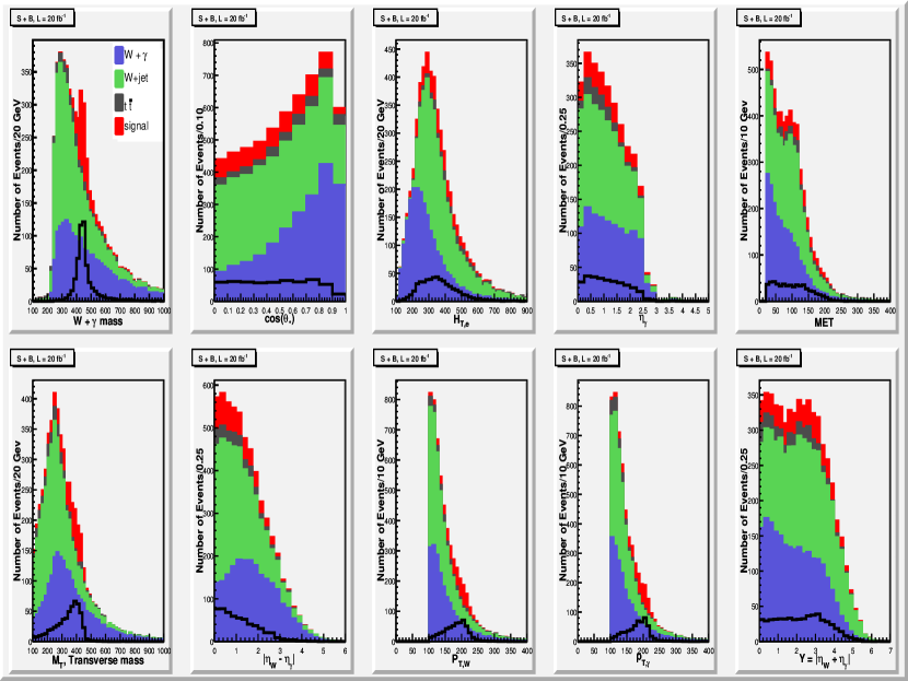
The cross sections for $\rho_{T}^{\pm}\rightarrow W_{L}^{\pm}Z_{L}^{0}$, including branching ratios to electrons and muons, are listed in Table 2. Signal events were generated with the updated Pythia [75]. The principal backgrounds are in Table 3, along with their generators and parton-level cuts. The ALPGEN backgrounds were passed through Pythia for showering and hadronization.

Events were selected which have exactly three leptons, electrons and/or muons, with two having the same flavor and opposite sign, $|\eta_{\ell}|<2.5$, at least one having $p_{T}>30\,{\rm GeV}$, and the others with $p_{T}>10\,{\rm GeV}$. No cut on $\kern 2.5pt\raise 0.77496pt\hbox{$/$}\kern-7.5ptE_{T}$ was applied in this analysis, though it may improve $S/B$ to do so. The $Z$ was reconstructed from two same-flavor, opposite-sign leptons with the smallest $|M_{\ell^{+}\ell^{-}}-M_{Z}|<7.8\,{\rm GeV}$. In reconstructing the $W$, ${\vec{p}}_{T}(\nu)=-\sum{\vec{\kern 2.5pt\raise 0.77496pt\hbox{$/$}\kern-7.5ptE_{T}}}$ was assumed, and the quadratic ambiguity in $p_{z}(\nu)$ was resolved in favor of the solution minimizing the opening angle between the neutrino and the charged lepton assigned to the $W$, as would be expected for a boosted $W$.

Figure 1 shows various distributions for case A with $p_{T}(W),\,p_{T}(Z)>50\,{\rm GeV}$ and $H_{T}({\rm jets})\equiv\sum E_{T}({\rm jet})<125\,{\rm GeV}$. The $H_{T}$ cut significantly reduces the $\bar{t}t$ background. The integrated luminosity is $10\,{\rm fb}^{-1}$, and a strong signal peak is clearly visible above background in the first panel. Fitting the peak to a Gaussian, its mass is $311\,{\rm GeV}$. Counting signal and background within twice the fitted resolution of $25\,{\rm GeV}$, only $\int{\cal L}dt=2.4\,{\rm fb}^{-1}$ is required for a $S/\sqrt{\smash[b]{S+B}}=5\,\sigma$ discovery of this resonance. Table 4 contains the final-state mass resolutions and $5\,\sigma$ discovery luminosities for the two-electroweak-boson modes considered here. The poorer resolution in the $WZ$ and $\gamma W$ channels is due to the $\kern 2.5pt\raise 0.77496pt\hbox{$/$}\kern-7.5ptE_{T}$ resolution.

$WZ$	$M_{\rm peak}$ $({\rm GeV})$	$\sigma\ ({\rm GeV})$	${\cal L}_{\rm min}\,({\rm fb}^{-1})$	$p_{T}$ cut
A	311	25.6	2.4	$p_{T}(W,Z)>50\ {\rm GeV}$
B	414	34.5	7.2	$p_{T}(W,Z)>75\ {\rm GeV}$
C	515	41.0	14.7	$p_{T}(W,Z)>75\ {\rm GeV}$
$\gamma W$	$M_{\rm peak}$ $({\rm GeV})$	$\sigma\ ({\rm GeV})$	${\cal L}_{\rm min}\,({\rm fb}^{-1})$	$p_{T}$ cut
A	328	31.2	2.3	$p_{T}(\gamma,W)>75\ {\rm GeV}$
B	439	39.1	4.5	$p_{T}(\gamma,W)>100\ {\rm GeV}$
C	547	39.3	7.8	$p_{T}(\gamma,W)>125\ {\rm GeV}$
$\gamma Z$	$M_{\rm peak}$ $({\rm GeV})$	$\sigma\ ({\rm GeV})$	${\cal L}_{\rm min}\,({\rm fb}^{-1})$	$p_{T}$ cut
A	299	7.3	16.8	$p_{T}(\gamma,Z)>80\ {\rm GeV}$
B	398	9.4	45.5	$p_{T}(\gamma,Z)>110\ {\rm GeV}$
C	498	12.0	97.2	$p_{T}(\gamma,Z)>150\ {\rm GeV}$

Table 4: PGS simulation data for the spin-one technihadrons decaying to a pair of electroweak gauge bosons. A simple Gaussian fit is made to determine the mass and width of the resonance; signal and background events are counted within $\pm 2\,\sigma$ of the peak value to determine the minimum luminosity needed for $S/\sqrt{\smash[b]{S+B}}=5\,\sigma$.

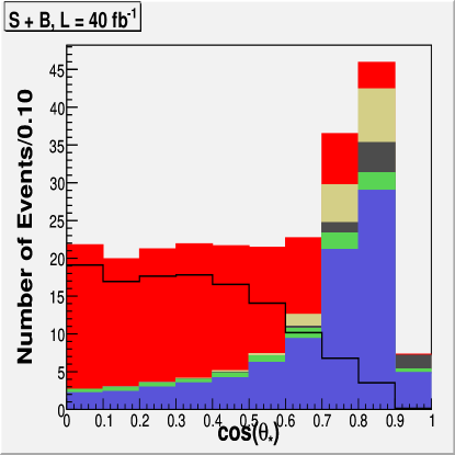
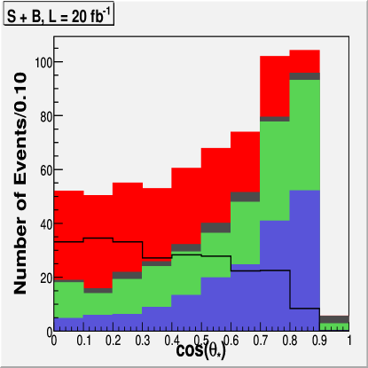
The second panel in Fig. 1 shows the total and signal $WZ$ angular ($|\cos\theta|$) distribution. The distribution is folded since the signal and $WZ$ background are even functions of $\cos\theta$. The total distribution reflects the forward-backward peaking of the standard $WZ$ production. The signal distribution (open black histogram) is much flatter than the expected $\sin^{2}\theta$, presumably because of poorly-fit $W$’s and their effect on determining $M_{WZ}$ and the $WZ$ rest frame. To remedy this, we take advantage of the LSTC technihadrons’ very small widths and require $280<M_{WZ}<340\,{\rm GeV}$; see Fig. 2. The signal distribution now has the expected $\sin^{2}\theta$ shape. The remaining large background at $|\cos\theta|\mathrel{\hbox to0.0pt{\raise 2.20013pt\hbox{$>$}\hss}{\lower 2.20013pt\hbox{$\sim$}}}0.7$ can be fit and subtracted by measuring the angular distribution in the sidebands $220\mathrel{\hbox to0.0pt{\raise 2.20013pt\hbox{$<$}\hss}{\lower 2.20013pt\hbox{$\sim$}}}M_{WZ}\mathrel{\hbox to0.0pt{\raise 2.20013pt\hbox{$<$}\hss}{\lower 2.20013pt\hbox{$\sim$}}}280\,{\rm GeV}$ and $340\mathrel{\hbox to0.0pt{\raise 2.20013pt\hbox{$<$}\hss}{\lower 2.20013pt\hbox{$\sim$}}}M_{WZ}\mathrel{\hbox to0.0pt{\raise 2.20013pt\hbox{$<$}\hss}{\lower 2.20013pt\hbox{$\sim$}}}400\,{\rm GeV}$. We believe that $10\,{\rm fb}^{-1}$ is sufficient to distinguish this angular distribution from $1+\cos^{2}\theta$, but detailed fitting is required to confirm this; see Ref. [78].

Figure 1: Signal and background distributions of a $300\,{\rm GeV}$ $\rho_{T}^{\pm}\rightarrow W^{\pm}Z^{0}\rightarrow\ell^{\pm}\nu_{\ell}\ell^{+}\ell^{-}$ for $10\,{\rm fb}^{-1}$ at the LHC; $p_{T}(W,Z)>50\,{\rm GeV}$ and $H_{T}({\rm jets})<125\,{\rm GeV}$. The open black histograms are the signal contributions.

Figure 2: $WZ$ angular distribution of the signal and backgrounds for a $300\,{\rm GeV}$ $\rho_{T}^{\pm}\rightarrow W^{\pm}Z^{0}\rightarrow\ell^{\pm}\nu_{\ell}\ell^{+}\ell^{-}$ for $10\,{\rm fb}^{-1}$ at the LHC; $280<M_{WZ}<340\,{\rm GeV}$; other cuts are listed in the text. The color code is given in Fig. 1.

Figure 3: $WZ$ angular distributions of the signal and backgrounds for $\rho_{T}^{\pm}\rightarrow W^{\pm}Z^{0}\rightarrow\ell^{\pm}\nu_{\ell}\ell^{+}\ell^{-}$ Left: $M_{\rho_{T}}=400\,{\rm GeV}$ with $380<M_{WZ}<440\,{\rm GeV}$ for $40\,{\rm fb}^{-1}$. Right: $M_{\rho_{T}}=500\,{\rm GeV}$ with $480<M_{WZ}<540\,{\rm GeV}$ for $80\,{\rm fb}^{-1}$. Other cuts are listed in the text. The color code is given in Fig. 1.

Figure 4: Fit of the signal and background $WZ$ invariant mass distribution, for case C with $50\,{\rm fb}^{-1}$, in ATLAS. Red curves represent the signal resonances, blue the backgrounds, and green the total [78].

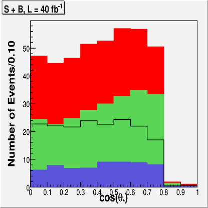
The $|\cos\theta|$ distribution in the $\rho_{T}$-resonance region is shown in Fig. 3 for cases B ($M_{\rho_{T}}=400\,{\rm GeV}$) and C ($500\,{\rm GeV}$). The $p_{T}(W,Z)$ cuts of 75 and $100\,{\rm GeV}$ were chosen to accept signal data over the same $\cos\theta$ range, 0.0–0.9, as in Case A. The luminosities of 40 and $80\,{\rm fb}^{-1}$ were chosen to give roughly the same statistics. For the higher luminosities, the effects of pile-up on calorimetry and tracking were not considered.

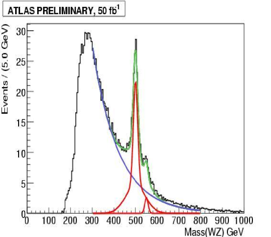
Finally, for the $50\,{\rm GeV}$ splitting used in case C, it appears possible to see $\rho_{T}^{\pm}$ and $a_{T}^{\pm}$ as separate peaks in the $M_{WZ}$ distribution. This was studied in Refs. [78, 79]. With cuts similar to those used above (except that $p_{T}(W,Z)>50\,{\rm GeV}$) a simulation [78] using ATLFAST was performed. The result is seen in Fig. 4 where a luminosity of $50\,{\rm fb}^{-1}$ was assumed. The $\rho_{T}$ and $a_{T}$ were modeled as Gaussian distributions and the background above $300\,{\rm GeV}$ as a falling exponential. The $a_{T}$ appears as a high-mass shoulder. The CMS analysis finds a similar result [79]. Both $\rho_{T}$ and $a_{T}$ can be observed and a $5\,\sigma$ (combined) discovery achieved with luminosity $\simeq 9.5\,{\rm fb}^{-1}$ provided that data is reasonably described by the simulated $\kern 2.5pt\raise 0.77496pt\hbox{$/$}\kern-7.5ptE_{T}$ resolution.

3 $a_{T}^{\pm}\rightarrow\gamma W_{L}^{\pm}$

Figure 5: Signal and background distributions of a $440\,{\rm GeV}$ $a_{T}^{\pm}\rightarrow\gamma W^{\pm}\rightarrow\gamma\ell^{\pm}\nu_{\ell}$ for $20\,{\rm fb}^{-1}$ at the LHC; $p_{T}(\gamma,W)>100\,{\rm GeV}$ and $\kern 2.5pt\raise 0.77496pt\hbox{$/$}\kern-7.5ptE_{T}>20\,{\rm GeV}$. The open black histograms are the signal contributions.

The axial-vector isovector $a_{T}$ is a new addition to the TCSM framework, motivated by the arguments that the $S$ parameter problem of technicolor is ameliorated if $\rho_{T}$ and $a_{T}$ are nearly degenerate and have nearly the same couplings to the vector and axial-vector weak currents.

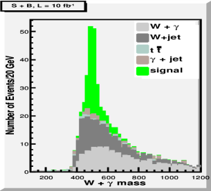
On account of space limitation, we show here only the results of PGS simulation of Case B, for which $M_{a_{T}}=440\,{\rm GeV}$. For the decays to a pair of electroweak bosons considered in this report, $\sigma(a_{T}\rightarrow\gamma W)B(W\rightarrow e/\mu\,\nu)$ are the largest; it is $65\,{\rm fb}$ in case B. Signal and background events were generated with $p_{T}(\gamma)>40\,{\rm GeV}$. As noted, the discovery search could impose a higher threshold. Events were selected with exactly one lepton, having $p_{T}>10\,{\rm GeV}$ and $|\eta|<2.5$. Distributions are displayed in Fig. 5, in which $\kern 2.5pt\raise 0.77496pt\hbox{$/$}\kern-7.5ptE_{T}>20\,{\rm GeV}$ and $p_{T}(\gamma),\,p_{T}(W)>100\,{\rm GeV}$. The principal backgrounds are in Table 3. A ${\rm jet}\rightarrow\gamma$ fake rate of $10^{-3}$ was assumed for $W+{\rm jet}$ [37]. Another possible background, $\gamma+{\rm jet}$ where the jet fakes a lepton, is negligible after the $\kern 2.5pt\raise 0.77496pt\hbox{$/$}\kern-7.5ptE_{T}$ cut. The luminosity of $20\,{\rm fb}^{-1}$ was chosen to give reasonable statistics for the signal’s angular distribution. Consequently, the $a_{T}$ resonant peak has a significance of $10\,\sigma$.

It is clear from these distributions that the backgrounds are a more severe impediment to observing the signal’s angular distribution ($1+\cos^{2}\theta$) than they were in the case of $\rho_{T}\rightarrow WZ$. In particular, there is no obvious cut to remove them other than one on $M_{\gamma W}$. The result of requiring $420<M_{\gamma W}<460\,{\rm GeV}$ is in Fig. 6. Even though the signal’s expected forward-backward excesses are eliminated by the $p_{T}(\gamma)$ cut, this clearly is a flatter distribution than the $\sin^{2}\theta$ ones above. As in that case, subtracting the background by measuring the sidebands should reveal the signal. Careful fitting to see that it is consistent with $1+\cos^{2}\theta$ after cuts is work for the future.

Figure 6: Angular distributions for the signal and backgrounds for a $440\,{\rm GeV}$ $a_{T}^{\pm}\rightarrow\gamma W^{\pm}$ with $420<M_{\gamma W}<460\,{\rm GeV}$ (left) and a $300\,{\rm GeV}$ $\omega_{T}\rightarrow\gamma Z^{0}$ with $290<M_{\gamma Z}<310\,{\rm GeV}$ (right) at the LHC; other cuts are listed in the text. The luminosities are 20 and $40\,{\rm fb}^{-1}$, respectively. The color codes are given in Figs. 5 and 7.

4 $\omega_{T}\rightarrow\gamma Z_{L}^{0}$

The $\omega_{T}$ is as important to find as the $\rho_{T}$, with which it is expected to be nearly degenerate, and the $a_{T}$. Yet it is the most challenging to see of the light techni-vectors. At the Tevatron, the primary discovery mode is $\omega_{T}\rightarrow\gamma\pi_{T}^{0}\rightarrow\gamma b\bar{b}$. Backgrounds to this may make this channel difficult at the LHC; studies need to be done! Two other channels have much lower branching ratios, but are much cleaner: $\omega_{T}\rightarrow\gamma Z_{L}^{0}\rightarrow\gamma\ell^{+}\ell^{-}$ and $\omega_{T}\rightarrow\ell^{+}\ell^{-}$. We discuss the first of these in this section.

As with the $a_{T}$ search just described, the main backgrounds to $\omega_{T}\rightarrow\gamma Z^{0}$ are standard $Z^{0}+\gamma$ and $Z+\,{\rm jet}(\rightarrow\gamma)$ production. The $\omega_{T}$ signal, however, is about 10 times smaller than the $a_{T}$ one (see Table 2), so considerably higher luminosities are required to see a significant signal peak and the characteristic $1+\cos^{2}\theta$ distribution. Here we discuss the PGS simulation for case A, in which $M_{\omega_{T}}=300\,{\rm GeV}$. Events were selected with two same-flavor, opposite-sign leptons, each having $p_{T}>10\,{\rm GeV}$ and rapidity $|\eta|<2.5$. The leptons were required to satisfy $|M_{\ell^{+}\ell^{-}}-M_{Z}|<7.8\,{\rm GeV}$. Distributions are shown in Fig. 7 for a luminosity of $40\,{\rm fb}^{-1}$ and for $p_{T}(\gamma),\,p_{T}(Z)>80\,{\rm GeV}$. Note the much better final-state mass resolution than for $\rho_{T}\rightarrow WZ$ and $a_{T}\rightarrow\gamma W$. The significance of the signal peak is about $8\,\sigma$; the high luminosity is needed to accumulate statistics for the angular distribution.

To expose the angular distribution, we take advantage of the superior $\gamma Z$ mass resolution and impose a tight cut on $M_{\gamma Z}$ of $300\pm 10\,{\rm GeV}$. The result is in Fig. 6. Because of the more stringent $p_{T}$ cuts, the data above $|\cos\theta|>0.8$ are lost. While quite acceptable, the angular distribution’s signal-to-background is not as favorable as it was for $a_{T}\rightarrow\gamma W$. As in that case, detailed fitting beyond our scope is needed to determine how well the measured distribution fits the expectation. And, as there, the backgrounds can be subtracted by measuring the angular distribution in sidebands.

Figure 7: Signal and background distributions of a $300\,{\rm GeV}$ $\omega_{T}\rightarrow\gamma Z^{0}\rightarrow\gamma\ell^{+}\ell^{-}$ for $40\,{\rm fb}^{-1}$ at the LHC; $|M_{\ell^{+}\ell^{-}}-M_{Z}|<7.8\,{\rm GeV}$ and $p_{T}(\gamma,Z)>80\,{\rm GeV}$. The open black histograms are the signal contributions.

5 $\rho_{T}^{\pm},\,a_{T}^{\pm}\rightarrow Z^{0}\pi_{T}^{\pm}\rightarrow\ell^{+}\ell^{-}bq$

Even if narrow resonances in the $WZ$, $\gamma W$ and $\gamma Z$ channels are found as described above at the LHC, all with nearly the same mass and with the expected angular distributions, it will remain essential to discover a technipion to cement the technicolor interpretation of these states. In this section we present an analysis of $\rho_{T}^{\pm}\rightarrow Z^{0}\pi_{T}^{\pm}$ carried out for the ATLAS detector [74]. The large backgrounds to this signal require large luminosity. On the other hand, for the masses assumed here, this channel has the extra advantage that the rate for $a_{T}^{\pm}\rightarrow Z_{\perp}^{0}\pi_{T}^{\pm}$ is only 2–4 times smaller than for $\rho_{T}^{\pm}\rightarrow Z_{L}^{0}\pi_{T}^{\pm}$, creating another opportunity for observing both resonant peaks in the same (well, similar) final state.

As noted, $\pi_{T}$ are expected to decay into the heaviest fermion-antifermion flavors kinematically allowed. For the range of $M_{\pi_{T}}$ considered here, this implies $\pi_{T}^{+}\rightarrow t\bar{b}$ and $\pi_{T}^{0}\rightarrow\bar{b}b$ or $\bar{t}t$ are dominant. Actually, something like topcolor-assisted technicolor [69] is needed to produce $m_{t}\simeq 175\,{\rm GeV}$, and this implies that the coupling of $\pi_{T}$ to $t$-quarks is suppressed by a factor of about $m_{b}/m_{t}$ from its naive value. Thus, while the $\pi_{T}^{+}$ considered here is massive enough to decay to $t\bar{q}$, it should still have an appreciable branching fraction to $c\bar{b}$ and $u\bar{b}$. The latter are the decay channels considered here. It will be interesting to consider the $t\bar{q}$ modes. However, they are not yet included in Pythia and, therefore, $B(\pi_{T}^{+}\rightarrow b\bar{q})=0.87$ in the simulation reported here. This branching ratio may decrease substantially when the top modes are included. That would change the search strategy, but we expect that $\pi_{T}^{+}$ can be seen in $t\bar{q}$ as well.

Figure 8: Left: $M_{\rho_{T}}-M_{\pi_{T}}$ and $M_{a_{T}}-M_{\pi_{T}}$ for cases A, B, C in ATLAS. Right: $M_{\rho_{T},\,a_{T}}-M_{\pi_{T}}$ vs. $M_{\pi_{T}}$ signal and background events per $2\times 10\,{\rm GeV}^{2}$ per $100\,{\rm fb}^{-1}$ for case A [74].

The signal cross sections are $\sigma(pp\rightarrow\rho_{T}^{\pm},\,a_{T}^{\pm}\rightarrow Z^{0}\pi_{T}^{\pm})B(Z^{0}\rightarrow\ell^{+}\ell^{-})=(99,\,59)$ (A), $(71,\,17)$ (B), and $(37,\,9)\,{\rm fb}$ (C), where the two numbers are approximately the $\rho_{T}^{\pm}$ and $a_{T}^{\pm}$ contributions. The principal backgrounds and their leading-order cross sections are: $\bar{t}t$ ($500\,{\rm pb}$) and, including the branching ratio of $Z^{0}$ to $e^{+}e^{-}$ and $\mu^{+}\mu^{-}$, $Z^{0}jj$ ($344\,{\rm pb}$), $Z^{0}b\bar{b}$ ($56\,{\rm pb}$) and $Z^{0}bj$ ($11\,{\rm pb}$). See Ref. [74] for generation details. The ATLAS detector simulation used ATLFAST [73]. An additional factor of 90% was applied to the simulation for lepton identification efficiency. The $b$-jet tag efficiency used was 50%; this corresponds to a light-jet mistag rate of 1% and a $c$-jet mistag rate of 10%.

To satisfy ATLAS trigger and high-luminosity ($100\,{\rm fb}^{-1}$ per year) running conditions, events were preselected with (1) two same-flavor opposite-sign leptons with $p_{T}>20\,{\rm GeV}$ and (2) at least one $b$-tagged jet and one non-$b$-tagged jet, both with $p_{T}>20\,{\rm GeV}$; the two highest-$p_{T}$ jets satisfying these conditions are the $\pi_{T}$-candidate jets. For the $\rho_{T}^{\pm}$, these selections resulted in 548 (A), 382 (B) and 184 (C) signal events per $100\,{\rm fb}^{-1}$. For the $a_{T}^{\pm}$, there were 297 (A), 117 (B) and 34 (C) events. The total background event numbers, dominated by $Zjj$ and $Zb\bar{b}$, were: (6930, 10670) (A), (7505, 6285) (B) and (3015, 2550) (C). Here, the first number in each pair refers to $\rho_{T}$ and the second to $a_{T}$; the background is the number of events in an elliptical region in $M_{\pi_{T}}$–$(M_{\rho_{T},\,a_{T}}-M_{\pi_{T}})$ space centered at the mean and with widths corresponding to $1.5\,\sigma$.

The following cuts were then applied to optimize the signal significances: (1) $\kern 2.5pt\raise 0.77496pt\hbox{$/$}\kern-7.5ptE_{T}<35\,{\rm GeV}$ to suppress $t\bar{t}$; (2) the highest-$p_{T}$ jet had $p_{T}>80$ (A), 115 (B), $150\,{\rm GeV}$ (C); (3) the second highest-$p_{T}$ jet had $p_{T}>65$ (A), 80 (B), $100\,{\rm GeV}$ (C); (4) there is exactly one $b$-tagged jet; and (5) $M_{\ell^{+}\ell^{-}}=91\pm 5\,{\rm GeV}$. After these cuts, the number of remaining signal events is (344, 215) (A), (242,75) (B) and (126,21) (C) for ($\rho_{T}^{\pm},\,a_{T}^{\pm}$).The backgrounds under these signals are (403,900) (A), (346,242) (B) and (96,69) (C). For the parameters used in this simulation, then, only in case C is the $a_{T}$ not observable in the $Z\pi_{T}$ channel in $100\,{\rm fb}^{-1}$.

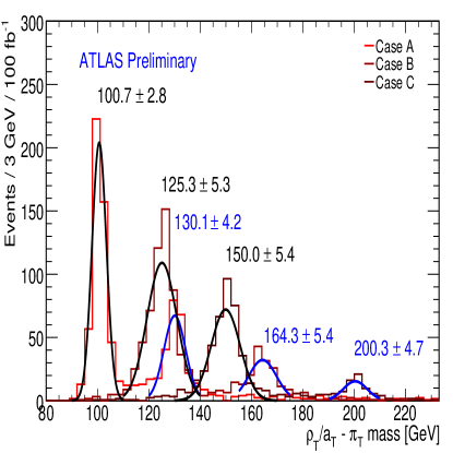
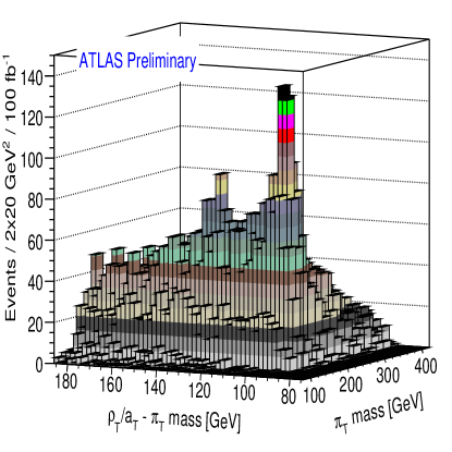
The resolution in $M_{\pi_{T}}$ varies from 16 to $23\,{\rm GeV}$ and in $M_{\rho_{T},\,a_{T}}$ from 19 to $30\,{\rm GeV}$. Most of the error comes from the $\pi_{T}$ jets’ energy measurements. Therefore, much of it cancels in $Q=M_{\rho_{T},\,a_{T}}-M_{\pi_{T}}$. This is shown on the left in Fig. 8, where the resolution in this difference ranges from 3 to $5\,{\rm GeV}$. This sharpness will facilitate the discovery of $\rho_{T},\,a_{T}\rightarrow Z\pi_{T}$ and other technivector-to-technipion decays. The signals and background for case A are on the right in Fig. 8. The twin peaks stand out dramatically (looking rather like Boston’s Back Bay).

In summary: For the TCSM parameters used here, there should be no difficulty seeing $\rho_{T}^{\pm}$ and $a_{T}^{\pm}$ in the $Z^{0}\pi_{T}^{\pm}$ channel in case A, and the $\rho_{T}$ and a strong indication of the $a_{T}$ in case B. In case C, only $\rho_{T}^{\pm}\rightarrow Z^{0}\pi_{T}^{\pm}$ can be seen in $100\,{\rm fb}^{-1}$. The minimal cross sections (times $B(Z\rightarrow e^{+}e^{-}\,/\mu^{+}\mu^{-})$) and luminosities required to see the $\rho_{T}^{\pm}$ and $a_{T}^{\pm}$ signals at $5\,\sigma$ significance are in Table 5.

peak	A	B	C		A	B	C
$\rho_{T}^{\pm}$	29	28	14		8.3	15	15
$a_{T}^{\pm}$	41	18	18		48	106	390

Table 5: Minimal cross-section times branching fractions (in fb, left) and minimal luminosities (in ${\rm fb}^{-1}$, right) required for $5\,\sigma$ significance in cases A, B, C.

6 CONCLUSIONS AND OUTLOOK

Low-scale technicolor (with $N_{D}={\cal O}(10)$ isodoublets transforming as $SU(N_{TC})$ fundamentals) is a well-motivated scenario for strong electroweak symmetry breaking with a walking TC gauge coupling. The Technicolor Straw-Man framework provides the simplest phenomenology of this scenario by assuming that the lightest technihadrons — $\rho_{T}$, $\omega_{T}$, $a_{T}$ and $\pi_{T}$ — and the electroweak gauge bosons can be treated in isolation. This framework is now implemented in Pythia.

We used Pythia and (mainly) the generic detector simulator PGS to study the final-state mass peaks and angular distributions for the LSTC discovery channels at the LHC: $\rho_{T}^{\pm}\rightarrow W^{\pm}Z^{0}$, $a_{T}^{\pm}\rightarrow\gamma W^{\pm}$ and $\omega_{T}\rightarrow\gamma Z^{0}$, with leptonic decays of the weak bosons. We also carried out an ATLFAST simulation for $\rho_{T}^{\pm},\,a_{T}^{\pm}\rightarrow Z^{0}\pi_{T}^{\pm}\rightarrow\ell^{+}\ell^{-}b\,{\rm jet}$. The results are very promising. For the fairly generic TCSM parameters chosen, the technivector mesons can be discovered up to about 500–$600\,{\rm GeV}$ in the two-gauge boson modes, usually with a few to a few tens of ${\rm fb}^{-1}$. The angular distributions, dispositive of the underlying technicolor dynamics, can be discerned with a few tens to $100\,{\rm fb}^{-1}$ (except for a higher mass $\omega_{T}\rightarrow\gamma Z^{0}$). Taking advantage of the superb resolutions in $Q=M_{\rho_{T},a_{T}}-M_{\pi_{T}}$ and $M_{\ell^{+}\ell^{-}}$ for $\rho_{T},\,a_{T}\rightarrow Z\pi_{T}\rightarrow\ell^{+}\ell^{-}b\,{\rm jet}$, both resonances and the technipion can be seen for $M_{\rho_{T}}\mathrel{\hbox to0.0pt{\raise 2.20013pt\hbox{$<$}\hss}{\lower 2.20013pt\hbox{$\sim$}}}500\,{\rm GeV}$ and $M_{a_{T}}\mathrel{\hbox to0.0pt{\raise 2.20013pt\hbox{$<$}\hss}{\lower 2.20013pt\hbox{$\sim$}}}400\,{\rm GeV}$.

Still, these studies just scratch the surface of what can and needs to be done to gauge the potential of the ATLAS and CMS detectors for discovering and probing low-scale technicolor. Simulating detector response to the signals and backgrounds of the relatively simple processes we considered requires considerably more sophistication, in both depth and breadth, than we have been able to deploy. Issues such as the accuracy with which technivector masses and decay angular distributions can be determined as a function of luminosity are especially important. While we believe that the TCSM parameters — $\sin\chi$, $Q_{U}+Q_{D}$, $M_{\pi_{T}}$, $M_{V_{i}}$ and $M_{A_{i}}$, $N_{TC}$ — we chose are reasonable, relative branching fractions can be fairly sensitive to them, as Table 1 indicates [68]. It would be valuable to reconsider the processes examined here for a range of these parameters. Finally, there are other modes we have not been able to consider but which are nevertheless of considerable interest. Two outstanding examples are $\rho_{T}^{0},\,\omega_{T},\,a_{T}^{0}\rightarrow\ell^{+}\ell^{-}$ and $\omega_{T},\,\rho_{T}^{0}\rightarrow\gamma\pi_{T}^{0}\rightarrow\gamma\bar{b}b$. Thus, the main goal of our Les Houches studies, as it is for the other “Beyond the Standard Model” ones started at Les Houches, is to motivate the ATLAS and CMS collaborations to broaden the scope of their searches for the origin and dynamics of electroweak symmetry breaking.

“Faith” is a fine invention

When Gentlemen can see —

But Microscopes are prudent

In an Emergency.

— Emily Dickinson, 1860

ACKNOWLEDGEMENTS

We thank the organizers and conveners of the Les Houches workshop, “Physics at TeV Colliders”, for a most stimulating meeting and for their encouragement in preparing this work. We are especially grateful to Steve Mrenna for updating Pythia to include all the new TCSM processes. We also thank participants, too many to name, for many spirited discussions. Lane and Martin are indebted to Laboratoire d’Annecy-le-Vieux de Physique des Particules (LAPP) and Laboratoire d’Annecy-le-Vieux de Physique Theorique (LAPTH) for generous hospitality and support throughout the course of this work. Part of this work has been performed within the ATLAS Collaboration (Azuelos and Ferland; Black) and the CMS Collaboration (Bose), and we thank members of both collaboration for helpful discussions. We have made use of their physics analysis framework and tools which are the result of collaboration-wide efforts. This research was supported in part by NSERC, Canada (Azuelos and Ferland) and the U.S. Department of Energy under Grants DE-FG02-91ER40654 (Black), DE-FG02-91ER40688 (Bose), DE-FG02-97ER41022 (Gershtein), DE-FG02-91ER40676 (Lane), and DE-FG02-92ER40704 (Martin).

Part 5 Technivectors at the LHC

J. Hirn, A. Martin and V. Sanz

1 INTRODUCTION:

As was emphasized in the Les Houches non-SUSY BSM working group, very few LHC simulations of dynamical electroweak symmetry breaking (DEWSB) scenarios are available. In order to remedy this situation, Les Houches 2007 called for an effective description of strong interactions, flexible enough to interpolate between some known models of resonance interactions in 4D or 5D, yet economical enough to have a tractable parameter space. Ultimately, such a framework could play the same role for strong interactions as was played by minimal Supergravity (mSUGRA) for the case of SUSY: simplifying assumptions reduce the number of parameters from $\mathcal{O}(100)$ down to a few, enabling a slew of phenomenological studies.

As a step towards an effective DEWSB description, we present a flexible yet manageable model of interactions between spin-1 resonances and the Standard Model (without Higgs) using the framework of Holographic Technicolor (HTC) [64]. In HTC the number of parameters in the effective lagrangian of resonance interactions is reduced by deriving the interactions from a precursor 5D lagrangian, as suggested by the AdS/CFT correspondence [80, 81]. In practice, we see no reason to be constrained by a strict 5D formulation [82]: we simply model interactions between 4D resonances, but resort to 5D techniques to compute the parameters.

HTC is similar to Higgsless [17] models, but contains deviations from pure AdS 5D geometry in the form of effective warp factors that differ for the various fields. These warp factors are a departure from true 5D modelling [82] but they are motivated by the requirement of small deviations from the SM in the gauge sector (oblique corrections [64], and cubic couplings, see below). With nonstandard 5D geometry we achieve a different resonance spectrum from rescaled QCD, confirming and building upon previous 4D results [83, 56, 62].

We also refrain from modelling the fermions in the extra-dimension, as this would not reduce the number of parameters: in the present study, the couplings of fermions to resonances $g_{ffV}$ are free parameters, set to pass experimental constraints, while the couplings of fermions to $W,Z$ are assumed to exactly obey SM relations. This can be relaxed in the future.

In sections 2 and 3 we present the basics of HTC parameterization and the constraints on its parameter space. In sections 4 and 5 we describe some LHC signals using a MadGraph [35]/BRIDGE [84] implementation of HTC. In the future we hope to provide a more complete package to allow further study.

2 HOLOGRAPHIC TECHNICOLOR:

In HTC, as in Higgsless models, the SM $SU(2)_{\rm w}$ and $U(1)_{{\rm em}}$ gauge fields are the lightest Kaluza-Klein (KK) states of 5D $SU(2)_{L}\otimes SU(2)_{R}$ gauge fields. The higher KK excitations of the same 5D fields are interpreted as new spin-1 resonances. Provided they are light enough, these spin-1 resonances assist in unitarizing $WW$ scattering in the absence of a Higgs.

The masses and interactions of the resonances are dictated by the geometry of the 5th dimension, which is set by a warp factor $w(z)$. The warp factor appears in the 5D metric $ds^{2}=w(z)^{2}(dx^{2}-dz^{2})$, where the extra coordinate $z$ is restricted to the interval $l_{0}\leqslant z\leqslant l_{1}$. Instead of a single warp factor, in HTC we allow the axial ($A$) and vector ($V$) combinations of 5D gauge fields to feel different backgrounds. Specifically we define $w_{X}=(l_{0}/z)\exp\left(\frac{o_{X}}{2}\left(\frac{z-l_{0}}{l_{1}}\right)^{4}\right)$, $X=A,V$. The power $4$ in $(z/l_{1})^{4}$ was based on walking technicolor arguments [22], but is irrelevant for LHC phenomenology: one can absorb the effect of a different power in the $o_{X}$ value. Pure AdS geometry corresponds to $o_{V,A}=0$. Choosing boundary conditions that preserve only $U(1)_{{\rm em}}$ leads to a massless photon, and light $W,Z$ compared to the resonances. Although 5D provides a tower of resonances, we restrict our study to the lightest two triplets of resonances $(W_{1,2}^{\pm},Z_{1,2})$. These resonances are narrow, $\Gamma\sim{\rm GeV}$ .

While we assume the strong interactions themselves to be parity symmetric , the coupling to the EW sector (set by boundary conditions) leads to physical mass eigenstates that are an admixture of axial and vector components. The mass splitting between resonances is directly affected by nonzero $o_{V},o_{A}$, as are their couplings. Specifically, the permutation symmetry among triboson couplings does not hold: for $B,C,D$ representing three different HTC spin-1 particles (including $\gamma,W^{\pm},Z$)

$$g_{BCD}(\partial_{[\mu}B^{-}_{\nu]}C^{+\mu}D^{0\nu})+g_{BCD2}(\partial_{[\mu}C^{+}_{\nu]}D^{0\mu}B^{-\nu})+g_{BCD3}(\partial_{[\mu}D^{0}_{\nu]}B^{-\mu}C^{+\nu}),$$ (1)

we find $g_{BCD}\neq g_{BCD2}\neq g_{BCD3}$. We modified both MadGraph and BRIDGE accordingly.

In summary, the HTC description is very economical. The remaining free parameters are: the size of the ED ($l_{1}$), which sets the overall mass scale for the new resonances, $M\sim 1/l_{1}$, the amount of departure from AdS geometry ($o_{V,A}$) and the coupling of the resonances to SM fermions ($g_{ffV}$).

3 PARAMETER CONSTRAINTS:

In a pure-AdS model ($o_{V}=o_{A}=0$), consistency with precision electroweak measurements (especially the $S$ parameter) requires fermiophobic resonance couplings, $g_{ffV}\approx 0$ [27]. This is not true in HTC, where we find regions of parameter space in which $S$ is small due to cancellations between resonance multiplets. In the lefthand side of Fig. 1, we show the line along which oblique corrections cancel. Along that line, the lightest two resonances are separated by only $\gtrsim 100\ {\rm GeV}$, though the exact spacing depends on the full set of 5D parameters. The mass separation between the $W_{1}$ and $W_{2}$ greatly impacts the phenomenology, as we see in section 4.

Figure 1: Lefthand side: line of $S=0$ in the $o_{A},o_{V}$ plane with the two sample points on the $o_{A}=0$ axis. Righthand side: setting $o_{A}=0$ and $M_{W_{1}}=500\ {\rm GeV}$, value of the trilinear gauge coupling $g_{1}^{Z}$ as a function of $o_{V}$. The two horizontal lines correspond to the 1$\sigma$ bounds [85].

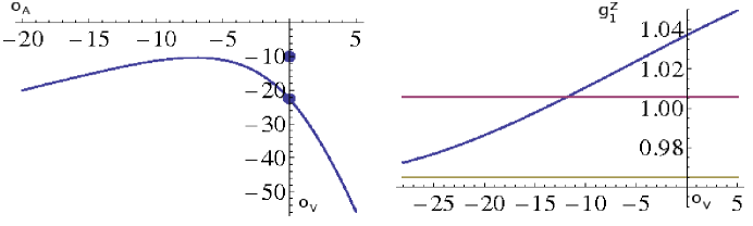
Having narrowed down the $o_{V},o_{A}$ region of interest, for the present study we simply set the couplings of fermions to the $W,Z$ to follow the SM relations, and take the couplings $g_{ffV}$ of fermions to resonances as free parameters. The $g_{ffV}$ are still constrained by direct $Z^{\prime},W^{\prime}$ Tevatron cross section bounds [86, 87] and by contact interaction limits [88, 85]. In any particular HTC model, one must also check that the resonances do not disrupt the measured Tevatron diboson cross sections [89, 90] and high $p_{T,Z},p_{T,\gamma}$ distributions [89, 91].

For a given resonance mass, the geometry parameters $o_{V},o_{A}$ are constrained by LEP limits on anomalous triboson couplings [85], as depicted in the righthand side of Fig. 1. As a first application of the HTC framework we now summarize the LHC signals of the two HTC points indicated in Fig. 1. For the details of the analysis, see Ref. [92].

4 S-CHANNEL PRODUCTION:

Because HTC resonances need not be fermiophobic they can be produced as $s$-channel resonances. In our setup, $WZ$ is the dominant decay mode for charged resonances , therefore in Ref. [92] we considered the mode:

$${\rm pp}\rightarrow W^{\pm}_{1,2}\rightarrow W^{\pm}Z,W^{\pm}Z\rightarrow 3\ell+\nu$$ (2)

In figure (2) we show the invariant mass distributions in the $W^{\pm}Z$ channel for the two sample HTC points in [92]. For these points we have set the values of $g_{ffV}$ to be compatible with Tevatron-LEP limits and yet both resonances could be discovered within the first few ${\rm fb}^{-1}$ at the LHC. These points are just an example, chosen because they have large signals at the LHC.

Figure 2: Invariant mass distributions for $W_{1,2}$ signal and background in the WZ channel for two HTC points and assuming $\mathcal{L}=10\ {\rm fb}^{-1}$. In the left plot, $o_{V}=-10,o_{A}=0,l_{1}=6.3\ {\rm TeV}^{-1},g_{ffV}=0.1\leavevmode\nobreak\ g_{2}$ ($g_{2}$ is the SM $SU(2)_{\rm w}$ gauge coupling), while in the right plot $o_{V}=-22.5,o_{A}=0,l_{1}=8\ {\rm TeV}^{-1},g_{ffV}=0.05\leavevmode\nobreak\ g_{2}$. The dominant background is SM $WZ$ production. All backgrounds are greatly reduced by imposing cuts on the $p_{T}$ of the $W$ and $Z$. The $\bar{t}t$ background is suppressed further by cutting on the maximum $p_{T}$ carried in jets.

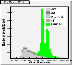
Qualitatively, the overall size of the signal is set by the fermion-resonance coupling $\sigma\propto g_{ffV}^{2}$ and the mass scale of the new resonances ($M_{W_{1}}\sim 1/l_{1}$), while the relative height of the peaks is determined by the relative strengths of the couplings $g_{W_{1}WZ},g_{W_{2}WZ}$ and the mass separation $M_{W_{2}}-M_{W_{1}}$, both of which depend (primarily) on the geometry parameters $o_{V},o_{A}$. Preliminary studies of the $o_{V},o_{A}$ and $l_{1}$ dependence of $g_{W_{1}WZ},g_{W_{2}WZ}$ are being carried out [93], however a more thorough analysis of the HTC parameter space remains to be done.

The large s-channel signals to $WZ$ look similar to signals of Low-Scale Technicolor (LSTC) [67, 68, 66]. However, in LSTC the interactions are carefully chosen to preserve an approximate techni-parity symmetry. With this symmetry only the vector resonance couples to longitudinal $W$ and $Z$ polarizations. In HTC, we are not free to tune the interactions. All interactions, including vector-axial mixing, are determined by the 5D parameters and boundary conditions. In the region of interest (viable with electroweak constraints) we find that techni-parity is not a good approximation for HTC, so both low-lying resonances couple to $W_{L},Z_{L}$. Since the resonance contribution to ${\rm pp}\rightarrow WZ$ is dominated by $W_{1,2}\rightarrow W^{\pm}_{L}Z_{L}$ , LSTC predicts only one peak in figure (2), while in HTC we see two.

Another interesting s-channel production mode is

$${\rm pp}\rightarrow W^{\pm}_{1,2}\rightarrow W^{\pm}\gamma\leavevmode\nobreak\ ,\leavevmode\nobreak\ W\rightarrow\ell\nu$$ (3)

Of the conventional three vector boson terms, the only permutation consistent with $U(1)_{em}$ gauge invariance is $g_{\gamma W_{1,2}W}(\partial_{[\mu}A_{\nu]}(W_{1,2[\mu}^{-}W^{+}_{\nu]})+h.c.),$ i.e. where the derivative acts on the photon field. A nonzero value for only one triboson coupling permutation is not possible in traditional, AdS-based Higgsless models. However, this final state as been considered recently [94] in the context of LSTC, exhibiting only one resonance.

This channel was also investigated in [92], and in figure (3) we plot the invariant $W+\gamma$ mass for the same sample HTC points used in figure (2).

Figure 3: Invariant mass for $W_{1,2}$ signal and background in the $W\gamma$ channel assuming $\mathcal{L}=10\ {\rm fb}^{-1}$. The HTC points are the same as in Figure (2). The dominant backgrounds are SM $W+\gamma$, and $W+{\rm jet}$ where the jet fakes a photon. The background is suppressed through hard cuts on $p_{T,\gamma},p_{T,W}$.

As in the $WZ$ case, the signals for both these HTC points are dramatic and could be seen within the first few ${\rm fb}^{{}_{{}^{-1}}}$. However, the difference between HTC parameters sets is more evident here than in the $WZ$ case. When $o_{V},o_{A}$ are such that the separation between the resonances is $\gtrsim 100\ {\rm GeV}$, as in the righthand plot, only the lightest resonance is visible, whereas in the $WZ$ case the second peak is still visible. The main reason for this is that the decay modes $W_{2}\rightarrow W_{1}Z,Z_{1}W$ are open, thus suppressing the branching ratio to $W\gamma$. Since the BR to $W\gamma$ is smaller than to $WZ$, only when the resonances are very degenerate, as in the lefthand example, are both resonances visible.

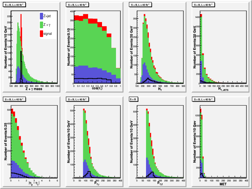
Finally, neutral resonances $Z_{1,2}$ can also be produced in the s-channel, but the most promising final state is into leptons rather than gauge bosons $WW$. Despite the smaller cross section, the cleaner dilepton channel may reveal both resonances within $\mathcal{L}\sim{\rm few\ }{\rm fb}^{-1}$ for the two points presented here.

5 VECTOR BOSON FUSION:

Although $s$-channel processes will be the most important in the early years of the LHC, alternative channels do exist and can expose different aspects of the resonance theory. One example process is vector boson fusion (VBF): ${\rm pp}\rightarrow W^{\pm}_{1,2}jj,Z_{1,2}jj$. For resonances decaying to a pair of gauge bosons, VBF directly probes $W_{L}W_{L}$ scattering and thus it is important to study regardless of the fermion-resonance coupling . One VBF channel, ${\rm pp}\rightarrow W^{\pm}_{1,2}jj\rightarrow W^{\pm}Zjj$, was studied in [92]. For the two HTC points, the existence of two nearby resonances could be seen as two edges in the transverse mass  $M_{T}$, though only with luminosity $\mathcal{L}\gtrsim O(100)\ {\rm fb}^{-1}$. VBF signals which require the $g_{W_{1,2}W\gamma}$ coupling, such as ${\rm pp}\rightarrow W^{\pm}\gamma jj$, may also be interesting.

6 CONCLUSIONS:

An effective lagrangian description of two new triplets of vector resonances would introduce ${\cal O}(100)$ new parameters. In this paper we perform a first step towards an economical parametrization of models of Dynamical EWSB: Holographic Technicolor (HTC). Although a departure from 5D modelling, HTC uses 5D techniques to parameterize a wide class of models in terms of 4 parameters: $l_{1},o_{V},o_{A},g_{ffV}$. After imposing current experimental constraints, we identified the relevant region in the HTC parameter space. We have chosen two sample HTC points and discussed the early discovery (${\cal L}\sim 10\ {\rm fb}^{-1}$) of two nearby resonances in the s-channel $pp\rightarrow W_{1,2}\rightarrow WZ,W\gamma$. The framework presented here can be extended to add new particles, e.g. techni-pions, techni-omegas and composite Higgs.

ACKNOWLEDGEMENTS:

We thank T. Appelquist, G. Azuelos, G. Brooijmans, K. Lane, S. Chivukula, N. Christensen, M. Perelstein and W. Skiba for helpful comments. The work of JH and AM is supported by DOE grant DE-FG02-92ER-40704 and VS is supported by DE-FG02-91ER40676.

blabla

Dilepton Final States

Part 6 Generic Searches for New Physics in the Dilepton Channel at the Large Hadron Collider

G. Landsberg

1 INTRODUCTION

This letter is devoted to searches for signals for new physics at the Large Hadron Collider (LHC) in the dilepton channel This channel has been historically fruitful for discoveries: $J/psi$ and $\Upsilon$ mesons, as well as the $Z$ boson were all discovered using dileptons. The LHC may not be an exception!

The advantages of the dilepton channels for searches for new physics are numerous:

• Easy triggering;

• Relatively low instrumental and standard model (Drell-Yan) backgrounds;

• Well known (NNLO) standard model (SM) cross section;

• Number of theoretical models that predicts relatively narrow resonances with non-vanishing decay branching fraction to dileptons; a typical example is a generic type of models with an extra $U(1)$ group, which leads to the existence of a $Z^{\prime}$ boson, often with non-zero couplings to dileptons.

2 THE MODEL

In the SM, the dilepton final state at hadron colliders is produced via the $s$ and $t$-channel exchange of virtual photons or $Z$ bosons. While the $s$ and $t$-channel diagrams interfere, their main contributions are well separated in the phase space of the dilepton system: high-$p_{T}$ dileptons are dominantly produced via the $s$-channel exchange, while the $t$-channel process mainly results in very forward leptons. While this doesn’t really matter for the generic formalism discussed below, we will focus on the high-$p_{T}$ dileptons in the $s$-channel, as the most promising signature for new physics at the LHC, with the exception of one case – $t$-channel exchange of a leptoquark (LQ) or a SUSY particle in the models with $R$-parity violation (RPV).

In the presence of additional diagrams contributing to the dilepton final state via exchange of new particles, the overall cross section for the dilepton production is given by the interference of the SM diagrams with the new ones coming from new physics. Consequently, it makes sense to parameterize the double-differential cross section, $d^{2}\sigma/dM_{ll}/d\cos\theta^{*}$, where $M_{ll}$ is the dilepton invariant mass and $\cos\theta^{*}$ is the cosine of the scattering angle in the dilepton c.o.m. frame, in the following form:

$$\frac{d^{2}\sigma}{dM_{ll}d\cos\theta^{*}}=\left(\frac{d^{2}\sigma}{dM_{ll}d\cos\theta^{*}}\right)_{\rm SM}+\left(\frac{d^{2}\sigma}{dM_{ll}d\cos\theta^{*}}\right)_{\rm int}+\left(\frac{d^{2}\sigma}{dM_{ll}d\cos\theta^{*}}\right)_{\rm NP}.$$ (1)

Here the first term describes the SM contribution, the second term corresponds to the interference between the SM and new physics contributions, and the third one describes direct contribution from new physics. In terms of matrix elements, the first three terms are proportional to the appropriate derivatives of $|{\cal M}_{\rm SM}|^{2}$, $|{\cal M}_{\rm SM}^{*}{\cal M}_{\rm NP}+{\cal M}_{\rm SM}{\cal M}_{\rm NP}^{*}|$, and $|{\cal M}_{\rm NP}|^{2}$, respectively.

Eq. (1) describes well general case of new physics due to, e.g., compositeness-like operator. However, in case new physics appears in a form of a narrow resonance, the corresponding matrix element has a Breit-Wigner pole, and therefore it makes sense to explicitly specify it. Moreover, in the case of relatively narrow resonance, the interference effect nearly cancels out when integrating over the width of the resonance, so it simply could be added to the above equation:

$$\frac{d^{2}\sigma}{dM_{ll}d\cos\theta^{*}} = \left(\frac{d^{2}\sigma}{dM_{ll}d\cos\theta^{*}}\right)_{\rm SM}+\left(\frac{d^{2}\sigma}{dM_{ll}d\cos\theta^{*}}\right)_{\rm int}+\left(\frac{d^{2}\sigma}{dM_{ll}d\cos\theta^{*}}\right)_{\rm NP}+$$ (2)

$${\rm BW}(M_{ll},M_{0},\Gamma_{0})\frac{d\Omega}{d\cos\theta^{*}},$$

where BW is the line-shape for a Breit-Wigner resonance with the mass $M_{0}$ and width $\Gamma_{0}$, and $\Omega$ is the angular distribution of its decay products. The remaining NP contribution described by the second two terms now does not include the resonance, which has been explicitly treated separately. In case of more than one resonance (e.g., Kaluza-Klein tower of resonances), additional terms similar to the last one can be added. However, since e focus our attention on early searches for new physics, chances are that only the lowest mass resonance is going to be visible.

Note that the advantage of using double-differential cross section for description of the process is that the two variables, $M_{ll}$ and $\cos\theta^{*}$ define the tree-level $2\to 2$ process completely. Thus, at leading order, they contain entire information about both the SM and new physics contributions, i.e. offer the most powerful separation between the NP signal and SM background possible in the entire phase space.

An additional advantage of using full double-differential cross section is that the “standard candle” – the $Z$ peak – is contained in the data. That allows in situ calibration of the search sample: in particular the limits on new physics cross section, or the measurement of its cross section can be expressed in terms of the $Z$ production cross section, which is well-known theoretically. Moreover, normalization to the $Z$-peak results in the reduced systematic error, as many important uncertainties, such as the uncertainty of the luminosity measurements, signal acceptance, and lepton identification efficiency would largely cancel out.

3 THE METHOD

The proposed method to look for generic deviations due to NP effects is based on the idea outlined in Ref. [95], generalized to a more complete case of non-resonant and resonant NP contributions.

The fist step is to generate templates corresponding to each of the four terms of Eq. (2) for a particular model. The simplest one would have a flat resonance decay angular distributions, i.e. $d\Omega/d\cos\theta^{*}=$const, and a particular non-resonant NP model, e.g., compositeness. These templates are result of parton-level Monte-Carlo (MC), followed by the detector simulation, which includes acceptance requirements as well as smearing of particle momenta. Once the templates are generated, one would fit experimental $d^{2}\sigma/dM_{ll}d\cos\theta^{*}$ spectrum (typically in a form of a 2-dimensional histogram) to the sum of four terms. The results of the fit can then be used to evaluate the relative weights of the SM-only and SM $+$ NP hypotheses and distinguish between various types of new physics. The MC templates also include next-to-leading order corrections in the form of non-zero transverse momentum of the dilepton system. Since the final state is colorless, the new particles contributing to the final state must be color-singlet as well. That implies that the only source of next-to-leading order corrections is initial-state radiation, which is expected to be the same for the Drell-Yan dilepton production and for contributions from new physics. Thus the $p_{T}$ spectrum of the dilepton system can be reliably modeled by using the well-known $p_{T}$ spectrum of Drell-Yan pairs.

Since for a heavy narrow resonance experimental mass resolution is typically worse than the internal width, $\Gamma$, after the detector effects the Breit-Wigner in Eq. (2) will be replaced with a Gaussian with the r.m.s. $\sigma$ determined by the experimental mass resolution. (In case the resonance is not sufficiently narrow, a convolution of the Breit-Wigner and a Gaussian should be used instead.)

We can further quantify effects of non-resonant new physics via a parameter $\eta$, which shows the relative strength of the NP contribution. For example, if the new physics has characteristics of compositeness with the scale $\Lambda$, a good choice for this parameter is $\eta=1/\Lambda^{2}$. Putting it all together, we obtain a modified Eq. (2):

$$\frac{d^{2}\sigma}{dM_{ll}d\cos\theta^{*}}=f_{0}(M_{ll},\cos\theta^{*})+\eta f_{1}(M_{ll},\cos\theta^{*})+\eta^{2}f_{2}(M_{ll},\cos\theta^{*})+N\times G(M_{0},\sigma)f_{3}(\cos\theta^{*}),$$ (3)

where $f_{0}$, $f_{1}$, $f_{2}$ and $f_{3}$ are the templates discussed above, $G(M_{0},\sigma)$ is the Gaussian, and $N$ is the normalization. An example of templates from Ref. [95] is shown in Fig. 1.

Figure 1: Examples of the templates for Drell-Yan production at the Tevatron: a) the SM ($f_{0}$); b) $f_{1}$ for models with large extra dimensions; c) $f_{2}$ for models with large extra dimensions. Here $\eta$ is related to the ultraviolet cutoff for the Kaluza-Klein graviton tower, $M_{S}$ as $\eta=1/M_{S}^{2}$. From Ref. [95].

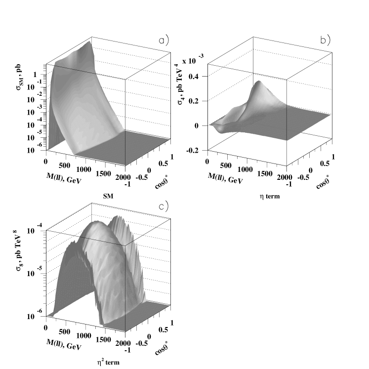
The fit of the double-differential distribution in data with the function described in Eq. (3) yields the values and the uncertainties on the two free parameters of the fit: $\eta$ and $N$. Depending on the values of these parameters, the following broad classes of new physics can be identified and possibly distinguished from one the other by doing steps outlined in the last column of the Table:

Table 1: Contributions of various types of new physics in the dilepton final state.

New physics model	$\eta$	$N$	Next steps
Standard Model	$=0$	$=0$	Look elsewhere
Compositeness	$\neq 0$	$=0$	Look at diphotons, dijets; correlate dielectrons and dimuons.
Large extra dimensions	$\neq 0$	$=0$	Look at diphotons, search for black holes and monojets.
LQ’s, RPV SUSY	$\neq 0$	$=0$	Look for pair-produced leptoquarks in the dilepton $+$ dijet
			channel; focus on a dedicated search for RPV SUSY.
$Z^{\prime}$	$=0$	$\neq 0$	Confirm absence in the $\gamma\gamma$ channel, determine couplings.
Randall-Sundrum model	$=0$	$\neq 0$	Confirm presence in the $\gamma\gamma$ channel, look for black holes.
Technirho/Tecniomega	$=0$	$\neq 0$	Confirm in the $W+$ dijet channel.
$Z_{KK}$	$\neq 0$	$\neq 0$	Correlate destructive interference with the peak height;
			look for the next excitation.

A simpler version of this method has been successfully used by the DØ experiment in searches for large extra dimensions [96, 97]. It is therefore expected that the above method would work well at the LHC.

4 CONCLUSIONS

A framework for generic searches for new physics in the dilepton channel at the LHC is discussed. This framework would allow to statistically distinguish between various models of new physics and to determine parameters (or set limits on their values) within a particular model.

ACKNOWLEDGEMENTS

I am grateful to my co-author on the original paper introducing this idea in the context of searches for large extra dimensions, Kingman Cheung. I would like to thank the Les Houches 2007 workshop organizers for an excellent and exciting venue, and the participants of the dilepton group for a number of stimulating discussions and suggestions. This work is partially supported by the U.S. Department of Energy under Grant No. DE-FG02-91ER40688 and by the National Science Foundation under the CAREER Award PHY-0239367.

Part 7 $Z^{\prime}$ Rapidity and Couplings to Quarks

T.M.P. Tait

1 INTRODUCTION

A massive neutral vector $Z^{\prime}$ decaying into a pair of leptons would be a fascinating discovery of physics beyond the Standard Model, one the LHC could hope to identify with a relatively small sample of data provided it couples to up- or down-type quarks and decays into charged leptons, $\ell^{+}\ell^{-}=e^{+}e^{-}$ or $\mu^{+}\mu^{-}$. After the initial excitement of discovery, it will be important to measure as many of the $Z^{\prime}$ couplings independently as possible, to unravel the underlying model from which it arose.

The primary initial observables will be the mass, given by the position of the excess in the lepton invariant mass distribution, and the cross section, given by the magnitude of the excess. Assuming the $Z^{\prime}$ has flavor universal couplings (motivated so that it does not introduce large FCNCs), the cross section can be parameterized at a hadron collider by [98],

$$\sigma(pp\rightarrow Z^{\prime}\rightarrow\ell^{+}\ell^{-}X) = c_{u}w_{u}+c_{d}w_{d}$$ (1)

where the $w_{u}$ and $w_{d}$ factors contain the parton distribution functions and higher order QCD corrections (exactly at NLO and to good approximation to NNLO) and thus contain only SM inputs, and $c_{u}$ and $c_{d}$ contain the $Z^{\prime}$-dependent quantities,

$$c_{u} = \left(g_{Q}^{2}+g_{u}^{2}\right)BR\left(Z^{\prime}\rightarrow\ell^{+}\ell^{-}\right)$$

$$c_{d} = \left(g_{Q}^{2}+g_{d}^{2}\right)BR\left(Z^{\prime}\rightarrow\ell^{+}\ell^{-}\right)$$ (2)

where $g_{Q}$, $g_{u}$, and $g_{d}$ are the $Z^{\prime}$ coupling to left-handed quarks (assumed equal by $SU(2)_{L}$ invariance), right-handed up-type quarks, and right-handed down-type quarks, and $BR(Z^{\prime}\rightarrow\ell^{+}\ell^{-})$ is the branching ratio into $\ell^{+}\ell^{-}$.

2 $c_{u}$ VERSUS $c_{d}$

A measurement of the cross section becomes, through, Eq. (1), a determination of a combination of couplings times the branching ratio into leptons. A single measurement constrains only a combination weighted by $w_{u}$ and $w_{d}$. As a first step toward separating out $c_{u}$ and $c_{d}$ individually, we consider the cross section differential in the rapidity distribution of the $Z^{\prime}$, $d\sigma/dy$. We expect that because there are more up than down quarks in the proton, that the contribution to forward $Z^{\prime}$ rapdities will depend more strongly on the coupling to up quarks than to down quarks. This can be captured by introducing $y$-dependent $w_{u,d}(y)$,

$$\frac{d\sigma}{dy_{Z^{\prime}}} = c_{u}w_{u}(y_{Z^{\prime}})+c_{d}w_{d}(y_{Z^{\prime}})$$ (3)

where the integral of $w_{u(d)}(y)$ over $y$ reproduces the original $w_{u(d)}$ in Eq. (1) for the inclusive $Z^{\prime}$ cross section.

To illustrate how this works, in Figure 1, we present the ratio of $w_{u}(y)/w_{d}(y)$ as a function of $y$ for a $Z^{\prime}$ of mass 2 TeV, computed at tree level. A more precise analysis would want to use higher order corrections, which are known to NNLO for this distribution [99], and are straight-forward to include. For this study which aims to examine a proof of principle, tree level is sufficient to estimate the utility of the measurement. (This quantity is equivalent to the ratio of cross sections $d\sigma/dy$ for two $Z^{\prime}$s of equal masses and couplings, one coupling only to $u$-quarks and the other coupling only to $d$-quarks). We see that at high rapidities $w_{u}(y)\gg w_{d}(y)$, and the sensitivity to the up-type quark couplings is enhanced.

Figure 1: Left: The ratio of $w_{u}(y)/w_{d}(y)$ as a function of $y$. Right: The uncertainties on the combination of $c_{u}$ and $c_{d}$ obtained from inclusive (red) and differential (blue) $Z^{\prime}$ cross section measurements, for the $Z^{\prime}$ considered in the text.

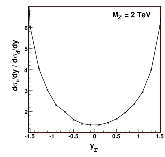
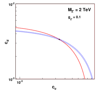
As an example to illustrate how this could work, we consider an example $Z^{\prime}$ with $M_{Z^{\prime}}=2$ TeV, $g_{Z^{\prime}}=0.1$, for which all quarks and leptons have the same charge (taken to be unity). This $Z^{\prime}$ has $c_{u}=c_{d}\simeq 3.2\times 10^{-3}$ and is compatible with LEP-II data. We imagine two measurements - one of the inclusive $Z^{\prime}\rightarrow e^{+}e^{-},\mu^{+}\mu^{-}$ and another with a cut of $|y_{Z^{\prime}}|>1$, selecting only $Z^{\prime}$s in the forward region. No detector effects or efficiencies are included. We apply statistical errors assuming $100\leavevmode\nobreak\ {\rm fb}^{-1}$ of collected data. These turn out to be on the order of $1\%$ ($3\%$) for the inclusive (cut) $Z^{\prime}$ cross sections we consider, and thus are probably similar in magnitude to the the residual theoretical error in an NNLO calculation, and coming from the PDFs.

We unfold the $1\sigma$ uncertainties in the combination of $c_{u}$ and $c_{d}$ for both measurements and plot the results in Figure 1. Also shown on the plot is the correct value of $c_{u}$ and $c_{d}$ for the example $Z^{\prime}$. The plot illustrates that adding the measurement of the cut $Z^{\prime}$ cross section does help break the degeneracy in $c_{u}$ and $c_{d}$ which is left after measuring the inclusive cross section.

3 CONCLUSIONS

We examine the possibility that one can use the $Z^{\prime}$ rapidity distribution to help disentangle the coupling of the $Z^{\prime}$ to up- and down-type quarks. The result is encouraging, and would motivate further investigation, including realistic detector simulations, a better treatment of uncertainties, and a more sophisticated analysis such as comparison with the full $Z^{\prime}$ rapidity distribution (and not just a cut rate measurement).

Between the time this study was performed at Les Houches 07 and the writing of this report, a more comprehensive theoretical treatment of $Z^{\prime}$ observables at the LHC has appeared [100], including discussion of this (and other) observables. The results of that study seem to continue to suggest that the $Z^{\prime}$ rapidity distribution is a useful quantity to unravel the $Z^{\prime}$ couplings to quarks.

ACKNOWLEDGEMENTS

Research is supported at Argonne National Lab by the US Department of Energy under contract DE-AC02-06CH11357. It is a pleasure to acknowledge the organizers of Les Houches for a stimulating physics environment, and the LAPTH theory group for their hospitality while some of the work herein was completed.

Part 8 A search for top partners at the LHC using same-sign dilepton final states

T. Bose, R. Contino, M. Narain and G. Servant

1 INTRODUCTION

The most notorious example of symmetry protection for the light Higgs is Supersymmetry: according to its paradigm, the radiative correction of each SM field to the Higgs mass is fine tuned against that of a superpartner of opposite statistics. The top quark contribution, in particular, is balanced by the contribution of its scalar partners, the stops. Another kind of symmetry protection, however, could be at work: the light Higgs could be the pseudo-Goldstone boson of a spontaneously broken global symmetry [101, 102, 103]. In this case the radiative correction of the top quark to the Higgs mass is balanced by the contribution of new partners of the same spin. The naturalness criterium suggests that these new heavy fermions should have masses below, or not much heavier than, 1 TeV. The production and detection of these top partners at the LHC was studied in [104] focussing on final states with two same-sign leptons. This note reports those findings and complements them with a preliminary analysis using the CMS Fast Simulation [105].

Particularly motivated is the possibility that the spontaneous breaking of the global symmetry and the new states originate from a strongly-coupled dynamics. This would allow for a complete resolution of the Hierarchy Problem without the need of fundamental scalar fields, and would make it possible to generate a large enough quartic coupling for the Higgs via radiative effects.

The LEP precision data are crucial in guiding our theoretical investigation, as they seem to be compatible only with a specific kind of strong dynamics: the new sector must possess a custodial symmetry $G_{C}=$SU(2)_C to avoid large tree-level corrections to the $\rho$ parameter [106]. This in turn implies an unbroken SU(2)${}_{L}\times$SU(2)${}_{R}\times$U(1)_X invariance of the strong dynamics before EWSB, meaning that its resonances, in particular the heavy partners of the top quark, will fill multiplets of such symmetry. It has been recently pointed out [107] that the LEP constraint on the $Z\bar{b}_{L}b_{L}$ coupling is more easily satisfied if the custodial symmetry of the strong sector includes a $LR$ parity, $G_{C}=$SU(2)${}_{C}\times P_{LR}$, and $b_{L}$ couples linearly to a composite fermionic operator transforming as a $(\mathbf{2},\mathbf{2})_{2/3}$ under SU(2)${}_{L}\times$SU(2)${}_{R}\times$U(1)_X (hypercharge being defined as $Y=T^{3}_{R}+X$). In this case, the heavy partners of $(t_{L},b_{L})$ can themselves fill a $(\mathbf{2},\mathbf{2})_{2/3}$ representation. The latter consists of two SU(2)_L doublets: the first, $(T,B)$, has the quantum numbers of $(t_{L},b_{L})$; the second – its “custodian” – is made of one fermion with exotic electric charge $Q_{e}=+5/3$, $T_{5/3}$, and one with charge $Q_{e}=+2/3$, $T_{2/3}$. Since the Higgs transforms like a $(\mathbf{2},\mathbf{2})_{0}$, the partners of $t_{R}$, if any, will form a $(\mathbf{1},\mathbf{1})_{2/3}$ or a $[(\mathbf{1},\mathbf{3})\oplus(\mathbf{3},\mathbf{1})]_{2/3}$ of SU(2)${}_{L}\times$SU(2)${}_{R}\times$U(1)_X [107].

As discussed in more details in Ref. [104], these heavy partners couple strongly to the third generation SM quarks plus one longitudinal $W$, $Z$ gauge boson or the Higgs. As in [104], we focus on the pair production of the $B$ and of its custodial partner $T_{5/3}$. Once pair produced, both the heavy bottom $B$ and the exotic $T_{5/3}$ decay exclusively to $W^{+}W^{+}W^{-}W^{-}b\bar{b}$, although with different spatial configurations as dictated by their different electric charges, see Fig. 1. In the case of the $T_{5/3}$ the same-sign $W$’s come from the decay of the same heavy fermion, while in the case of the heavy bottom they come from different $B$’s. Selecting events with two same-sign leptons thus allows one to fully reconstruct the hadronically-decaying $T_{5/3}$. Even though a full reconstruction of the $B$ is not possible, it was found in [104] that the same-sign dilepton channel is probably the most promising one for its discovery (see [108, 109] for other recent studies of pair-production of $B$-type quarks).

In this work, we report some of the results derived in Ref. [104] and we improve on them by adding the CMS Fast Simulation [105] to the analysis. Section 2 presents our Monte Carlo simulations. In Section 3, we discuss our cuts and derive the discovery potential, while in Section 4 we reconstruct the $W$ and $t$ candidates and pair them to reconstruct the $T_{5/3}$ invariant mass.

Figure 1: Pair production of $T_{5/3}$ and $B$ to same-sign dilepton final states.

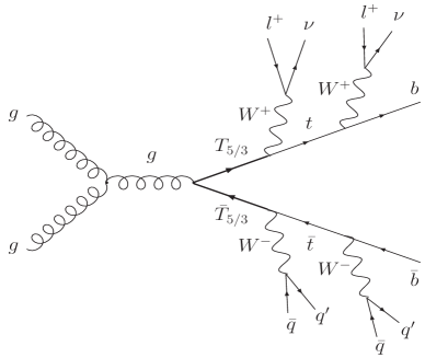
2 FAST SIMULATION AND EVENT SELECTION

We focus on the pair production at the LHC of $B$ and $T_{5/3}$ to two same-sign leptons :

$$gg,\,q\bar{q}\to B\bar{B},\,T_{5/3}\bar{T}_{5/3}\to t\overline{t}W^{+}W^{-}\to l^{\pm}\nu\,l^{\pm}\nu\,b\bar{b}\,q\bar{q}^{\prime}q\bar{q}^{\prime}\,.$$ (1)

The physical, observed final state is of the form

$$pp\to l^{\pm}l^{\pm}+n\;jets\,+\not\!\!E_{T}\,,\qquad\quad l=e,\mu\,,$$ (2)

where the number of jets depends on the adopted jet algorithm and on its parameters. We take $M=500$ GeV for the mass of the heavy fermions (we refer the reader to  [104] for the related study of the $M=1$ TeV case) and set the coupling to $tW$ to be $\lambda_{T_{5/3}}=\lambda_{B}=3$. Such large values of the couplings are naturally expected if the heavy fermions are bound states of a strongly coupled sector, and $t_{R}$ is mainly composite.

The most important SM backgrounds to the process of eq.(2) are $t\bar{t}W+jets$, $t\bar{t}WW+jets$ (including the $t\bar{t}h+jets$ resonant contribution for $m_{h}\geq 2m_{W}$), $WWW+jets$ (including the $Wh+jets$ resonant contribution for $m_{h}\geq 2m_{W}$), $W^{\pm}W^{\pm}+jets$ and $Wl^{+}l^{-}+jets$ (including the $WZ+jets$ contribution) where one lepton is missed. To be conservative and consider the case in which the background is largest, we have set the Higgs mass to $m_{h}=180\,\text{GeV}$. This greatly enhances the $t\bar{t}WW$ and $WWW$ backgrounds. The production cross sections for the signal and for the various backgrounds are reported in Table 1. No K-factors have been included, since those for the backgrounds are not all available (the K-factor for the signal is $\simeq 1.8$ for $M=500$ GeV [110]).

	$\sigma$ [fb]	$\sigma\times BR(l^{\pm}l^{\pm})$ [fb]
$T_{5/3}\overline{T}_{5/3}/B{\overline{B}}+jets$  $(M=500$ GeV)	$2.5\times 10^{3}$	104
$T_{5/3}\overline{T}_{5/3}/B{\overline{B}}+jets$  $(M=1$ TeV)	37	1.6
$t{\overline{t}}W^{+}W^{-}+jets$  ($\supset t\bar{t}h+jets$)	121	5.1
$t{\overline{t}}W^{\pm}+jets$	595	18.4
$W^{+}W^{-}W^{\pm}+jets$ ($\supset hW^{\pm}+jets$)	603	18.7
$W^{\pm}W^{\pm}+jets$	340	15.5

Table 1: Signal and background cross sections at leading order (left column). The right column reports the cross section times the branching ratio to two same-sign leptons final states ($e$ or $\mu$).

Given its complexity, we were not able to fully simulate the $Wl^{+}l^{-}+jets$ background, and for that reason we have not included it in our analysis. However, we estimated that after the main cuts presented below, the $Wl^{+}l^{-}+jets$ background is expected to be smaller than $\sim 30\%$ of the sum of the other backgrounds [104]. Even though this is not entirely negligible, the error due to its exclusion is within the uncertainty of our leading-order analysis. Moreover, the $Wl^{+}l^{-}+jets$ cross section is expected to be strongly suppressed after requiring the reconstruction of one $W$ and one top as done in the last section.

Another potential source of background are $t\bar{t}+jets$ events where the charge of one of the two leptons from the top decays is misidentified. Given the large $t\bar{t}+jets$ cross section, even a charge misidentification probability $\varepsilon_{mis}\sim\text{a few}\times 10^{-3}$ would result into a same-sign dilepton background of the same order of $t\bar{t}W+jets$.   The hardest lepton in the $t\bar{t}+jets$ events has a $p_{T}$ distribution peaked at values smaller than $100\,\text{GeV}$ (the second hardest lepton has instead a significantly softer $p_{T}$ distribution). From the latest ATLAS and CMS TDRs, probabilities as low as $\sim 10^{-4}$ seem to be realistic in the case of 100 GeV muons, while slightly larger values are expected for electrons [8, 111]. In such case the $t\bar{t}+jets$ background would be safely negligible. In the absence of a realistic estimate of $\varepsilon_{mis}$ as a function of the lepton’s $p_{T}$ and pseudo-rapidity, we decided not to include the $t\bar{t}+jets$ background events in our analysis. It is however clear that a specific and accurate estimate of this background is required to validate our results.

In these proceedings, we review part of the findings obtained with the simulation and analysis of Ref. [104], that we will refer to as generic analysis, and compare with the results obtained by adding the CMS Fast simulation of the detector. Both the signal and the SM background events were generated at the partonic level with MadGraph/MadEvent [35, 76, 112], .

In the generic analysis, we have used Pythia [75] for showering and to include the initial and final-state radiation. Hadronization and underlying event have been switched off for simplicity. Jets have been reconstructed using the GetJet [113] cone algorithm with $E_{T}^{min}=30\,\text{GeV}$ and a cone size $\Delta R=0.4$. The parton-jet matching has been performed following the MLM prescription [114, 115]. No detector effects were taken into account, except for a simple gaussian smearing on the jets. Both the jet energy and momentum absolute value were smeared by $\Delta E/E=100\%/\sqrt{E/\text{GeV}}$, and the jet momentum direction using an angle resolution $\Delta\phi=0.05$ radians and $\Delta\eta=0.04$.

On the other hand, in the CMS Fast Simulation analysis [105], the samples are first processed via PYTHIA for showering, to include initial and final-state radiation and to fragment and hadronize quarks and gluons. In addition, the underlying event is switched on. A jet-matching algorithm, following the MLM prescription [116] is employed to ensure that there is no double counting due to the parton showering in PYTHIA. These samples are then processed via a dedicated fast simulation processor (FAMOS) of the CMS detector and the event reconstruction software. Jets with cone size $\Delta R=0.5$ are reconstructed with the iterative cone algorithm. Generic jet energy corrections are applied to the cone jets. The jet resolution used in the CMS Fast Simulation is $\Delta E_{T}/E_{T}=1.25/\sqrt{E_{T}/\text{GeV}}\oplus 5.6/{E_{T}/\text{GeV}}\oplus 0.033$ [8]. This jet energy resolution will be the main source of different results with the generic analysis.

A first important information on the kinematics of signal and background events comes from the number of reconstructed jets. Fig. 2 compares the distributions for the number of jets in both analysis. The background and signal values are peaked at 2 and 5 (3 and 6) respectively in the generic (CMS Fast Simulation) analysis [105]. By signal here we mean either $T_{5/3}\bar{T}_{5/3}$ or $B\bar{B}$ events. The CMS Fast Simulation leads to a slightly larger number of reconstruted jets above $p_{T}>$ 30 GeV due to a combination of the underlying event settings, jet reconstruction algorithm, and energy corrections used.

Figure 2: Fractions of signal and background events with a given number of jets for $E^{min}_{T}=30\,\text{GeV}$. Left plot is from Ref. [104] (using the GetJet cone algorithm with $\Delta R=0.4$) and right plot is from the CMS Fast Simulation (using iterative cone algorithm with $\Delta R=0.5$).

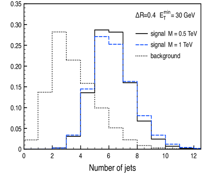
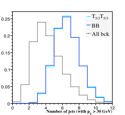
The total background distribution is peaked at smaller values. This is mainly due to the low jet multiplicity in the $WWW+jets$ and $W^{\pm}W^{\pm}+jets$ backgrounds. In the case of the signal, the hard scattering process produces $6$ quarks, after the decay of the top and of the $W$. It turns out that for $M=500\,\text{GeV}$ the 5-jet bin is mostly populated by events where the 6th jet is lost because it is too soft (i.e. it does not meet the minimum transverse energy requirement, $E_{T}\geq 30\,\text{GeV}$).

3 DISCOVERY POTENTIAL

In this section, we focus on the discovery of the top partners, proposing a simple strategy that does not rely on any sophisticated reconstruction, nor does it require $b$-tagging.

Figure 3: $p_{T}$ distributions of the first and fifth hardest jets (left) and of the first and second hardest leptons (right) before any cut (from the generic simulation).

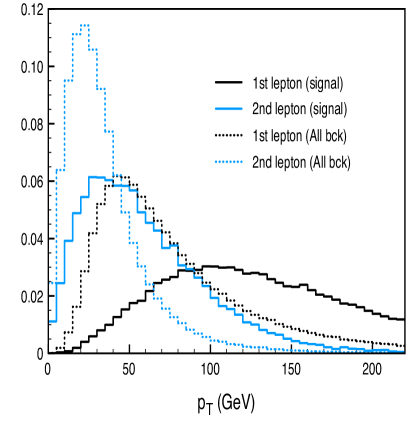
To isolate the signal, the following cuts are applied (both for the generic and the CMS Fast simulations):

$$\text{\text@underline{leptons}}:\begin{cases}p_{T}(\text{1st})\geq 50\;\text{GeV}\\ p_{T}(\text{2nd})\geq 25\;\text{GeV}\\ |\eta_{l}|\leq 2.4\,,\ \ \Delta R_{lj}\geq 0.4\end{cases}\quad\text{\text@underline{jets}}:\begin{cases}p_{T}(\text{1st})\geq 100\;\text{GeV}\\ p_{T}(\text{2nd})\geq 80\;\text{GeV}\\ n_{jet}\geq 5,\ \ |\eta_{j}|\leq 5\end{cases}\quad\not\!\!E_{T}\geq 20\;\text{GeV}\,,$$ (3)

where 1st and 2nd refer respectively to the first and second hardest jet or lepton (electron or muon). These cuts were motivated by the $p_{T}$ distributions shown in Fig. 3. The relative efficiencies are reported in Table 2.

	signal	$t\bar{t}W$	$t\bar{t}WW$	$WWW$	$W^{\pm}W^{\pm}$
	($M=500$ GeV)
Efficiencies ($\varepsilon_{main}$)	0.42   (0.55)	0.074   (0.15)	0.12   (0.06)	0.008   (0.02)	0.01   (0.03)
$\sigma\,\text{[fb]}\times BR\times\varepsilon_{main}$	44.2   (57.2)	1.4   (2.80)	0.62   (0.30)	0.15   (0.37)	0.16   (0.48)

Table 2: Efficiencies of the main cuts of eq.(3) for the generic analysis. Here signal means either $T_{5/3}\bar{T}_{5/3}$ or $B\bar{B}$ events. Numbers in parenthesis refer to the CMS Fast Simulation. [105]

After the cuts, the signal is much larger than the background. A rough indication on the mass of the heavy fermions can be extracted from the distribution for the scalar sum of $p_{T}$ of all jets in the event ($H_{T}$), see Fig. 4. This is a quantity that is not much affected by a poor jet energy resolution, and as such it is particularly appropriate in the first LHC phase. Further evidence on the production of a pair of heavy fermions comes from the distributions of the total invariant mass, the invariant mass of the hardest $5$ jets, and transverse mass of the $(ll\nu\nu j)$ system. We refer the interested reader to Ref. [104] for the relative plots.

Figure 4: $H_{T}$ distribution (scalar sum of $p_{T}$ of all jets in the event). Comparison between the simulation of Ref. [104] (left) and the output of the CMS Fast Simulation for an integrated luminosity corresponding to 1 $\text{fb}^{-1}$ (right).

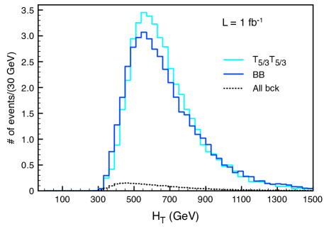
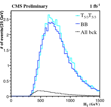
By counting the number of signal and background events that pass the main cuts of eq.(3), one can estimate the statistical significance of the signal over the background, as well as the minimum integrated luminosity required for a discovery. In the generic analysis, we defined the latter to be the integrated luminosity for which a goodness-of-fit test of the SM-only hypothesis with Poisson distribution gives a p-value = $2.85\times 10^{-7}$, (see for instance  [85]).  Results are reported in Table 3. The numbers in parenthesis are those from the CMS Fast simulation, were we used a different and more conservative estimate for the significance: $S/\sqrt{S+2B}$.

		${\cal S}$	${\cal B}$	$L_{disc}$
$M=500$ GeV	$T_{5/3}+B$	864  (1124)	23  (42)	$56$	$\,\text{pb}^{-1}$  (240 pb-1)
	$B$ only	424  (548)	23  (42)	$147$	$\,\text{pb}^{-1}$  (530 pb-1)

Table 3: Number of signal (${\cal S}$) and background (${\cal B}$) events that pass the main cuts of eq.(3) with $L=10\,\text{fb}^{-1}$ for $M=500\,\text{GeV}$. The last column reports the corresponding integrated luminosity needed for the discovery ($L_{disc}$), as computed in the generic analysis by means of a goodness-of-fit test with Poisson distribution and p-value = $2.85\times 10^{-7}$. Values in parenthesis are from the CMS Fast Simulation and in the last column $L_{disc}$ is computed using $S/\sqrt{S+2B}$ as an estimate of the significance.

In the most favorable case where both $T_{5/3}$ and $B$ partners exist and have mass $M=500\,\text{GeV}$, a discovery will need less than $\sim 250\,\text{pb}^{-1}$. Our estimates should be conservative, as we did not include any K-factor in our analysis, although it is known that next-to-leading order corrections enhance the signal cross section by $\sim 80\%$ for $M=500\,\text{GeV}$  [110]. Even a common K-factor $\kappa$ for both the signal and the background would imply a statistical significance larger by a factor $\sim\sqrt{\kappa}$, as well as a discovery luminosity smaller by the same factor.

4 $T_{5/3}$ MASS RECONSTRUCTION

More direct evidence for the production of a pair of $T_{5/3}$ or $B$ comes from reconstructing the hadronically decayed top quark and $W$ boson, as well as from the distribution of the invariant mass of their system. The mass reconstruction of $T_{5/3}$ crucially depends on the jet energy resolution when using the full detector simulation. We find that the width of the reconstructed top quark mass as obtained in the generic analysis is 12.5 GeV, while that obtained from the CMS Fast Simulation is about 19.5 GeV. This latter value more realistically reproduces the expected resolution of in the early phase of the LHC. It will improve as the flavor dependent jet energy corrections and use of high purity $b$-tagging for correct assignment of the $b$-jets are incorporated in the analysis.

We report here the results from the generic analysis using the energy resolution defined in Section 2, which is probably optimistic for the early LHC phase. We first select the events where two $W$’s can be simultaneously reconstructed, each $W$ candidate being formed by a pair of jets with invariant mass in the window $|M(jj)-m_{W}|\leq 20\,\text{GeV}$. To avoid wrong pairings and reduce the fake ones from the background, we impose the following cuts:

$$\Delta R_{jj}\leq 1.5\,,\quad|\vec{p}(W)|\geq 100\,\text{GeV} \text{on the first $W$ candidate}\,;$$ (4)

$$\Delta R_{jj}\leq 2.0\,,\quad|\vec{p}(W)|\geq 30\,\text{GeV} \text{on the second $W$ candidate}\,.$$ (5)

The $p_{T}$ cuts, in particular, have been optimized using the $p_{T}$ distributions of the $W$ and top from the signal events (see [104]). If more than one pair of $W$ candidates exists which satisfies the above cuts, we select that with the smallest $\chi^{2}=\Delta R_{jj}^{2}(\text{1st pair})+\Delta R_{jj}^{2}(\text{2nd pair})$. We then reconstruct the top by forming $Wj$ pairs, made of one $W$ and one of the remaining jets, with invariant mass in the window $|M(Wj)-m_{t}|\leq 25\,\text{GeV}$. If more than one top candidate exists, we select that with invariant mass closest to $m_{t}$. We discard events where no top can be reconstructed. The efficiencies of this reconstruction algorithm are reported in Table 4.

	signal	$t\bar{t}W$	$t\bar{t}WW$	$WWW$	$WW$
	($M=500$ GeV)
$\varepsilon_{2W}$	0.62	0.36	0.49	0.29	0.15
$\varepsilon_{top}$	0.65	0.56	0.64	0.35	0.35

Table 4: Efficiencies for the reconstruction of two $W$’s ($\varepsilon_{2W}$) and one top ($\varepsilon_{top}$) using the algorithm and the cuts described in the text for the case $M=500\,\text{GeV}$.

The distribution of the $Wt$ invariant mass is plotted in Fig. 5.

Figure 5: Invariant mass of the $Wt$ system for $M=500\,\text{GeV}$ with $L=10\,\text{fb}^{-1}$. The dotted curve refers to the case in which $b$-tagging is performed in the reconstruction. It assumes two $b$ tags, though no $b$-tagging efficiency has been included.

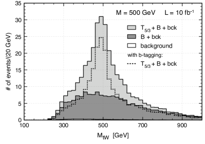
As expected, in the scenario with $T_{5/3}$ partners there is a resonant peak centered at $M_{T_{5/3}}=500\,\text{GeV}$, while the distribution has a non-resonant, continuous shape if only $Q_{e}=-1/3$ heavy fermions exist. The dotted curve refers to the case in which $b$-tagging is performed in the reconstruction algorithm. More in detail, we have selected events with two $b$ tags and we have reconstructed the top from $Wb$ pairs, excluding at the same time the $b$ jets when selecting the $W$ jet pair candidates. No $b$-tagging efficiency has been included, in order not to commit to any specific value (hence, for a $b$-tagging efficiency $\epsilon_{b}$ the final distribution will be rescaled by a factor $\epsilon_{b}^{2}$).

5 CONCLUSIONS

Our results show that the analysis of final states with two same-sign leptons at the LHC is an extremely promising method to discover the top partners $B$ and $T_{5/3}$. By requiring two same-sign leptons one avoids the large $t\bar{t}$ background and selects a particularly clean channel where evidence for the existence of the heavy fermions could come in the early phase of the LHC. If both $B$ and $T_{5/3}$ exist, a discovery will require only $\sim$ 60 – 250 pb^-1, depending on how the statistical significance is estimated. Even without $b$-tagging, and before reconstructing the hadronically decayed $W$ and top, one can have a first crucial indication on the value of the mass of the heavy fermions from the distributions of the total invariant mass, the invariant mass of the hardest $5$ jets or the $H_{T}$ distribution (scalar sum of jet $p_{T}$’s).

Ultimately, a crucial information to understand the origin and the role of the heavy fermions would come from the measurement of their decay width, which will in turn lead to a determination of their couplings $\lambda_{T_{5/3},B}$. A large value of $\lambda_{T_{5/3},B}$ will be strong circumstantial evidence for the compositeness of the heavy fermions. Extracting the decay width from the invariant mass distribution will be challenging, as one will have to cope with the issue of jet energy resolution. Most likely, a measurement will be possible only with large statistics and will require sophisticated $W$ and $t$ reconstruction techniques.

Given the strong theoretical motivations for a search of the heavy partners of the top, we think that our explorative study would also deserve to be followed by a more detailed investigation. Our results suggest that the same-sign dilepton channel might be one of the golden modes to discover the top partners $B$ and $T_{5/3}$, but only a complete analysis with a full simulation of the detector effects, an exact calculation of the $Wl^{+}l^{-}+jets$ and $t\bar{t}+jets$ backgrounds, and the use of fully realistic reconstruction techniques will eventually establish its ultimate potentialities.

ACKNOWLEDGEMENTS

We thank the organizers of the Les Houches workshop for their invitation to participate to a very fruitful meeting.

blabla

Single Lepton + X Final States

Part 9 Top Quark Pairs as a Model-Independent Discriminator of New Physics at the LHC

D.G.E. Walker

1 INTRODUCTION

A considerable number of experimentally viable extensions to the Standard Model (SM) have been proposed to describe electroweak symmetry breaking. A sample of popular scenarios include: the Minimal Supersymmetric Standard Model (MSSM) [117], models with new strong dynamics [118, 44, 119, 120, 121, 122, 49], composite Higgs models at the TeV scale [123], Little Higgs models [124, 125, 126], and models with extra dimensions at the electroweak scale [127, 128]. In addition, some string-inspired extensions [129, 130] can also lead to new signatures. In this review, we describe a scheme to sort out the particle content in a model independent fashion.

The LHC will be a “top factory”: About 80 million $t\bar{t}$ events will be produced via QCD production for integrated luminosity of 100 fb^-1. With such a large number of events (and knowing natural models have a preferential coupling to top quarks), it seems worthwhile to study top pairs. If the new physics contributes to $t\bar{t}$ production as an $s$-channel resonance, we want to identify the signal as a bump [131] on the smoothly falling $t\bar{t}$ invariant mass distribution. We want to then reconstruct the $t\bar{t}$ c.m. frame so the integer spin of the resonance can be determined from the polar angular distribution of the top quark. Further, any asymmetry of this distribution could probe possible chiral couplings. In addition, any CP properties of the couplings could be elucidated with the help of CP-odd kinematical variables constructed from the final state particle momenta.

We look at only the $t\bar{t}$ semileptonic decay mode: $t\bar{t}$ $\to bj_{1}j_{2}\ \bar{b}\ell^{-}\bar{\nu}+\mathrm{c.c.}$ where $\ell=e$ or $\mu$. The purely hadronic decay mode not only suffers from a much larger QCD background, but also loses the identification of $t$ from $\bar{t}$. For the purely leptonic mode, with a small branching fraction of about $4/81$, one cannot reconstruct the $\bar{t}t$ invariant mass with two missing neutrinos. Thus, our signal will be an isolated charged lepton plus missing energy ($E\!\!\!\!/_{T}$), 2 $b$-jets plus 2 light jets. Note: The branching ratio of the semileptonic to the hadronic channel is 2/3.

In this article, we summarize the analysis of [132]. Since [132] appeared, many papers have been published which look at the effectiveness of using top quarks to probe new physics. A brief sample of papers is [133, 134, 135, 136, 137, 138, 139, 140, 141, 142]. Please note: [132] focused on early indications of new physics by restricting to only 10 fb^-1 of data. When necessary, for emphasis, we include the relevant analysis for 100 fb^-1. In all, the exposition of this review follows [132] closely.

2 EVENT RECONSTRUCTION

In order to search for new physics, we first have to reliably reconstruction $t\bar{t}$ semileptonic decays at high invariant mass on an event-by-event basis. $t\bar{t}$ semileptonic decays contain a neutrino in the final state – thereby complicating the reconstruction. The transverse momentum of the neutrino is identified with the observed $E\!\!\!\!/_{T}$. The neutrino longitudinal momentum is subject to a two-fold ambiguity from solving the kinematic quadratic equation.

We choose a reconstruction method useful for high invariant mass $t\bar{t}$ events [132]. Several top reconstruction methods have been used at the Tevatron [143, 144]. There, however, the top quarks are produced near threshold and the kinematics of the subsequent decay products are very complicated. High invariant mass $t\bar{t}$ events tremendously simplify the kinematics, especially by distinguishing the $b$ quark from the $\bar{b}$. Throughout this review, we use a $2\to 6$ partonic level monte-carlo simulation that incorporates full spin correlations from production through decay [145, 146]. [132] made a Pythia simulation, including gluon radiation and hadronization, that confirmed the results presented here.

To ensure only high invariant mass $t\bar{t}$ events, we impose a cluster transverse mass cut on the $t\bar{t}$ system

$$M_{T}=\sqrt{(p_{b}+p_{\bar{b}}+p_{j_{1}}+p_{j_{2}}+p_{\ell})^{2}+E\!\!\!\!/_{T}^{2}}+E\!\!\!\!/_{T}>600\ {\rm GeV}.$$

Following ATLAS and CMS, we adopt the following kinematical cuts:

$$E_{T}^{j}>20\,\,\,\mathrm{GeV} |\eta_{j}|<2.5$$

$$p_{T}^{\ell}>20\,\,\,\mathrm{GeV} |\eta_{\ell}|<2.5.$$

In addition, we require a lepton-jet and jet-jet isolation cut and a $E\!\!\!\!/_{T}$ cut of

$$\Delta R>0.4 E\!\!\!\!/_{T}>20\,\,\,\mathrm{GeV}.$$

The hadronic energy is smeared according to a Gaussian error given by $\Delta E_{j}/E_{j}=0.5/\sqrt{E_{j}/\textrm{GeV}}\oplus 0.03$. Additionally, the lepton momentum is smeared by $\Delta p_{T}^{\ell}/p_{T}^{\ell}=0.36(p_{T}^{\ell}/\textrm{TeV})\oplus 0.013/\sqrt{\sin\theta}$. Here $\theta$ is the polar angle of the lepton with respect to the beam direction in the lab frame.

Figure 1: The $W$ and top mass reconstructions from our reconstruction scheme. Step I (Step II) is solid (dashed), respectively.

We choose a reconstruction scheme that takes $M_{W}$ and $m_{t}$ as inputs for their on-shell production and decays. We break the scheme into the following steps:

Step I: Demand $m_{l\nu}^{2}=M_{W}^{2}$. The longitudinal momentum of the neutrino is formally expressed as

$$p_{\nu L}=\frac{1}{2\,p_{eT}^{2}}\left({A\,p_{eL}\pm E_{e}\sqrt{A^{2}-4\,{p}^{\,2}_{eT}E\!\!\!\!/_{T}^{2}}}\right),$$

where $A=M_{W}^{2}+2\,\vec{p}_{eT}\cdot\,\vec{E\!\!\!\!/_{T}}$. If $A^{2}-4\,{p}^{\,2}_{eT}\,E\!\!\!\!/_{T}^{\,2}\geq 0$, the value of $p_{\nu L}$ that best yields the known top mass via $m_{l\nu b}^{2}=m_{t}^{2}$ is selected. This ideal situation may not always hold when taking into account the detector resolutions. For cases with no real solutions, we then proceed to the next step.

Step II: To better recover the correct kinematics, we instead first reconstruct the top quark directly by demanding $m_{l\nu b}^{2}=m_{t}^{2}$. The longitudinal momentum of the neutrino is expressed as

$$p_{\nu L} = {A^{\prime}\,p_{blL}}/2(E_{bl}^{2}-p_{blL}^{2})\ \pm\frac{1}{2(E_{bl}^{2}-p_{blL}^{2})}$$

$$\times ({{p_{blL}^{2}A^{{}^{\prime}\,2}+(E_{bl}^{2}-p_{blL}^{2})\,(A^{{}^{\prime}\,2}-4E_{bl}^{2}E\!\!\!\!/_{T}^{2})}})^{1/2},$$

where $A^{\prime}=m_{t}^{2}-M_{bl}^{2}+2\,\vec{p}_{blT}\cdot\,\vec{E\!\!\!\!/_{T}}$. The two-fold ambiguity is broken by choosing the value that best reconstructs $M_{W}^{2}=m_{l\nu}^{2}$. A plot of the top and $W$ mass distributions is shown in Fig. 1. The solid histogram is from the procedure Step I, and the dashed histogram from Step II. With these two steps, there could still be some events that do not lead to a real solution. Because we want accurate reconstruction of $t\bar{t}$ at high invariant mass, we thus discard them in our event collection. The discard rate is about 16%.

3 BACKGROUNDS

The major backgrounds to our $t\bar{t}$ events include the processes $W+$ jets, $Z+$ jets, $WW$, $WZ$ and $ZZ$. Both the ATLAS and CMS Technical Design Reports [37, 147] performed detailed studies of the selection efficiencies for these background processes in comparison to a reconstructed $t\bar{t}$ semileptonic signal. The ATLAS (CMS) group found for an integrated luminosity of $10$ fb^-1 ($1$ fb^-1) a signal to background ratio of $S/B=65$ ($S/B=26$). This ratio has been obtained using the kinematical cuts listed in the previous section. Because of the expected high $S/B$ ratio, our analysis is concentrated solely on the events without including the small background contamination. Our analysis does not include misidentification of faked leptons from jets in $t\bar{t}$ total hadronic decays.

Although the $t$ ($\bar{t}$) is primarily identified by the charged lepton, $\ell^{+}$ ($\ell^{-}$), a concern is the matching of the b-jet associated with this top quark decay. Both ATLAS and CMS studies [37, 147] show a combination of kinematic fits, designed to properly reconstruct the $W$ boson and the hadronically decaying top significantly reduces misidentification. The cut on $M_{T}$ helps significantly in this regard.

4 SEARCHING FOR NEW PHYSICS

Figure 2: Reconstructed $t\bar{t}$ invariant mass distributions. The plot features a 1 TeV resonance with a total width of 2% (solid), 5% (dashed), and 20% (dotted) of the resonance’s mass.

We want to search for new resonances that couple to $t\bar{t}$ in a model independent manner. We consider $t\bar{t}$ production via

$$gg\to\,\,\phi\to t\bar{t},\quad q\bar{q}\to\,\,V\to t\bar{t},\quad q\bar{q},\ gg\to\,\,\tilde{h}\to t\bar{t},$$

where $\phi$, $V$ and $\tilde{h}$ are the spin-0, spin-1, and spin-2 resonances. We characterize the effects on the invariant mass spectrum with three parameters: mass, total width, and the signal cross section normalization ($\omega^{2}$). The normalization $\omega=1$ defines our benchmark for the spin 0, 1 and 2 resonances. They correspond to the SM-like Higgs boson, a $Z^{\prime}$ with electroweak coupling strength and left (L) or right (R) chiral couplings to SM fermions, and the Randall-Sundrum graviton $\tilde{h}$ with the couplings scaled as $\Lambda^{-1}$ for $\tilde{h}q\bar{q}$, and $(\Lambda\ln(M^{*}_{pl}/\Lambda))^{-1}$ for $\tilde{h}gg$, respectively. Numerically, we take $\Lambda=2$ TeV.

Figure 3: Normalization factor versus the resonance mass for the scalar (dashed) with a width-mass ratio of $20\%$, vector (dot-dashed) with 5%, and graviton (solid) 2%, respectively. The region above each curve represents values of $\omega$ that give 5$\sigma$ or greater statistical significance with 10 fb^-1 (left panel) and 100 fb^-1 (right panel) integrated luminosity.

In Fig. 2 we show the reconstructed $t\bar{t}$ invariant mass distribution for our reconstruction scheme. The SM $t\bar{t}$ total cross section is theoretically known beyond the leading order in QCD [150, 151, 152]. We thus expect to have a good control of this distribution even at high invariant masses. As for new physics, we include the contribution of a 1 TeV vector resonance for illustration, for $\omega_{\mathrm{v}}=1$, with total widths specified in the caption of Fig 2.

We maximize the signal observability by isolating the resonance within an invariant mass window of $\pm 100$ GeV, $\pm 30$ GeV and $\pm 25$ GeV for the scalar, vector and graviton resonance, respectively. Given a resonance mass and total width, we can quantify how large $\omega$ needs to be for a $5\sigma$ discovery. With the number of events for a signal (S) and background (B), we require $S/\sqrt{B+S}>5$. This translates to a bound $\omega^{2}>(25+5\sqrt{25+4B})/2S_{1}$ where $S_{1}$ is the benchmark signal rate for $\omega=1$. This is illustrated by Fig. 3 versus the mass for a scalar, vector and graviton resonance for total widths of 20%, 5%, and 2% of its mass, respectively, for an integrated luminosity of 10 fb^-1 (Fig. 3, left panel) and 100 fb^-1 (Fig 3, right panel).

It is of critical importance to reconstruct the c.m. frame of the resonant particle, where the fundamental properties of the particle can be best studied. In Fig. 4, we show the top quark angular distribution, $\cos\theta^{*}$, with $\theta^{*}$ defined as the angle in the $t\bar{t}$ c.m. frame between the top-quark momentum and the incident quark momentum, with the latter determined by the longitudinal boost direction of the c.m. system. Although events in the forward and backward regions are suppressed due to the stringent kinematical cuts, we still see the impressive features of the $d$-function distributions in Fig. 4: a flat distribution for a scalar resonance (dashed), $d^{1}_{11}$ distribution for the left/right chiral couplings of a vector (dotted), and $d^{2}_{1\pm 1}$ from $q\bar{q}$ (solid) and $d^{2}_{2\pm 1}$ from $gg$ (dot-dashed) for a spin-2 resonance.

Figure 4: Polar angular distributions for the top quark in the c.m. frame, (a) Signal only by the for a scalar (dashed), a vector (dots), and a graviton from $q\bar{q}$ (solid) or from $gg$ (dot-dashed).

Figure 5: Polar angular distributions for the top quark in the c.m. frame. Number of events for the SM $t\bar{t}$ background (solid) with 1$\sigma$ statistical error bars, and the background plus a vector resonance (dashed) for (a) 10 fb^-1 and (b) 100 fb^-1

To illustrate the statistical sensitivity for observing the characteristic distributions, we show in Fig. 5 the expected SM $t\bar{t}$ events (solid) with 1$\sigma$ statistical error bars in each bin for a 10 fb^-1 and 100 fb^-1 integrated luminosity, along with a $5\sigma$ signal of a chirally coupled vector summed with the $t\bar{t}$ background in the resonant region (dashed). Due to the large event sample, the statistical significance is evident in the central and forward region. The forward-backward asymmetry in $\cos\theta^{*}$ can thus be constructed to probe the chiral couplings of the particle to the top quark. With the identification of the charged leptons, one may even form kinematical triple products to test the CP properties of the couplings [153, 154].

5 CONCLUSIONS

In summary, we reviewed the use for top quarks in discovering new physics in the form of integer-spin resonances. We showed the use of angular distributions of the top in the reconstructed CM frame to reveal the spin of the resonance, and the relative contribution from the initial states $q\bar{q}$ or $gg$. The forward-backward asymmetry and CP-odd variables can be constructed to further differentiate models. Because SM top quark physics is well predicted, high invariant mass top pair production may provide an early indicator for new physics beyond the Standard Model at the LHC.

ACKNOWLEDGEMENTS

The author thanks Vernon Barger and Tao Han for being part of a productive collaboration.

Part 10 Production of Kaluza–Klein excitations of gauge bosons at the LHC

A. Djouadi, G. Moreau and R.K. Singh

1 INTRODUCTION

If the extra–dimensional model suggested by Randall and Sundrum (RS) [128, 155] is to solve the gauge hierarchy problem of the Standard Model (SM), the masses of the first KK excitations of gauge bosons, $M_{\rm KK}$, must be in the vicinity of the TeV scale. Direct experimental searches for KK gluon excitations at the Tevatron lead to $M_{\rm KK}\gtrsim 800$ GeV [156, 157], while high–precision measurements impose stronger bounds as the exchanges of the KK excitations lead to unacceptably large contributions to the electroweak observables [158, 159, 160, 161, 162, 163]. Nevertheless, it was shown [16] that if the SM symmetry is enhanced to the left–right structure ${\rm SU(2)_{L}\!\times\!SU(2)_{R}\!\times\!U(1)_{\rm B-L}}$, with $B$ and $L$ the baryon and lepton numbers, electroweak precision data can be fitted while keeping the KK masses down to the acceptable value of $M_{\rm KK}\simeq 3$ TeV.

In the RS model with SM fields in the bulk, one can generate through a simple geometrical mechanism the large mass hierarchies prevailing among SM fermions [164] by placing them differently along the extra dimension: their different wave functions overlap with the Higgs boson, which remains confined on the so–called TeV–brane for its mass to be protected, generate hierarchical patterns among the effective four–dimensional Yukawa couplings. In this case, the KK gauge bosons dominantly couple to heavy SM fermions as they are localized toward the TeV–brane (this typical feature can only be avoided in some particular situations [165]). In this case, the processes involving the third generation $b$ and $t$ quarks are those which are expected to be significantly affected by the presence of the new vector states.

In the extended gauge symmetry originally proposed in Ref. [16], a ${\rm U(1)_{\rm B-L}}$ group was included; other ${\rm U(1)_{X}}$ groups with different fermion charges can be considered [107, 166]. An important motivation would be that with specific charges of the new Abelian group and for specific fermion localizations, the three standard discrepancy between the forward–backward asymmetry $A_{FB}^{b}$ in $Z\to b\bar{b}$ decays measured at LEP and the SM prediction [167] is naturally resolved, while keeping all the other observables in agreement with data. There are also constraints on the $t,b$ couplings from flavour changing neutral current processes, but those can be satisfied for $M_{KK}$ values around the TeV scale [168, 169, 170, 171, 172, 173, 174, 175].

At the LHC, one can produce directly the KK excitations of the gluons and the electroweak gauge bosons with masses in the multi–TeV range [176, 149, 134, 142, 137]. In this note, we study the main production mechanism, the Drell–Yan channel $pp\to V_{\rm KK}=g^{(1)},$ $\gamma^{(1)},$ $Z^{(1)},$ $Z^{{}^{\prime}(1)}$, and perform a Monte Carlo simulation of the process $q\bar{q}\to t\bar{t}$. We base our analysis on the framework which resolves the $A_{FB}^{b}$ anomaly [166], but the results that we obtain can be easily generalized to other scenarios. Including only the dominant QCD backgrounds, we show that for a set of characteristic points of the parameter space, the exchange of KK gauge bosons can lead to visible deviations with respect to the SM production rates.

2 PHYSICAL FRAMEWORK

We consider the RS model in which SM fields propagate along the extra spatial dimension, like gravity, but the Higgs boson remains confined on the TeV–brane. In the RS scenario, the warped extra dimension is compactified over a $S^{1}/\mathbb{Z}_{2}$ orbifold. While the gravity scale on the Planck–brane is $M_{P}=2.44\times 10^{18}$ GeV, the effective scale on the TeV–brane, $M_{\star}=e^{-\pi kR_{c}}M_{P}$, is suppressed by a warp factor which depends on the curvature radius of the anti–de Sitter space $1/k$ and the compactification radius $R_{c}$. The product $kR_{c}\simeq 11$ leads to $M_{\star}\!=\!{\cal O}(1)$ TeV, thus addressing the gauge hierarchy problem. The values for the fermion masses are dictated by their wave function localization. In order to control these localizations, the five–dimensional fermion fields $\Psi_{i}$, with $i=1,2,3$ being the generation index, are usually coupled to distinct masses $m_{i}$ in the fundamental theory. If $m_{i}={\rm sign}(y)c_{i}k$, where $y$ parameterizes the fifth dimension and $c_{i}$ are dimensionless parameters, the fields decompose as $\Psi_{i}(x^{\mu},y)=\sum_{n=0}^{\infty}\psi_{i}^{(n)}(x^{\mu})f_{n}^{i}(y)$, where $n$ labels the tower of KK excitations and $f_{0}^{i}(y)=e^{(2-c_{i})k|y|}/N_{0}^{i}$ with $N_{0}^{i}$ being a normalization factor. Hence, as $c_{i}$ increases, the wave function $f_{0}^{i}(y)$ tends to approach the Planck–brane at $y=0$.

We consider the scenario ‘RSb’ developed in Ref. [166] where, in order to protect the electroweak observables against large deviations and, at the same time, resolve the anomaly in $A_{FB}^{b}$, the electroweak gauge symmetry is enhanced to ${\rm SU(2)_{L}\times SU(2)_{R}\times U(1)_{X}}$ with some specific fermion representations/charges under the group gauge. The usual symmetry of the SM is recovered after the breaking of both ${\rm SU(2)_{R}}$ and ${\rm U(1)_{X}}$ on the Planck–brane, with possibly a small breaking of the ${\rm SU(2)_{R}}$ group in the bulk. Note the appearance of a new $Z^{\prime}$ boson (but without a zero–mode) which is a superposition of the state $\widetilde{W}^{3}$ associated to the ${\rm SU(2)_{R}}$ group and $\widetilde{B}$ associated to the ${\rm U(1)_{X}}$ factor; the orthogonal state is the SM hypercharge $B$ boson. Solving the gauge hierarchy problem forces the masses of the first KK excitations of the SM gauge bosons, $M_{\rm KK}=M_{\gamma^{(1)}}=M_{g^{(1)}}\simeq M_{Z^{(1)}}\simeq M_{Z^{\prime(1)}}$, to be ${\cal O}$(TeV) and we will fix the common mass value to $M_{\rm KK}=3$ TeV in the present study.

The light SM fermions [leptons and first/second generation quarks] are characterized by $c_{\rm light}>0.5$, $c$ being the parameter which determines the fermion localization to cope with high–precision data. The large value of the top quark mass requires $c_{t_{R}}<0.5$ and $c_{Q^{3}_{L}}<0.5$, with $c_{Q^{3}_{L}}\!=\!c_{t_{L}}\!=\!c_{b_{L}}$ [as the states $b_{L}$ and $t_{L}$ belong to the same ${\rm SU(2)_{L}}$ multiplet] so that the top and bottom quarks have to be treated separately. In the framework of Ref. [166], the precision data in the $b$ sector, that is $A_{FB}^{b}$ and $R_{b}$, are correctly reproduced with $M_{\rm KK}=3$ TeV and e.g. $g_{Z^{\prime}}=0.3\sqrt{4\pi}$ for the coupling of the new $Z^{\prime}$ boson. Then, the best fit of $R_{b}$ and $A_{FB}^{b}(\sqrt{s})$ (which also lead to the correct range for the top and bottom quark masses) is obtained for $c_{Q^{3}_{L}}\simeq 0.36$ and $c_{b_{R}}\simeq 0.135$. One gets the values $Q(c_{b_{R}})\simeq 3.04$ and $Q^{\prime}(c_{b_{R}})\simeq 3.19$, where $Q(c)$ ($Q^{\prime}(c)$) is the ratio of the four–dimensional effective coupling between the $g^{(1)}/\gamma^{(1)}/Z^{(1)}$ ($Z^{\prime(1)}$) boson and the SM fermions, over the coupling of the gluon/photon/$Z$ (would be $Z^{\prime}$) boson zero–mode. A small $Q$ charge holds for the light fermions, $Q(c_{\rm light})\simeq-0.2$, as well as zero $Z^{\prime}$ charge, $Q^{\prime}(c_{\rm light})=0$. This means that the couplings of the KK excitations of the gluon, photon and $Z$ boson are an order of magnitude smaller to light fermions compared to the couplings to top and bottom quarks, while the KK excitations of the $Z^{\prime}$ boson do not couple to these light fermions at all.

From the previous discussion, one concludes that in the chosen scenario, the sum of the branching ratios BR$(V_{\rm KK}\to t\bar{t})$ and BR$(V_{\rm KK}\to b\bar{b})$, with $V_{\rm KK}=\gamma^{(1)}$, $Z^{(1)}$, $Z^{\prime(1)}$ and $g^{(1)}$, is close to unity which means that the KK excitations decay almost exclusively into the heavy $t,b$ quarks and that little room is left for decays into light quarks and leptons. In the case of $g^{(1)}$ for instance, one has BR$(g^{(1)}\to t\bar{t})=0.69$ and BR$(g^{(1)}\to b\bar{b})=30$. Because of the large couplings to fermions, the total decay widths of the KK excitations $V_{\rm KK}$ [which grow proportionally to the mass $M_{V_{\rm KK}}\raisebox{-3.69899pt}{\leavevmode\nobreak\ \shortstack{$>$ \\ [-0.07cm] $\sim$}}\leavevmode\nobreak\ 3$ TeV] are very large. For instance, the decay width of $g^{(1)}$ is of the order of a few hundred GeV and is between 10% and 20% of its mass; the KK state can be thus considered as a relatively narrow resonance.

3 PRODUCTION CROSS SECTIONS AT THE LHC

The most straightforward way to produce the KK excitations of the gauge bosons $V_{\rm KK}$ at the LHC is via the Drell–Yan process, $pp\to q\bar{q}\to V_{\rm KK}\to Q\bar{Q}\,,\,Q=t,b$ with $V_{\rm KK}$ subsequently decaying into top and bottom quarks. The relatively small couplings of the initial quarks $q\equiv u,d,s,c$ to $V_{\rm KK}$ lead to smaller production rates compared to, for instance, the production of $Z^{\prime}$ bosons from GUT’s. Since the KK gauge bosons have different couplings to left– and right–handed fermions, one expects the produced $t/b$ quarks to be polarized and to have a forward–backward asymmetry. Because $V_{\rm KK}$ have substantial total decay widths, the narrow width approximation in which the production and decay processes are factorized is not sufficient and one needs to consider the virtual exchange of $V_{\rm KK}$ in which the total width is included in a Breit–Wigner form, together with the exchange of the zero modes; the full interference should be taken into account. For $b\bar{b}$ production, the subprocesses are also initiated by bottom partons and one should also consider the channel in which $V_{\rm KK}$ are exchanged in the $t$–channel.

The signal $q\bar{q}\to V_{\rm KK}\to Q\bar{Q}$ and the main SM background $q\bar{q}\to Q\bar{Q}$ and $gg\to Q\bar{Q}$ [which gives a much more substantial contribution] have to be considered simultaneously. For the signal reaction, we have calculated the matrix element squared of the process $pp\to Q\bar{Q}$ with polarized final state quarks and incorporated the exchange [including the $t$–channel contributions] of all the SM gauge bosons as well as their KK excitations and those of the $Z^{\prime}$ boson; we use the CTEQ5M1 set of parton distributions with the factorization and a renormalization scales set to the invariant mass of the $Q\bar{Q}$ system, $\mu_{F}=\mu_{R}=m_{Q\bar{Q}}$.The significance ${\cal S}$ of the signal in the RS model can be then defined as ${\cal S}_{\cal L}=(\sigma^{\rm RS+SM}-\sigma^{\rm SM})/(\sigma^{\rm SM})^{1/2}\times{\cal L}^{1/2}$ with ${\cal L}$ the total LHC luminosity.

In order to enhance the signal, which is peaked at $m_{Q\bar{Q}}$ and to suppress the continuum background, one needs to select events near the KK resonance. We thus impose the cut $|m_{Q\bar{Q}}-M_{\rm KK}|\leq\Gamma_{V_{\rm KK}}$. To further reduce the backgrounds, we also impose the following cuts on the transverse momenta of the two final jets and their rapidity $p_{T}^{Q,\bar{Q}}\geq 200\,{\rm GeV}$ and $|\eta_{Q,\bar{Q}}|\leq 2$, as in the signal, the $p_{T}$ of the jets is peaked close to $\frac{1}{2}M_{V_{\rm KK}}$ and the production is central, while in the background, the jets are peaked in the forward and backward directions and the bulk of the cross section is for low $p_{T}$ jets. These cuts can certainly be optimized but in this preliminary and simple parton–level investigation, we will simply compare the signal and the main corresponding physical background to determine if, grossly, one can have a detectable signal. More efficient and realistic cuts and detection efficiencies will not be discussed.

The invariant mass distribution d$\sigma$/d$m_{t\bar{t}}$ of the process $pp\to t\bar{t}$ is shown in the left–hand side of Fig. 1 for the chosen scenario with $M_{\rm KK}=3$ TeV, including the cuts mentioned above. As can be seen, there is a substantial contribution of the KK excitations to the invariant mass distribution, in particular around the peak $m_{t\bar{t}}\sim 3$ TeV. At higher $m_{t\bar{t}}$, the KK contribution becomes small, while at lower $m_{t\bar{t}}$, it is significant even for $m_{t\bar{t}}\sim 2$ TeV; only for $m_{t\bar{t}}\raisebox{-3.69899pt}{\leavevmode\nobreak\ \shortstack{$<$ \\ [-0.07cm] $\sim$}}\leavevmode\nobreak\ 1$ TeV the KK contribution becomes negligible. Outside the KK mass peak, the RS effect is mostly due to the interference between the excited state and SM contributions; this interference is positive below and negative above the peak. The dominant contribution compared to the SM case is by far due to the exchange of the excitation of $g^{(1)}$ which has the largest (QCD versus EW) couplings to the initial state partons; the contributions of $\gamma^{(1)}$ and $Z^{(1)}$ increase the peak only slightly. In turn, $Z^{\prime(1)}$ has a negligible impact as it does not couple to the initial light quarks and the parton density of the heavier bottom quark in the proton is small.

The significance of the excess of events in the RS scenarios when all KK excitations are included is large, ${\cal S}_{10}^{\rm RS}\sim 30$ for a moderate luminosity and ${\cal S}_{100}^{\rm RS}\sim 95$ for a high luminosity. Since the excess over the SM background is mainly due to $g^{(1)}$ exchange, the significance ${\cal S}_{100}^{g^{(1)}}\sim 90$, is almost the same as when the full signal is considered, ${\cal S}_{100}^{\rm RS}$. In the case where only the first KK excitation of the photon or the $Z$ boson is considered (assuming that the peaks can be disentangled, which is not obvious), the significance is much smaller ${\cal S}_{100}^{\gamma^{(1)}}\sim 5$ and ${\cal S}_{100}^{Z^{(1)}}\sim 7$. This is a mere consequence of the fact that the EW $\gamma^{(1)},Z^{(1)}$ couplings are much smaller than the $g^{(1)}$ QCD couplings, leading to limited production cross sections. The smaller rates are, however, partly compensated by the smaller total decay widths .

Figure 1: The invariant mass distribution of the cross sections for the $pp\to t\bar{t}$ (left) and $b\bar{b}$ (right) processes for the scenario E2 discussed in the text including the RS signals and the SM backgrounds with the relevant cuts

The discussion for the $pp\to b\bar{b}$ process is quite similar to the one of $pp\to t\bar{t}$ except for the fact that the small and not peaking $t$–channel $b\bar{b}\to b\bar{b}$ contribution. The invariant mass distribution d$\sigma$/d$m_{b\bar{b}}$ for bottom quark pair production is shown in the right–hand side of Fig. 1 for $m_{b\bar{b}}$ between 2 and 4 TeV with the relevant cuts. Here, we simply show the SM background and the signal excess in the case where the contributions of all KK excitations are simultaneously included; again, this excess is largely dominated by the exchange of $g^{(1)}$. The signals are less striking than in the $pp\to t\bar{t}$ case, the main reason being that BR($g^{(1)}\to b\bar{b})$ is smaller than BR($g^{(1)}\to t\bar{t})$. However, the significances are large enough, ${\cal S}_{10}^{\rm RS}\sim 15$ and ${\cal S}_{100}^{\rm RS}\sim 50$, to allow for detection if no other background or experimental problem is included. Note that when combining the $pp\to t\bar{t}$ and $pp\to b\bar{b}$ processes, one would in principle be able to have access to the couplings of the KK states (at least $g^{(1)}$ to $t,b$ quarks.

Note that we have also calculated QCD higher order processes to the heavy quark production involving exclusively KK gauge couplings to these heavy quarks, which are the favored couplings in the present framework. First, we have studied the one loop level reaction $gg\to V_{\rm KK}\to t\bar{t}$ where the anomalous $ggV_{\rm KK}$ vertex was regulated via the Stückelberg mixing term. Secondly, we have analyzed the four–body reactions $pp\to t\bar{t}b\bar{b}$, $t\bar{t}t\bar{t}$, $b\bar{b}b\bar{b}$ and three–body reactions $gb\to bt\bar{t}$, $bb\bar{b}$. Our result there is that the RS effects will be difficult to test at the LHC, due to the small amplitudes involved relatively to the SM background.

Each of the KK excitations of the gauge bosons, $g^{(1)},\gamma^{(1)}$ and $Z^{(1)}$, has a different coupling to the right– and left–handed top quarks [which are themselves different from the SM ones]. These couplings appear in the forward–backward asymmetry as well as in the polarization of the produced top quarks. While the enhancement in the production rate due to a single KK gauge boson is proportional to the sum of squared couplings, the polarization and forward–backward asymmetries are proportional to their difference. Thus, a combined measurement of the cross section together with asymmetries would determine the couplings of the vector boson $V_{\rm KK}$. However, since the process is mediated by the exchange of several KK gauge bosons with differing right– and left–handed couplings, it will be challenging to measure precisely these couplings for each of the KK excitations. This is particularly true as the major contribution to the total rate for $\sigma(pp\to Q\bar{Q})$ is coming from $g^{(1)}$, as the contribution from the electroweak excitations $\gamma^{(1)}$, $Z^{(1)}$ and $Z^{\prime(1)}$ is relatively small. Nevertheless, the measurement of the polarization and forward–backward asymmetries for top quarks can be instrumental in establishing the presence of parity violating KK gauge bosons.

4 CONCLUSION

We have considered the version of the RS model with SM fields in the bulk, concentrating on quark geometrical localizations and gauge quantum numbers that allow to solve the the LEP anomaly on the forward–backward asymmetry $A_{FB}^{b}$. We have studied the main potential effects from KK excitations of gauge bosons at LHC, which come from their exchange in the pair production of third generation quarks constituting new contributions with respect to the pure SM ones. Based on the computation of cross sections and estimations of the SM backgrounds, it has been shown that simple kinematical cuts permit to detect the excesses of events in $t\bar{t}$ production due to the KK resonances (essentially the KK gluon) for some characteristic points of parameter space and $M_{\rm KK}\raisebox{-3.69899pt}{\leavevmode\nobreak\ \shortstack{$>$ \\ [-0.07cm] $\sim$}}\leavevmode\nobreak\ 3$ TeV (to satisfy EW constraints). For the case of $b\bar{b}$ production, large significances are also obtained. Furthermore, relevant top quark polarization and angular asymmetries were computed and turn out to provide a good test of the chiral structure for top quark couplings to KK gauge modes. In this simple parton–level analysis, we did not take into account the non–leading and non–physical backgrounds as well as as detector efficiencies, etc. An implementation of this process in a Monte Carlo generator, interfaced with a detector response simulator, have started at this Les Houches workshop [177].

ACKNOWLEDGEMENTS

This work is supported by the Indo–French CEFIPRA project no. 3004-B and by the French ANR project PHYS@COL&COS.

Part 11 LHC studies of the left-right twin Higgs model

X. Miao, S. Su, K. Black, L. March, S. Gonzalez de la Hoz, E. Ros and M. Vos

1 INTRODUCTION

Naturalness requires the stabilization of the Higgs mass against large radiative corrections. The scale of new physics needs to be around the electroweak scale to avoid the fine-tuning of the Higgs potential. On the other hand, electroweak precision measurements push the cutoff scale for new physics to be likely above 5$-$10 TeV. This conflict in the energy scale of new physics is the so-called ‘little hierarchy’ problem.

Recently, the twin Higgs mechanism has been proposed as a solution to the little hierarchy problem [178, 179, 180, 181, 182, 183]. Higgses emerge as pseudo-Goldstone bosons once a global symmetry is spontaneously broken. Gauge and Yukawa interactions that break the global symmetry give masses to the Higgses, with the leading order being quadratically divergent. Once an additional discrete symmetry (twin symmetry) is imposed, the leading one-loop quadratically divergent terms respect the global symmetry. Thus they do not contribute to the Higgs masses. The Higgs masses do obtain one-loop logarithmically divergent contributions, resulting in masses around the electroweak scale when the cutoff is around 5$-$10 TeV.

The twin Higgs mechanism can be implemented in left-right models with the discrete symmetry being identified with left-right symmetry[181]. Many new particles which have order of one interaction strength with the Standard Model (SM) sector are predicted and rich phenomenology is expected at the Large Hadron Collider (LHC).

This paper is organized as follows. In Sec. 2, we describe the left-right twin Higgs (LRTH) model briefly. In Sec. 3, we present the results on the LHC studies of the cascade decay of the heavy top partner. In Sec. 4, we present the results on two channels for the heavy counterpart of the charged gauge boson: $W_{H}\rightarrow t\bar{b}$ and $W_{H}\rightarrow\phi^{\pm}\phi^{0}$ and the decay $Z_{H}\rightarrow e^{+}e^{-}$ of the neutral heavy gauge boson. Finally, in Sec.5, our conclusions are presented.

2 THE LEFT-RIGHT TWIN HIGGS MODEL

The LRTH model was first proposed in Ref. [181] and the details of the model as well as the Feynman rules, particle spectrum, and collider phenomenology have been studied in Ref. [184, 185]. Here we briefly introduce the model and focus our attention on the heavy top partner and heavy gauge bosons.

In the LRTH model proposed in Ref. [181], the global symmetry is U(4)$\times$U(4), with the diagonal subgroup of ${\rm SU}(2)_{L}\times{\rm SU}(2)_{R}\times{\rm U}(1)_{B-L}$ gauged. The twin symmetry which is required to control the quadratic divergences of the Higgs mass is identified with the left-right symmetry which interchanges L and R. For the gauge couplings $g_{2L}$ and $g_{2R}$ of ${\rm SU}(2)_{L}$ and ${\rm SU}(2)_{R}$, the left-right symmetry implies that $g_{2L}=g_{2R}=g_{2}$.

Two Higgs fields, $H=(H_{L},H_{R})$ and $\hat{H}=(\hat{H}_{L},\hat{H}_{R})$, are introduced and each transforms as (4, 1) and (1, 4) respectively under the global symmetry. $H_{L,R}$ ($\hat{H}_{L,R}$ ) are two component objects which are charged under ${\rm SU}(2)_{L}$ and ${\rm SU}(2)_{R}$, respectively. Each Higgs obtains a vacuum expectation value (vev): $\langle H\rangle=(0,0,0,f)$, $\langle\hat{H}\rangle=(0,0,0,\hat{f})$ with $\hat{f}\gg f$, breaking one of the U(4) to U(3), respectively. The Higgs vevs also break ${\rm SU}(2)_{R}\times{\rm U}(1)_{B-L}$ down to the SM ${\rm U}(1)_{Y}$.

Below the cutoff scale $\Lambda$, the effective theory can be described by a nonlinear sigma model of the 14 Goldstone bosons. After spontaneous global symmetry breaking by $f$ and $\hat{f}$, three Goldstone bosons are eaten by the massive gauge bosons $W_{H}^{\pm}$ and $Z_{H}$, and become their longitudinal components. The masses of the heavy gauge bosons are given approximately by

$$m_{W_{H}}\sim\frac{e}{\sqrt{2}\sin\theta_{W}}\hat{f},\ \ \ m_{Z_{H}}\sim\frac{\cos\theta_{W}}{\sqrt{\cos 2\theta_{W}}}m_{W_{H}}.$$ (1)

After the SM electroweak symmetry breaking, three additional Goldstone bosons are eaten by the SM gauge bosons $W^{\pm}$ and $Z$. With certain re-parametrizations of the fields, we are left with four Higgses that couple to both the fermion sector and the gauge boson sector: one neutral pseudoscalar $\phi^{0}$, a pair of charged scalars $\phi^{\pm}$, and the SM physical Higgs $h_{SM}$. In addition, there is an ${\rm SU}(2)_{L}$ doublet $\hat{h}$ that couples to the gauge boson sector only. It could contain a good dark matter candidate[186].

The fermion sector of the LRTH model is similar to that of the SM, with the right handed quarks ($u_{R},d_{R}$) and leptons ($l_{R},\nu_{R}$) form fundamental representations of ${\rm SU}(2)_{R}$. In order to give the top quark a mass of the order of the electroweak scale, a pair of vector-like quarks $q_{L}$ and $q_{R}$ are introduced. The mass eigenstates, which contain one SM-like top $t$ and a heavy top $T$, are mixtures of the gauge eigenstates. Their masses are given by

$$m_{t}\sim yv/\sqrt{2},\ \ \ m_{T}\sim yf.$$ (2)

The mixing angle $\alpha_{L}$ and $\alpha_{R}$ are controlled by the mass mixing term $M\bar{q}_{L}q_{R}$. The collider phenomenology differs significantly for a very small value of $M\leq 1$ GeV or for not so small values of $M$. In our analysis below, we assume that $M=150$ GeV.

	mass spectrum (GeV)						LHC production cross sections (fb)
$f$ (GeV)	$m_{T}$	$m_{W_{H}}$	$m_{Z_{H}}$	$m_{\phi^{0}}$	$m_{\phi^{\pm}}$	$m_{h_{SM}}$	$\sigma(Tj)$	$\sigma(W_{H})$	$\sigma(Z_{H})$
555	567	1250	1495	109	184	173	3768	13200	2290
600	614	1393	1665	111	199	173	2409	9598	1418
800	812	2000	2407	116	260	175	501	1570	224
1000	1007	2605	3115	118	321	175	134	473	49.5
1134	1144	3000	3589	119	362	176	60	179	19.5
1500	1504	4053	4846	120	476	179	7.3	28	2.3

Table 1: Mass spectrum and the LHC production cross sections for $Tj$, $W_{H}$ and $Z_{H}$ in the LRTH model for several benchmark values of $f$. The other parameters in the model are chosen as $\Lambda=4\pi f$, $M=150$ GeV, and $\mu_{r}=$50 GeV.

The new particles in the LRTH model are: heavy gauge bosons $Z_{H}$, $W_{H}$, heavy top quark $T$, neutral Higgs $\phi^{0}$, a pair of charged Higgses $\phi^{\pm}$, and an ${\rm SU}(2)_{L}$ complex Higgs doublet $\hat{h}$. The free parameters in the model that are relevant for the collider studies are ($f$, $\Lambda$, $M$, $\mu_{r}$), where $f$ is the vev for Higgs boson $H$, $\Lambda$ is the cutoff scale, $M$ is the top quark vector singlet mass mixing parameter, and $\mu_{r}$ is the mass parameter for $\phi^{0}$. Table. 1 shows the masses for the new particles in the model for several benchmark values of $f$.

3 CASCADE DECAY OF HEAVY TOP PARTNER

The dominant production mode for the heavy top $T$ at the LHC is a single heavy top quark produced in associated with a jet (most likely a $b$ jet). For a heavy top mass of 500$-$1500 GeV, the cross section is in the range of $7\times 10^{3}\ {\rm fb}-10\ {\rm fb}$, (predominantly via the on-shell decay of $W_{H}$). The LHC cross section for $Tj$ associated production for several benchmark points are given in Table. 1. The cross section for QCD pair production is about a factor of five smaller due to the heavy top quark mass.

The dominant decay channel for the heavy top is $T\rightarrow\phi^{+}+b$. Considering the subsequent decay of

$$\phi^{+}\rightarrow t\bar{b},\ \ \ t\rightarrow W^{+}b\rightarrow l^{+}\nu b,$$ (3)

and taking into account the additional energetic jet (most likely a $b$-jet) that accompanies $T$ from single heavy top production, the signal is typically four $b$-jets + one charged lepton ($e$ or $\mu$) + missing $E_{T}$. The SM backgrounds dominantly come from $t\bar{t}$, $Wjjjj$, $Wcjjj$, $Wccjj$, and $Wbbjj$. Two independent studies have been performed to identify this process at the LHC. Their procedures, cuts and results are summarized below.

The study by Miao and Su used MadGraph [35] and BRIDGE [84] to generate the signal processes. Background $t\bar{t}$ events are generated using Madgraph while $W+$ jets events are generated using Alpgen [77]. Both the signal and background events are passed through PYTHIA [75] and PGS4 [71] for hadronization and detector simulations. For $f$=600 GeV, they have adopted the following cuts:

• At least three jets with $p_{T}>$ 30 GeV, with leading jet has $p_{T}>$ 400 GeV, and the second leading jet has $p_{T}>$ 250 GeV.

• One energetic lepton ($e$ or $\mu$) with $p_{T}>$ 30 GeV and $|\eta|<$2.5.

• Missing $E_{T}>$ 15 GeV.

• Reconstructed transverse top mass (from $bl\nu$ ) within $m_{t}\pm 20$ GeV.

• Reconstructed transverse $\phi^{\pm}$ mass within $m_{\phi^{\pm}}\pm$ 30 GeV.

• Reconstructed transverse heavy top mass within $m_{T}\pm$ 50 GeV.

• At least one jet is tagged as $b$ jet.

Similar cuts are imposed for $f=$ 1000 GeV and $f=$ 1500 GeV. The results for the signal and background cross sections before and after the cuts are summarized in Table. 2. For LHC integrated luminosity of 30 ${\rm fb}^{-1}$, the significance for heavy top discovery is more than 10 $\sigma$ for $f=$ 600 and 1000 GeV. For $f$=1500 GeV, more luminosity is required to reach a significant discovery. The significance level could be further increased with higher luminosity or when both detectors at the LHC are taken into account.

Miao/Su					Vos et al.
$f$ (GeV)	$\sigma_{S}^{\rm before}$	$\sigma_{S}^{\rm after}$	$\sigma_{B}^{\rm after}$	$S/\sqrt{B}$	$f$ (GeV)	$\sigma_{S}^{\rm before}$	$\sigma_{S}^{\rm after}$	$\sigma_{B}^{\rm after}$	$S/\sqrt{B}$
600	419	4.08	4.64	10.4	555	547	8.7	5.0	21
1000	26.5	1.23	0.15	17.1	800	75	4.0	0.16	55
1500	1.54	0.21	0.24	2.4	1134	9.5	0.89	0.09	16

Table 2: Results for the cascade decay of heavy top $T$ from two studies. The LHC integrated luminosity is taken to be $L=30\ {\rm fb}^{-1}$. In the analysis of Miao/Su all contributions to the $T$ cross-sections are included, while in the analysis of Vos et al. only the $pp\rightarrow W_{H}\rightarrow T\bar{b}$ is considered.

In the study by Vos et al. the signal production processes and some key decay modes are implemented in Pythia [75]. The response of the ATLAS detector is simulated using the ATLAS fast simulation package ATLFAST [73]. The decay is reconstructed step by step, starting from the $W$ decay into lepton neutrino. At each step kinematical constraints - on the mass and transverse momentum of the reconstructed particles - are applied. The values of the cuts employed in the selection vary with model parameter $f$ that governs the masses of the involved particles. In the following, the selection criteria for $f=$ 555 GeV (i.e. a reconstruction aimed at a 1.25 TeV $W_{H}$-boson) are given.

• A lepton ($e^{\pm}$, $\mu^{\pm}$) with transverse momentum greater than 25 GeV. The presence of the lepton ensures that the events can be triggered efficiently.

• A minimum missing transverse energy of 25 GeV. A $W$ candidate is reconstructed from the missing transverse energy and the lepton momentum using the collinear approximation (i.e. assuming $p_{z}^{\nu}=p_{z}^{l}$ ).

• The $W$ candidate is combined with all jets with $25<p_{T}(j)<200$ GeV. The combination that gives the best match with the top mass is selected. If none of the combinations yields a mass $m_{t}<$ 250 GeV, the event is discarded.

• A second jet with $25<p_{T}<100$ GeV is added to reconstruct the charged Higgs boson $\phi^{\pm}$. Again, events with a reconstructed $\phi^{\pm}$ mass greater than 250 GeV are discarded.

• A third jet with $p_{T}(j)>$ 100 GeV is required to reconstruct the heavy top quark $T$. The $T$-candidate is required to satisfy the following constraints: $m_{T}<$ 700 GeV and $p_{T}(T)>$ 150 GeV. This latter cut, that takes advantage of the Jacobean peak in the signal, is particularly useful to reduce the dominant $t\bar{t}$ background.

• Finally, a fourth jet with $p_{T}(j)>$ 150 GeV is used to form the $W_{H}$ candidate. As the dominant $T$ production process is through $W_{H}\rightarrow T\bar{b}$, the explicit reconstruction of the $W_{H}$ is instrumental in reducing the background.

The width of the reconstructed mass peaks is dominated by the experimental resolution for jet energy and missing transverse energy. For the lightest $W_{H}$ boson of 1.25 TeV, the Gaussian width of the peak is approximately 100 GeV, large compared to the natural width of 30 GeV. The total efficiency for the kinematical reconstruction is 9 %.

The $t\bar{t}$ and $W+$ jets backgrounds are generated using Pythia. The former is found to be the dominant contribution to the background after the kinematical reconstruction is performed.

At this stage, a significance (when estimated as $S/\sqrt{B}$ ) well above 5 is found for all mass points considered. The shape of signal and background mass distributions are, however, quite similar. Experimental methods to normalize the background, like the sideband estimate, cannot readily be employed. Taking into account the large uncertainty on the background production cross section and selection efficiency, the significance of the signal is greatly reduced.

To further reduce the background, the lifetime signature of the multiple $b$-jets is used. The signal topology contains very high $p_{T}$ $b$-jets. To correctly describe the ATLAS performance, jets with transverse momenta up to 1 TeV have been studied using a detailed GEANT4 simulation of the detector response [187]. Several detector effects are found to lead to a quite significant degradation of the performance for the highest $p_{T}$ bins. In this study, a parameterization of the full simulation results are used.

To discriminate the signal topology, with four $b$-jets, against the dominant $t\bar{t}$ background a four jet likelihood is constructed by summing the tag likelihood of the four leading jets. The four-jet likelihood allows for a significant reduction of the background. For the studied mass points, the signficance ($S/\sqrt{B}$) improves slightly or remains unaltered, but the $S/B$ is greatly improved, thus rendering the analysis much more robust against uncertainties in the number of background events. The results - listed in Table 2 - indicate that the discovery potential reaches a $W_{H}$ mass of 3 TeV, even for a relatively small integrated luminosity (30 $\rm fb^{-1}$). For larger $W_{H}$ masses, the discovery potential is rapidly degraded by the small absolute number of signal events.

A closer look into the dominant $t\bar{t}$ background for different versions of the generator yields significantly different results for the high-$p_{T}$ tail of the top quark spectrum, and therefore of the number of background events that pass the kinematical reconstruction and selection cuts. Therefore, the ATLAS study is being repeated using the MC@NLO [188, 189] generator. These results will be published at a later time [190].

The heavy top could also decays into $bW$, $th_{SM}$, $tZ$, and $t\phi^{0}$. The branching ratios for those channels quick drop for larger $m_{T}$ and smaller $M$. Therefore, we will not discuss those channels further here.

4 HEAVY GAUGE BOSONS

The dominant production channels for heavy gauge bosons at the LHC are the Drell-Yan processes: $pp\rightarrow W_{H}X$ and $pp\rightarrow Z_{H}X$. The production cross sections for several benchmark points are given in Table. 1.

The dominant decay modes for $W_{H}$ are into two jets, with a branching ratio of about 60%. Such modes suffer from the overwhelming QCD di-jets background for large $p_{T}$ jets. $W_{H}$ could also decay into a heavy top plus a $b$-jet, with a branching ratio of about 20%$-$30%. This is the main channel for $Tj$ associated production as discussed earlier in Sec. 3.

The decay $W_{H}\rightarrow\phi^{\pm}\phi^{0}$ has a branching fraction of 3%. The subsequent decay of the charged and neutral Higgs bosons $\phi^{\pm}\rightarrow tb$ and $\phi^{0}\rightarrow b\bar{b}$ have large branching ratios. Thus, the same final state with four $b$-jets and a lepton and neutrino as for the decay $W_{H}\rightarrow T\bar{b}$ is obtained. A kinematical reconstruction of the decay chain along the lines of the previous analysis described in Sec. 3 is quite successful for small values of $f$. For larger $W_{H}$ mass the boost of the relatively light Higgs bosons increasingly leads to difficulties in the reconstruction of the jets. The reduction in reconstruction efficiency, in combination with the sharply dropping production cross section, limits the discovery range of this signature to $W_{H}$ masses below 1.5 $-$ 2 TeV.

The branching ratio for $W_{H}\rightarrow t\bar{b}$ is of the order of 4%. Due to the much reduced branching ratio this channel is a priori less promising than in the Littlest Higgs model, studied by ATLAS [191]. Recent work [190] investigates the reduction of the dominant $t\bar{t}$ background by exploiting the presence of additional jets or leptons in the background sample. Preliminary results indicate that isolation of this signal for $W_{H}$ masses up to 1.5 $-$ 2 TeV may well be possible.

Although the dominant decay modes of $Z_{H}$ are into dijets, the discovery modes for $Z_{H}$ would be $Z_{H}\rightarrow l^{+}l^{-}$ (with a branching ratio of 2.5% for $e^{+}e^{-}$, $\mu^{+}\mu^{-}$ and $\tau^{+}\tau^{-}$ individually). The natural width of the heavy $Z_{H}$ ranges from 25 to 75 GeV for a $Z_{H}$ boson from 1.2 to 3.6 TeV. The di-lepton modes $e^{+}e^{-}$ and $\mu^{+}\mu^{-}$ therefore provide clean signatures, which can be separated from the SM background by studying the invariant dilepton mass distribution.

A study of the di-lepton signature has been performed by ATLAS. The excellent momentum resolution for high $p_{T}$ electrons yields an error in the invariant mass of the parent boson that is inferior to the natural width throughout the studied mass range. For the di-muon final state the invariant mass resolution is limited by the resolution of the combined measurement of inner tracker and muon spectrometer. Therefore, this first exploration only considers the di-electron signature. The discovery potential of this channel is evaluated using a classical analysis counting the (small) number of signal and background events in a narrow mass window. This signature may give rise to very early discovery, with only a few inverse $\rm fb$ of data, provided the $Z_{H}$ mass is less than 2.5 TeV. With an integrated luminosity of 75 $\rm fb^{-1}$ the discovery reach is extended up to 3.5 TeV. Potentially, the LHC experiments are sensitive to much larger masses through the interference of the heavy neutral gauge boson with the Standard Model Z and photon.

$Z_{H}$ could also decay into $t\bar{t}$ final states, with a branching ratio of about 2 $-$ 5%. Searches of $t\bar{t}$ resonance have been studied in Refs. [37, 192]. The reach for $Z_{H}\rightarrow t\bar{t}$ at the LHC is very limited, due to the small decay branching ratio into the $t\bar{t}$ final states.

5 CONCLUSIONS

The twin Higgs mechanism provides an alternative method to solve the little hierarchy problem. The LRTH model has rich collider phenomenology that could be studied at the upcoming LHC. In this paper, we presented LHC studies on the searches of the heavy top partner and the heavy gauge bosons in the LRTH models. For the heavy top quark partner, a significance level of over 3 $\sigma$ could be reached for almost the entire interesting parameter regions of the LRTH model with an integrated luminosity of 30 ${\rm fb}^{-1}$. An independent study in the ATLAS fast simulation framework has used a parameterization of the full simulation results for high $p_{T}$ $b$-tagging. This study finds a significant signal up to $f=$ 1100 GeV with an integrated luminosity of 30 $\rm fb^{-1}$. Several $W_{H}$ decays have been studied. The decays $W_{H}\rightarrow\phi^{\pm}\phi^{0}$ and $W_{H}\rightarrow t\bar{b}$ give rise to a final state with a lepton and a neutrino and four, respectively two, $b$-jets. The search for both channels is expected to yield a significant signal only for small values (of the order of 1 TeV) of the $W_{H}$ mass. $Z_{H}\rightarrow e^{+}e^{-}$ is likely to be the discovery channel for the LRTH model. For relatively light $Z_{H}$ (up to 2.5 TeV) this signature could be observed with only a few inverse $\rm fb$ of data. The discovery potential for the LRTH model at the LHC is very promising and further studies towards the identification of the twin Higgs mechanism and the distinction between various electroweak models are currently under investigation.

ACKNOWLEDGMENTS

XM and SS would like to thank Johan Alwall and Matt Reece for helps on using MadGraph and BRIDGE package. XM and SS would also like to thank Michelangelo Mangano for help using Alpgen. MV would like to thank Manouk Rijpstra and Marcel Vreeswijk for their analysis of the $W_{H}\rightarrow tb$ channel.SS and MV would like to thank the organizers for the Les Houches 2007 program: ”Physics at TeV Colliders”. We had a lot of fruitful discussions during the workshop. XM and SS are supported under U.S. Department of Energy contract# DE-FG02-04ER-41298.

Part 12 $W_{L}W_{L}$ Scattering

A. Delgado, C. Grojean, E. Maina and R. Rosenfeld

1 INTRODUCTION

One of the main goals of the LHC is to find the mechanism responsible for electroweak symmetry breaking (EWSB) at the TeV scale. In the SM of electroweak interactions, this is accomplished by postulating the existence of a complex scalar Higgs field with a potential crafted in such a way as to result in the breaking of $SU(2)_{L}\times U(1)_{Y}$ into the residual electromagnetic $U(1)$ symmetry. The couplings of the Higgs field with gauge bosons and fermions generate the masses we observe. This rosy picture has its thorns: a scalar sector is unstable under radiative corrections and the Higgs sector has to be understood as an effective theory valid up to some energy scale $\Lambda$.

One of the ideas that has been intensely studied in the past is that there are new strong interactions responsible for EWSB and the Higgs sector effective description will break down at a scale $\Lambda\simeq$ TeV. Some of these ideas have resurfaced recently in the form of various models. The longitudinal components of the gauge bosons have their origin in the EWSB mechanism and hence provide a window to study these models.

The charge of our working group is to review the large amount of work that has been done in the past and to identify improvements that can be made in the light of these novel models of strongly interacting EWSB sector and of the new tools available to study possible signatures at the LHC. In particular, we want to concentrate on the more model-independent features of these models.

There are three main themes we would like to address in this report:
$\bullet$ $WW$ scattering and unitarity;
$\bullet$ Drell-Yan versus WW fusion as discovery processes at the LHC;
$\bullet$ constraints from electroweak precision measurements.

2 MODELS

Heavy, relatively wide resonances are the hallmark of strong interactions. They may or may not be at the LHC reach for direct detection, depending on their masses. Hence it is convenient to classify different models of strong interactions in terms of having light or heavy resonances, where light means within LHC reach. It is also convenient to separate out the scalar from the vector resonances, since they are expected to have a very different phenomenology. An incomplete list of models is classified in Table LABEL:models. This classification is of course arbitrary. In fact, many of these models can actually move among different classes for a different set of parameters. For an alternative classification of models, see e.g. Cheng [193].

Many of these non-SUSY models share the same low-energy phenomenology. Models based on extra dimensions, such as Gauge-Higgs unification in either flat or warped extra dimension, may resemble conventional 4D models with new particles such as Little Higgs models since only the lightest KK modes will be accessible at the LHC. In fact, they can both be described by a so-called three-site moose model [205]. Also, warped Higgs models and Higgsless models can be smoothly interpolated in the so-called gaugephobic Higgs model [199]. In the latter Sections we will compare 2 general models with new scalar and vector particles, namely LDBESS and Composite/Warped Higgs models.

We will focus primarily on the optimistic view that new resonances are within the LHC reach and construct a general model that captures some general features of the phenomenology of these resonances. In particular, we will not consider here the more model dependent possibility of composite fermions, since we will be interested mostly in the interaction of these resonances to light fermions, which is important for Drell-Yan production, for example. If the resonances are heavy and outside the LHC reach one will have to test their indirect effects in anomalous gauge boson couplings coming from higher dimensional operators.

We will denote generically by $V$ these new vector resonances. They will in general mix with the SM gauge bosons. They may or may not have direct couplings to light fermions. In the latter case, the couplings will arise solely from the mixings with gauge bosons. The models will then be mainly characterized by:
$\bullet$ the mass eigenstates $M_{W}$ and $M_{V}$ of the gauge bosons and resonances;
$\bullet$ the couplings $g_{VWW}$ and $g_{hWW}$ between gauge bosons and resonances and the Higgs boson arising from the mixings.

In the SM the $W_{L}W_{L}$ scattering amplitudes (here $W$ generically denotes massive gauge boson, the $W^{\pm}$ as well as the $Z$) are unitarized by the Higgs boson contribution. If the Higgs coupling $g_{hWW}$ is modified, unitarity is not exactly restored by the Higgs boson alone and the contribution from other resonances may be relevant. In models with no Higgs at all, the contribution arising from a tower of resonances can help to either unitarize or delay unitarity violation to higher energies.

2.1 Electroweak constraints

We will study the conditions imposed on these models by the electroweak observables. This goes as far as the early nineties when the oblique parameters $S,T$ and $U$ [206] and the $\epsilon$’s [207] where introduced, it was shown that minimal technicolor had difficulties accommodating the results from the different accelerators running at that time, specially SLC and LEP.

The effects of new physics can be classified as “oblique” or universal with respect to the fermionic currents and those which affect differently to different flavors. The second ones tend to be more restrictive because they imply FCNC and they are also more model dependent so we will only describe here in some detail the first ones because, in general any model predicting FCNC will have great difficulties accommodating actual data .

These universal effects can only affect the self energies of the electroweak bosons since anything that affect equally all fermionic currents can be move into the kinetic term for the gauge bosons via field redefinition. Those self energies can be expanded in powers of the momentum, following the notation of [208]:

$$\Pi_{AB}(p^{2})=\Pi_{AB}(0)+p^{2}\Pi^{\prime}_{AB}(0)+\frac{1}{2}(p^{2})^{2}\Pi^{\prime\prime}_{AB}(0)+\dots$$ (1)

where $AB={W^{+},W^{-},W_{3}W_{3},BB,BW_{3}}$. There are twelve coefficients, three of them are reabsorbed into $g$, $g^{\prime}$ and $v$ and other two are fixed to ensure that the photon is massless and couples to the correct current. We are left with seven parameters, three of them correspond to the usual $\epsilon$’s or $S,T$ and $U$ and four new ones only relevant for higher order corrections.

Let as focus to the most important ones that are $S$ or $\epsilon_{3}$ and $T$ or $\epsilon_{1}$, their definition are as follows:

$$S,\epsilon_{3} \sim \Pi^{\prime}_{W_{3}B}(0)$$

$$T,\epsilon_{1} \sim \Pi_{W_{3}W_{3}}(0)-\Pi_{W^{+}W^{-}}(0)$$ (2)

The latter has a direct connection to the $\rho$-parameter which measures the breaking of the custodial symmetry. In the SM that breaking is very weak leading to very small deviations from 1 in the $\rho$-parameter. The way to avoid large contributions to the $T$ parameter is to ensure that the strong interaction describing the EW breaking sector has some kind of custodial symmetry embedded on it [16]. This, in turn, implies that the resonances fall into representation of the custodial group, and also that there are vectorial right-handed resonances.

The second big issue is that technicolor or Higgsless theories tend to predict very large contributions to the $S$ parameter. In that sense having a light scalar resonance, i.e. Higgs, is preferred from the electroweak constraints. We can rewrite the $S$ parameter in the following suggesting way:

$$S=4\pi\left[\frac{F^{2}_{V}}{M^{2}_{V}}-\frac{F^{2}_{A}}{M^{2}_{A}}\right]$$ (3)

where $F_{i}$ and $M_{i}$ are the decay constants and masses for vectorial (V) and axial (A) resonances, in minimal technicolor inspired by QCD the value is $0.3$, too large compare to the experimental data, so a way to suppress big contribution to $S$ is to have vector and axial resonances almost degenerate which in turn will mean that experimentally these resonances should be discovered with similar masses.

For theories where such resonances do not follow that rule, like in Ref. [27], another way to cancel those large contribution to the $S$ parameter is to suppose that light fermions do have suppressed couplings to heavy resonances, this will make Vector Boson Fusion (VBF) the favorite channel to produced these resonances.

To summarize, the electroweak data impose two main conditions into theories with strongly coupled sectors:

1. Some implementation of custodial symmetry is needed which means extra right-handed states in the spectrum.

2. A particular choice of the spectrum of the resonances or cancelation with fermionic contributions is granted to reduce dangerous contributions to $S$. This will also have particular implications in the spectrum.

Before finishing this discussion let us mention that the third family may potentially deviate from this picture since getting a big enough top mass can be in conflict with the requirement that the bottom quark couples to the $Z$ the same way the rest of the quarks do but since we are just dealing with $W_{L}W_{L}$ scattering those potential problems will not affect this scattering process.

2.2 Strong interactions from mixings

In this subsection we show the origin of a possible strong interaction between the vector resonance composite fields and the SM gauge fields. Let us consider the decay of a vector resonance to two gauge bosons. Due to the gauge structure of the vertices before mixing one would have:

$${\cal M}^{\lambda\lambda_{1}\lambda_{2}}\left(V^{\lambda}_{\sigma}(p)\rightarrow W^{\lambda_{1}}_{\nu}(q_{1})W^{\lambda_{2}}_{\mu}(q_{2})\right)=g_{VWW}\left[(p-q_{1})_{\mu}g_{\sigma\nu}+\right.$$ (4)

$$\left.+(q_{1}-q_{2})_{\sigma}g_{\mu\nu}+(q_{2}-p)_{\nu}g_{\sigma\mu}\right]\varepsilon^{\lambda,\sigma}(p)\;\varepsilon^{\lambda_{1},\nu}(q_{1})\;\varepsilon^{\lambda_{2},\mu}(q_{2})$$

Using the rest frame of the decaying vector resonance and the usual representation for the polarization vector one finds for the decay amplitude into longitudinal polarizations of the gauge bosons:

$${\cal M}^{\lambda LL}=g_{VWW}\frac{M_{V}^{2}}{2M_{W}^{2}}(q_{1}-q_{2})\cdot\varepsilon^{\lambda}.$$ (5)

Comparing this result with the one following from a simple QCD inspired effective lagrangian describing the couplings of $\rho$’s to pions:

$${\cal L}\sim g_{\rho\pi\pi}\rho_{\mu}\left(\pi\stackrel{{\scriptstyle\leftrightarrow}}{{\partial^{\mu}}}\pi\right)$$ (6)

one immediately obtains the correspondence

$$g_{\rho\pi\pi}=g_{VWW}\frac{M_{V}^{2}}{2M_{W}^{2}}$$ (7)

and strong interactions can arise from mixing when

$$g_{VWW}\frac{M_{V}^{2}}{2M_{W}^{2}}\leavevmode\nobreak\ \hbox to0.0pt{$>$\hss}{\lower 4.30554pt\hbox{$\sim$}}\;1$$ (8)

2.3 Drell-Yan versus Vector Boson Fusion

In general there are two competing processes for the production of resonances at hadron colliders: Drell-Yan (DY) and vector boson fusion (VBF) processes. Let us for the moment focus on the production of a generic neutral resonance $R$ at the LHC which couples to first generation fermions and to longitudinally polarized $W_{L}$’s. The DY cross section can be written as:

$$\sigma^{DY}(pp\rightarrow W_{L}W_{L}X)=\sum_{i,j}\;\int_{\tau_{min}}^{1}\;d\tau\;\left(dL/d\tau\right)_{pp/q_{i}q_{j}}\hat{\sigma}(q_{i}q_{j}\rightarrow R\rightarrow W_{L}W_{L})\;,$$ (9)

where the sum is over quarks flavors that can produce the pair of $W_{L}$’s, $\tau=M_{WW}^{2}/s$, $\tau_{min}=4M_{W}^{2}/s$, $\hat{\sigma}$ is the partonic cross section at a center-of-mass energy of $\sqrt{\tau s}$ and the partonic luminosity function is given in terms of the parton distribution function by:

$$\left(dL/d\tau\right)_{pp/q_{i}q_{j}}=\int_{\tau}^{1}\;\frac{dx}{x}\;\left[u^{(a)}(x)\bar{u}^{(b)}(\tau/x)+d^{(a)}(x)\bar{d}^{(b)}(\tau/x)+(a)\leftrightarrow(b)\right]$$ (10)

In the narrow-width approximation of the Breit-Wigner form for the partonic cross section one has

$$\hat{\sigma}(q_{i}q_{j}\rightarrow R\rightarrow W_{L}W_{L})=\frac{8\pi^{2}}{M_{R}^{2}}\frac{\Gamma(R\rightarrow q_{i}q_{j})\Gamma(R\rightarrow W_{L}W_{L})}{M_{R}\Gamma(R)}\tau\;\delta(\tau-M_{R}^{2}/s)$$ (11)

which results in

$$\sigma^{DY}(pp\rightarrow W_{L}W_{L}X)=\sum_{i,j}\;\frac{8\pi^{2}}{M_{R}^{3}}\Gamma(R\rightarrow q_{i}q_{j})BR(R\rightarrow W_{L}W_{L})\left(\tau dL/d\tau\right)_{pp/q_{i}q_{j}}$$ (12)

Analogously, the VBF cross section can be estimated as

$$\sigma^{VBF}(pp\rightarrow W_{L}W_{L}X)=\sum_{i,j}\;\frac{8\pi^{2}}{M_{R}^{3}}\Gamma(R\rightarrow W_{L}W_{L})BR(R\rightarrow W_{L}W_{L})\left(\tau dL/d\tau\right)_{pp/W_{L}W_{L}}$$ (13)

where $\left(dL/d\tau\right)_{pp/W_{L}W_{L}}$ is the luminosity of a pair of $W_{L}$’s inside the proton and is approximately given by:

$$\left(dL/d\tau\right)_{pp/W_{L}W_{L}}=\int_{\tau}^{1}\;\frac{d\tau^{\prime}}{\tau^{\prime}}\;\int_{\tau^{\prime}}^{1}\;\frac{dx}{x}\;\left[u^{(a)}(x)d^{(b)}(\tau^{\prime}/x)+(a)\leftrightarrow(b)\right]\;\left(dL/d\xi\right)_{ud/W^{+}_{L}W^{-}_{L}},$$ (14)

where $\xi=\tau/\tau^{\prime}$ and

$$\left(dL/d\xi\right)_{ud/W^{+}_{L}W^{-}_{L}}=\left(\frac{\alpha}{\pi}\right)^{2}\frac{1}{\xi}\left[(1+\xi)\ln(1/\xi)+2(\xi-1)\right]$$ (15)

The relative DY and VBF contributions can be easily estimated in the context of these approximations:

$$\frac{\sigma^{VBF}(pp\rightarrow W_{L}W_{L}X)}{\sigma^{DY}(pp\rightarrow W_{L}W_{L}X)}=\frac{\Gamma(R\rightarrow W_{L}W_{L})}{\Gamma(R\rightarrow q_{i}q_{j})}\frac{\left(dL/d\tau\right)_{pp/W_{L}W_{L}}}{\left(dL/d\tau\right)_{pp/q_{i}q_{j}}}$$ (16)

Estimating the ratio of luminosities one finds that in order for the VBF process to be competitive, the coupling of the resonance to light quarks must be suppressed so that the ratio of the partial widths can compensate for the ${\cal O}(10^{-6})$ smaller luminosity. This is usually the case for scalar resonances but it can also be the case for some models with vector resonances.

3 A BRIEF HISTORY OF VECTOR BOSON FUSION

Vector boson fusion has come a long way since first proposed by Cahn and Dawson [209]. The development of the effective W approximation (EWA) [210], used in conjunction with the equivalence theorem (ET) [211, 1, 212], provided an important tool for estimations of the signals for these processes. A first realistic study of signatures of strong interactions in $WW$ scattering at the LHC was performed for different models in the context of EWA/ET in [38], see Fig. 1. For a model with vector resonances, it was recognized that the Drell-Yan production is more important than VBF for resonances lighter than ${\cal O}$(TeV).

Similar conclusions were reached in models of chiral electroweak lagrangians with resonances generated via unitarization procedures, again in the EWA/ET context [213, 214]. However, a detailed simulation for the ATLAS detector of this type of models with a $1.2$ TeV vector resonance using VBF with EWA/ET implemented in Pythia has been reported [215, 216], where it is claimed that $100$ ($300$) fb^-1 is needed to detect this resonance in $qq\rightarrow q^{\prime}q^{\prime}WZ$ using the $WZ\rightarrow l\nu jj$ ($WZ\rightarrow l\nu ll$) mode.

Realistic simulations using the CMS detector have been recently performed for the case of a vector $\rho_{TC}$ in the context of LSTC implemented in Pythia, using the dominant Drell-Yan process [70]. A 5$\sigma$ discovery is reported for a integrated luminosity of $30$ fb^-1 for $M_{\rho_{TC}}$ up to $700$ GeV.

The signatures for a strongly interacting sector becomes even more challenging when there are no resonances at the LHC reach. They manifest at low energies in anomalous gauge boson interactions generated by integrating out the heavy resonances. An exact tree-level study of anomalous quartic gauge boson couplings in VBF was performed, where bounds on some coefficients of the chiral lagrangian were determined [217] and refined recently in the Ref. [218]. The VBF production of a Higgs boson with non-standard couplings to electroweak gauge bosons was analysed in [40]. Significant differences between a complete calculation of VBF and the EWA/ET approximation were found in the large $M_{WW}$ invariant mass distribution region, see Fig. 2, where a full calculation of $2\rightarrow 6$ amplitudes was also performed [219, 220].

Figure 1: Signal and background for a vector resonance in $WW$ (left panel) and Drell-Yan (right panel) (from [38]).

Figure 2: $WW$ invariant mass distribution for the process $us\rightarrow dcW^{+}W^{-}$ with EWA (black solid curve) and the exact result (red dashed curve) for infinite Higgs boson mass (left panel) and $M_{H}=250$ GeV (right panel) (from [219]).

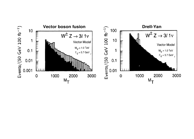
Turning now to the production of resonances in recent developments, the production at the LHC of a neutral KK excitation of the electroweak gauge bosons, generically called $Z^{\prime}$, in the context of a warped extra dimension model was studied by Agashe et al.[137]. They obtained that the Drell-Yan process is dominant over the VBF. The best discovery mode is $Z^{\prime}\rightarrow HZ\rightarrow b\bar{b}l^{+}l^{-}$, see Fig. 3. They conclude that a 2 (3) TeV $Z^{\prime}$ can be discovered with approximately 100 fb^-1 (1 ab^-1) integrated luminosity. Production of KK excitations of gauge bosons and its contribution to top quark pair production at the LHC was discussed in [176].

Figure 3: Cross section for $Z^{\prime}$ production at the LHC for different $Z^{\prime}$ masses, with the Drell-Yan and VBF processes shown separately (left panel). $Z^{\prime}$ mass reconstruction from $pp\rightarrow Z^{\prime}\rightarrow HZ\rightarrow b\bar{b}l^{+}l^{-}$ (right panel) (from [137]).

In the case of Higgsless models, an opposite situation occurs for the production of $W^{\prime}$ [36]. Due to the vanishing of fermionic couplings to the new vector resonance states, which guarantees a null correction to the electroweak precision parameters, the VBF is the dominant production process. A detailed study, including a complete leading order computation of the signal and relevant background, shows that with a 100 fb^-1 integrated luminosity the LHC will completely cover the parameter space of this model, with a 5 $\sigma$ discovery of $W^{\prime}$ up to a mass of 1.2 TeV, see Fig. 4.

Figure 4: Cross section for $W^{\prime}$ production at the LHC for different $W^{\prime}$ masses, with the associated $W^{\prime}Z$ and VBF processes shown separately (left panel).Significance for $W^{\prime}$ detection for the different modes (right panel) (from [221]).

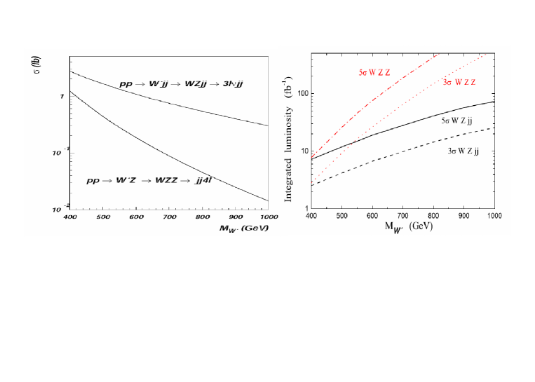
It is also interesting to point out that it could be possible to use gluon-gluon fusion Higgs production rate (and the Higgs decay rate to 2 photons) to discriminate among different models, such as UED and Gauge-Higgs unification models [222, 223, 224].

The next frontier in VBF is certainly the next-to-leading order (NLO) computations. A parton level Monte Carlo implementation of NLO QCD corrections to vector boson pair production via VBF was recently reported [225]. The implementation of new models in the same framework may be available in the near future.

See also [92, 226] for recent studies of strong $WW$ scattering.

4 RESONANCES IN A STRONGLY COUPLED EWSB SECTOR

4.1 Inspiration from low energy QCD

Low energy QCD (by low energy we mean $\sqrt{s}\ll m_{\rho}$) with two flavors is a theory of strongly coupled pions described by a chiral lagrangian (non-linear $\sigma$ model):

$${\cal L}=\frac{f_{\pi}^{2}}{4}Tr\left[\partial_{\mu}U\partial^{\mu}U^{\dagger}\right]$$ (17)

with $U=e^{i2\pi^{a}T^{a}/f_{\pi}}$ transforming as a $(2,2)$ under a global chiral symmetry $G=SU(2)_{L}\times SU(2)_{R}$:

$$U\rightarrow g_{R}Ug_{L}^{\dagger};\;\;g_{R}\in SU(2)_{R},\;\;g_{L}\in SU(2)_{L}.$$ (18)

This lagrangian is the lowest order term of an infinite expansion in an increasing number of derivatives of the field $U$. The pions are the Nambu-Goldstone bosons resulting from the spontaneous symmetry breaking $SU(2)_{L}\times SU(2)_{R}\rightarrow SU(2)_{V}$ generated by a non-zero vaccum expectation value $\langle U\rangle=1$.

It follows from the lagrangian (17) that $\pi\pi$ scattering amplitudes grow as $s/f_{\pi}^{2}$, as predicted by current algebra arguments. They violate $s-$wave perturbative unitarity when $\sqrt{s}\approx 4\pi f_{\pi}$. Higher derivative terms in the chiral lagrangian can delay the energy scale for unitarity violation.

There are several ad-hoc methods to unitarize $\pi\pi$ scattering but we will not dwell on them. In QCD, violation of perturbative unitarity points to the existence of $\pi\pi$ resonances, like the $\rho$ and $a_{1}$. Hence, one must extend the formalism of chiral perturbation theory to include these resonances in order to describe physics at energy scales $\sqrt{s}\approx m_{\rho}$. Possibly one of the most successful attempts to introduce resonances consists in describing them as dynamical gauge bosons of a local symmetry, as first proposed by Sakurai [227]. This idea led to the so-called hidden symmetry approach [228], where the masses of the resonances are generated via a Higgs mechanism. The hidden symmetry model can nicely accomodate features such as vector meson dominance and gauge invariance. It can also be used to describe resonances in a strongly coupled EWSB sector.

4.2 Strongly coupled EWSB sector

The EWSB sector in the SM is a gauged linear $\sigma$-model which can be nicely written as [194, 195]:

$${\cal L}_{SB}=\frac{1}{4}Tr\left[(D_{\mu}U)^{\dagger}D^{\mu}U\right]-\frac{1}{4}\lambda\left(\frac{1}{2}Tr\left[U^{\dagger}U\right]-v^{2}\right)^{2}$$ (19)

where

$$D_{\mu}U=\partial_{\mu}U+\frac{1}{2}igW_{\mu}^{i}\tau_{i}U-\frac{1}{2}ig^{\prime}Y_{\mu}U\tau_{3}.$$ (20)

In the limit $g^{\prime}\rightarrow 0$ this lagrangian has an additional global symmetry $G=SU(2)_{L}\times SU(2)_{R}$, with $U$ transforming as a $(2,2)$:

$$U\rightarrow e^{i\epsilon_{L}^{i}\tau_{i}/2}Ue^{-i\epsilon_{R}^{i}\tau_{i}/2}.$$ (21)

Electroweak symmetry is spontaneously broken by a non-zero vacuum expectation value $\langle U\rangle=v$, which generates masses for the electroweak gauge bosons. A so-called custodial global $SU(2)_{V}$ symmetry ($\epsilon_{L}=\epsilon_{R}$) survives, which is responsible for keeping the parameter $\rho=M_{W}^{2}/M_{Z}^{2}\cos\theta_{W}=1$ at tree level.

One way to introduce resonances from a strongly coupled sector in an effective lagrangian is to extend the SM global symmetry to a linearly realized $[SU(2)_{L}\times SU(2)_{R}]^{el}\times[SU(2)_{L}\times SU(2)_{R}]^{comp}$ symmetry. Here we are using the superscripts $(el)$ and $(comp)$ to denote the elementary and composite sectors respectively. The subgroup $[SU(2)_{L}\times U(1)_{X}]^{el}\times[SU(2)_{L}\times SU(2)_{R}]^{comp}$ will be gauged. The masses of all gauge bosons are generated via an extended Higgs mechanism. The SM Higgs can be part of the elementary sector (LDBESS model by Casalbuoni et al. [33, 229, 230]) or part of the composite sector (2-site composite Higgs model by Contino et al. [197]).

4.3 LDBESS model

Figure 5: Moose diagrams of the LDBESS model (left panel) and a 2-site composite Higgs model (right panel).

The scalar sector of the LDBESS model is given, as depicted on the moose diagram of Fig.5, by 3 sets of fields transforming under $[SU(2)_{L}\times SU(2)_{R}]^{el}\times[SU(2)_{L}\times SU(2)_{R}]^{comp}$ as

$$L\in(2,0,{\bar{2}},0)\; \Longrightarrow \;L\rightarrow g_{L}Lh^{\dagger}_{L}$$ (22)

$$R\in(0,2,0,{\bar{2}})\; \Longrightarrow \;R\rightarrow g_{R}Rh^{\dagger}_{R}$$ (23)

$$U\in(2,{\bar{2}},0,0)\; \Longrightarrow \;U\rightarrow g_{L}Ug_{R}^{\dagger},$$ (24)

where $g_{L,R}\in SU(2)_{L,R}^{el}$ and $h_{L,R}\in SU(2)_{L,R}^{comp}$. Notice that the Higgs field $U$ transforms under the elementary group.

The covariant derivatives acting on the scalar fields are (suppressing Lorentz indices):

$$DL = \partial L+ig_{2}\frac{\tau_{i}}{2}W^{i}L-ig^{*}_{L}L\frac{\tau_{i}}{2}V_{L}^{i}$$ (25)

$$DR = \partial R+ig_{1}\frac{\tau_{3}}{2}YR-ig^{*}_{R}R\frac{\tau_{i}}{2}V_{R}^{i}$$ (26)

$$DU = \partial U+ig_{2}\frac{\tau_{i}}{2}W^{i}U-ig_{1}U\frac{\tau_{3}}{2}Y,$$ (27)

where $W,Y,V_{L}$ and $V_{R}$ are the gauge bosons of the local $[SU(2)_{L}\times U(1)_{Y}]^{el}\times[SU(2)_{L}\times SU(2)_{R}]^{comp}$ symmetry. The couplings of the elementary sector are $g_{1}$ and $g_{2}$, whereas $g^{*}_{L}$ and $g^{*}_{R}$ are the couplings of the composite sector.

The scalar potential is chosen in such a way that $\langle L\rangle=\langle R\rangle=f\mathbf{1}_{2}$ and $\langle U\rangle=v\mathbf{1}_{2}$, with $f\gg v$, resulting in the symmetry breaking pattern

$$[2_{L}\times 1_{X}]^{el} \times [2_{L}\times 2_{R}]^{comp}\stackrel{{\scriptstyle\langle\tilde{L}\rangle=\langle\tilde{R}\rangle}}{{\longrightarrow}}[SU(2)_{L}\times U(1)_{Y}]^{SM}\ \ \stackrel{{\scriptstyle\langle\tilde{U}\rangle}}{{\longrightarrow}}U(1)_{em}$$ (28)

As usual, the scalar kinetic terms generate masses and mass-mixing terms for the gauge bosons:

$${\cal L}=\frac{1}{4}\textrm{Tr}\left[(D_{\mu}\tilde{U})^{\dagger}D^{\mu}\tilde{U}+(D_{\mu}\tilde{L})^{\dagger}D^{\mu}\tilde{L}+(D_{\mu}\tilde{R})^{\dagger}D^{\mu}\tilde{R}\right]$$ (29)

with the result:

$${\cal L}_{mass} = \frac{1}{8}\left[v^{2}\left(g_{2}^{2}W_{i}^{2}+g_{1}^{2}Y^{2}-2g_{2}g_{1}W_{3}Y\right)+f^{2}\left(g_{2}^{2}W_{i}^{2}+g^{*\,2}_{L}V_{L,i}^{2}-2g_{2}g^{*}_{L}W_{i}V_{L}^{i}\right)\right.$$

$$+ \left.f^{2}\left(g_{1}^{2}Y^{2}+g^{*\,2}_{R}V_{R,i}^{2}-2g_{1}g^{*}_{R}YV_{R}^{3}\right)\right]$$

Even in absence of EWSB ($v=0$), the $L$ link field induces a mixing between the elementary and the composite fields. The mass eigenstates are a mixture of elementary and composite fields. Diagonalizing the mass matrices after EWSB, we obtain the following spectrum

• Electrically charged sector

  • a composite massive $W_{h1}^{\pm}=V_{R}^{\pm}$ with a mass $m_{W_{h1}^{\pm}}=\frac{1}{2}g^{*}_{R}f$

  • a mostly composite massive $W_{h2}^{\pm}$ which is a combinaison of $W^{\pm}$ and $V_{L}^{\pm}$:

    $$W_{h2}^{\pm}=\sin\theta(1+r\cos^{2}\theta)W^{\pm}-\cos\theta(1-r\sin^{2}\theta)V_{L}^{\pm},$$ (30)

    with a mass given by

    $$M_{W_{h2}}^{2}=\frac{1}{4}g^{*\,2}_{L}f^{2}\left(\frac{1}{\cos^{2}\theta}+r\tan^{2}\theta+{\cal O}(v^{4}/f^{4})\right).$$ (31)

  • a mostly elementary light $W_{l}^{\pm}$ which is the linear combination orthogonal to $W_{h2}^{\pm}$

    $$W_{l}^{\pm}=\cos\theta(1-r\sin^{2}\theta)W^{\pm}+\sin\theta(1+r\cos^{2}\theta)V_{L}^{\pm},$$ (32)

    with a mass proportional the SM Higgs vev

    $$M_{W_{l}}^{2}=\frac{1}{4}g^{2}v^{2}\left(1-r\sin^{2}\theta+{\cal O}(v^{4}/f^{4})\right).$$ (33)

• Electrically neutral sector

  • a massless photon $\gamma=Y$.

  • a mostly elementary light $Z$ which is a linear combination of $W^{3}$ and $V_{L}^{3}$

    $$Z_{l}=\cos\theta(1-r\sin^{2}\theta)W^{3}+\sin\theta(1+r\cos^{2}\theta)V_{L}^{3},$$ (34)

    with a mass proportional to the SM Higgs vev and equal to $M_{W_{l}}$

  • a mostly composite heavy $Z_{h2}$ corresponding to the linear combination orthogonal to $Z_{l}$. Its mass is equal to $M_{W_{h2}}$

  • a composite heavy $Z_{h1}=V_{R}^{3}$ with a mass $m_{Z_{h1}^{\pm}}=\frac{1}{2}g^{*}_{R}f$.

The mixing angle $\theta$ corresponds to the ratio of the gauge couplings of the elementary and composite sectors

$$\sin\theta=\frac{g_{2}}{\sqrt{g_{2}^{2}+g_{L}^{*\,2}}}.$$ (35)

It measures the amount of compositeness in the massless gauge bosons before EWSB. $g$ is the gauge coupling of the low-energy SM $SU(2)$ gauge coupling

$$g^{2}=\frac{g_{2}^{2}g_{L}^{*\,2}}{g_{2}^{2}+g_{L}^{*\,2}},$$ (36)

after the breaking $SU(2)^{el}\times SU(2)^{comp}$ to $SU(2)_{L}^{SM}$. Note that $g\simeq g_{2}$ if the composite sector is strongly coupled ($g^{*}_{L}\gg g_{2}$). Finally, the parameter $r$ measures the mass gap between the light and the heavy states

$$r=\frac{g^{2}v^{2}}{g_{L}^{*\,2}f^{2}}\simeq\frac{M_{W_{l}}^{2}}{M_{W_{h2}}^{2}}.$$ (37)

We have neglected here the coupling $g_{1}$ of the elementary $U(1)$ gauge group. Turning it on will induce a mixing of $V^{3}_{L},V^{3}_{R},W^{3}$ and $Y$.

Trilinear couplings between the light and the heavy states arise from the gauge kinetic terms,

$${\cal L}_{gauge}=\sum_{W,Y,V_{L},V_{R}}\frac{1}{2}\textrm{Tr}\left[F_{\mu\nu}^{2}\right].$$ (38)

For instance, we obtain the coupling

$$g_{Z_{h1}W^{+}_{l}W^{-}_{l}}=g\,r\sin\theta\cos\theta.$$ (39)

Notice that the coupling is suppressed by a factor $r$ and that, in the absence of symmetry breaking, this coupling vanishes.

This model can also be extended to include more resonances by simply introducing more copies of $[SU(2)_{L}\times SU(2)_{R}]^{comp}$ or $[SU(3)_{c}\times SU(2)_{L}\times SU(2)_{R}]^{comp}$ if color octet vector bosons (gluon resonances) are present in the spectrum. However, the basic idea is the one shown above. Notice that in the case of gluon resonances, their coupling to gluons would vanish since the color symmetry is unbroken, as pointed out in [231].

4.4 A 2-site composite Higgs model

The basic difference between the LDBESS model and a 2-site composite Higgs is that the Higgs is now part of the strong sector and interacts directly with the composite gauge bosons. So

$$U\in(0,0,2,\bar{2})\;\Longrightarrow\;U\rightarrow h_{L}Uh_{R}^{\dagger}$$ (40)

and

$$DU=\partial U+ig^{*}_{L}\frac{\tau_{i}}{2}V_{L}^{i}U-ig^{*}_{R}U\frac{\tau_{i}}{2}V_{R}^{i},$$ (41)

in the notation adopted in the previous section. One still keeps $\langle L\rangle=\langle R\rangle=f$ and $\langle U\rangle=v$. Consequently we now have the mass-mixing lagrangian given by:

$${\cal L}_{mass} = \frac{1}{8}\left[v^{2}\left(g^{*\,2}_{L}V_{L,i}^{2}+g^{*\,2}_{R}V_{R,i}^{2}-2g^{*}_{L}g^{*}_{R}V^{i}_{L}V^{i}_{R}\right)+f^{2}\left(g_{2}^{2}W_{i}^{2}+g^{*\,2}_{L}V_{L,i}^{2}-2g_{2}g^{*}_{L}W_{i}V_{L}^{i}\right)\right.$$

$$+ \left.f^{2}\left(g_{1}^{2}Y^{2}+g^{*\,2}_{R}V_{R,i}^{2}-2g_{1}g^{*}_{R}YV_{R}^{3}\right)\right]$$

As before, the mass eigenstates are linear combinations of elementary and composite states. Diagonalizing the mass mixing terms, we easily obtain the spectrum after EWSB. For example, in the electrically charged sector, we get two massive $W^{\pm}_{h,1-2}$ with masses given by

$$m_{W^{\pm}_{h1}}^{2}=\frac{1}{4}g^{*\,2}_{R}f^{2}+\frac{1}{4}g^{*\,2}_{R}v^{2}+\mathcal{O}(v^{4}/f^{2})$$ (42)

$$m_{W^{\pm}_{h2}}^{2}=\frac{1}{4}g^{*\,2}_{L}f^{2}\left(\frac{1}{\cos^{2}\theta}+r\,\textrm{cotan}^{2}\theta+{\cal O}(v^{4}/f^{4})\right).$$ (43)

and one light $W_{l}^{\pm}$ whose mass is proportional to the Higgs vev and that can be identified with the SM $W^{\pm}$

$$M_{W_{l}}^{2}=\frac{1}{4}g^{2}v^{2}+{\cal O}(v^{4}/f^{2}).$$ (44)

As for the LDBESS model, $g$ is the gauge coupling of the low-energy SM $SU(2)$ gauge coupling

$$g^{2}=\frac{g_{2}^{2}g_{L}^{*\,2}}{g_{2}^{2}+g_{L}^{*\,2}},$$ (45)

after the breaking $SU(2)^{el}\times SU(2)^{comp}$ to $SU(2)_{L}^{SM}$ at the scale $f$ and the mixing angle $\theta$ is the ratio of the gauge couplings of the elementary and composite sectors

$$\sin\theta=\frac{g_{2}}{\sqrt{g_{2}^{2}+g_{L}^{*\,2}}}.$$ (46)

Finally, $r$ is the mass gap between the light and the heavy states

$$r=\frac{g^{2}v^{2}}{g_{L}^{*\,2}f^{2}}\simeq\frac{M_{W_{l}}^{2}}{M_{W_{h2}}^{2}}.$$ (47)

The spectrum is the same as in the LDBESS model up to differences of $\mathcal{O}(v^{2}/f^{2})$ in the heavy sector. Still, these differences have big effects in the couplings of the Higgs boson to the heavy resonances. These couplings can be simply obtained by substituting $v$ by $v+h$ in the lagrangian: therefore, in the LDBESS model the Higgs coupling to $W^{\pm}_{h2}$ are reduced two powers of the compositeness angle $\theta$, while in the composite Higgs model, the coupling is enhanced by the same factor.

Part 13 Vector-like quarks: a toolkit for experimenters

J. Santiago

In four space-time dimensions, Dirac fermions can be decomposed into left- and right-handed chiralities, $\psi=\psi_{L}+\psi_{R}$, with $\psi_{L,R}=(1\mp\gamma^{5})/2\,\psi$. Chiral fermions, for which the two components have different charges under the electroweak $SU(2)_{L}\times U(1)_{Y}$ gauge group, have masses proportional to the electroweak symmetry breaking (EWSB) scale ($v\sim 174$ GeV) and are therefore expected to be relatively light, $m_{\mathrm{chiral}}=\lambda v\lesssim v$. They can only be made heavy at the expense of introducing a large dimensionless coupling $\lambda\gg 1$, thereby inducing large one loop corrections to electroweak observables (they do not decouple). Thus, new chiral fermions are quite constrained experimentally from electroweak precision tests (EWPT). If the fermions are vector-like (the two chiralities have the same quantum numbers) we can write down a gauge invariant (Dirac) mass that is unrelated to the EWSB scale. They can therefore be naturally heavier than $v$ without introducing large dimensionless couplings. As the Dirac mass becomes large, their low energy effects become negligible (decoupling) and EWPT impose no constraints. Furthermore, new vector-like fermions are a very common prediction of theories beyond the Standard Model (SM), from Kaluza-Klein modes in models with extra dimensions to partners of the SM fermions in little Higgs models, or members of extended multiplets in GUT theories.

For their relevance to LHC physics, we will restrict ourselves to vector-like quarks, transforming as triplets under the $SU(3)$ gauge group. We will also consider only the case of new quarks that can sizably mix (through mass terms) with SM quarks, generating flavour changing electroweak processes that can lead to interesting signatures at the LHC. Finally, we will assume that a (relatively) light SM-like Higgs boson (doublet under $SU(2)_{L}$) exists in the spectrum and is the main source of EWSB.

1 HOW TO COMPUTE THE RELEVANT FEATURES: MASSES AND COUPLINGS

New vector-like quarks with sizable mixings with the SM quarks cannot have arbitrary quantum numbers. They can only couple in a gauge invariant way to a SM quark and the Higgs, which gives only the seven distinct possibilities shown in Table 1.

Table 1: Vector-like quark multiplets $Q$ mixing with the SM quarks through Yukawa couplings. The electric charge is $Q=T_{3}+Y$.

$Q$	$U$	$D$	$\begin{pmatrix}U\cr D\end{pmatrix}$	$\begin{pmatrix}X\cr U\end{pmatrix}$	$\begin{pmatrix}D\cr Y\end{pmatrix}$	$\begin{pmatrix}X\cr U\cr D\end{pmatrix}$	$\begin{pmatrix}U\cr D\cr Y\end{pmatrix}$
isospin	0	0	${1}/{2}$	${1}/{2}$	${1}/{2}$	1	1
hypercharge	${2}/{3}$	$-{1}/{3}$	${1}/{6}$	${7}/{6}$	$-{5}/{6}$	${2}/{3}$	$-{1}/{3}$

Given these possibilities, the question is, how do we get the relevant features of the model in order to study it at colliders. Or said otherwise, what are the masses and couplings of these new quarks? The aim of this short review is to present the general algorithm to compute these relevant features and to exemplify it in a particular case that will be further explored below. The general Lagrangian can be written, in the current eigenstate basis (i.e. in terms of fermions with well defined $SU(2)_{L}\times U(1)_{Y}$ quantum numbers), as

$$\mathcal{L}_{l}+\mathcal{L}_{h}+\mathcal{L}_{lh},$$ (1)

where $\mathcal{L}_{l}$ is the SM Lagrangian, $\mathcal{L}_{h}$, contains the kinetic, Dirac mass terms (that can always be taken diagonal) and Yukawa couplings involving only the (heavy) vector-like quarks, and finally $\mathcal{L}_{lh}$ contains the (linear) mass (and Yukawa) mixing between SM and vector-like quarks. The general expressions for these Lagrangians can be found in Ref. [232]. In order to obtain the properties of the physical particles (i.e. those with a well defined mass) we have to diagonalize the corresponding mass matrices that are contained in $\mathcal{L}_{h}+\mathcal{L}_{lh}$. Due to the unbroken electromagnetic $U(1)_{Q}$ gauge invariance, the mass matrix will be block diagonal according to the charges of the different fields,

$$\mathcal{L}_{\mathrm{mass}}=\sum_{Q}\bar{\psi}^{(0)Q}_{L}\mathcal{M}_{Q}\psi^{(0)Q}_{R}+\mathrm{h.c.},$$ (2)

where $\psi^{(0)Q}_{L,R}$ is a vector that contains the $n_{Q}$ quarks with charge $Q$ and $\mathcal{M}^{Q}$ is a $n_{Q}\times n_{Q}$ matrix. The overscript $(0)$ denotes current eigenstates. We can then diagonalize each block with two unitary matrices $U^{Q}_{L,R}$,

$$(U^{Q}_{L})^{\dagger}\mathcal{M}_{Q}U^{Q}_{R}=\mathcal{D}_{Q},$$ (3)

with $\mathcal{D}_{Q}$ a diagonal matrix containing the masses of the physical particles. $U^{Q}_{L,R}$ can be computed as the unitary matrices that diagonalize the mass matrix squared, $(U_{L}^{Q})^{\dagger}\mathcal{M}_{Q}\mathcal{M}_{Q}^{\dagger}U_{L}^{Q}=(U^{Q}_{R})^{\dagger}\mathcal{M}_{Q}^{\dagger}\mathcal{M}_{Q}U^{Q}_{R}=\mathcal{D}_{Q}^{2}$. Once we have computed the rotation matrices $U^{Q}_{L,R}$, we only have to replace in the gauge and Yukawa couplings the mass eigenstates in terms of the physical quarks,

$$\psi^{(0)Q}_{L,R}=U_{L,R}^{Q}\psi^{Q}_{L,R},$$ (4)

where $\psi^{Q}_{L,R}$ are now the physical states. This final step will have two main implications. First, it will modify the SM quark couplings to the electroweak gauge bosons and the Higgs, and second it will introduce off-diagonal (electroweak) gauge and Yukawa couplings between heavy and SM quarks. In general, the first effect strongly contraints large mixing of vector-like quarks with first and second generation quarks (as their couplings have been measured to agree very well with the SM prediction).  Only mixing with the top is at present poorly constrained and could be large. If the new vector-like quarks play a role in the resolution of the hierarchy problem, it is indeed natural for them to be relatively light and to mix sizably with the top. Note that in this case they might induce sizable corrections at loop level to precision observables, most notably the $T$ parameter and the $Z\bar{b}b$ coupling, that should be checked in particular models [233, 234, 235].

Let us make this procedure more explicit with one relevant example whose phenomenology will be further studied in this report. In particular, we will consider an extension of the SM with two vector-like quark doublets, $q_{L,R}=(q^{u},q^{d})^{\mathrm{T}}_{L,R}$ and $\chi_{L,R}=(\chi^{u},\chi^{d})^{\mathrm{T}}_{L,R}$, with hypercharges $Y_{\chi}=7/6$ and $Y_{q}=1/6$, respectively. The electric charge of the different components are given by $Q=T_{3}+Y$ ($Q_{\chi^{u}}=5/3$, $Q_{q^{u}}=Q_{\chi^{d}}=2/3$ and $Q_{q^{d}}=-1/3$). Note in particular the exotic charge of $\chi^{u}$. For simplicity, we will also assume that these two new quark doublets can only mix with the top but not with the bottom or any other light quark. This example is motivated by recent ideas using a subgroup of the custodial symmetry to protect large corrections to the $Z\bar{b}_{L}b_{L}$ coupling [107] for which these simplifying assumptions are naturally realized. This mechanism has been successfully implemented in composite Higgs [234, 236, 235, 237, 238] and Higgsless models [239] in warped extra dimensions.

The mass Lagrangian for the charge $2/3$ quarks (the other ones do not have any mass mixings and are therefore mass eigenstates) can be written as,

$$\mathcal{L}=\begin{pmatrix}\bar{t}_{L}^{(0)}&\bar{q}_{L}^{u(0)}&\bar{\chi}_{L}^{d(0)}\end{pmatrix}\begin{pmatrix}m_{t}&0&0\\ m_{q,t}&M_{q}&0\\ m_{\chi,t}&0&M_{\chi}\end{pmatrix}\begin{pmatrix}t_{R}^{(0)}\\ q_{R}^{u(0)}\\ \chi_{R}^{d(0)}\end{pmatrix}+\mathrm{h.c.}\,.$$ (5)

EWSB masses, which are proportional to the Higgs vev, are denoted with a lower case $m$ whereas Dirac masses, that can be arbitrarily larger than $v$ are denoted by a capital $M$. The hierarchy between these two types of masses, allows us to diagonalize the mass matrix perturbatively, in a power expansion of $m/M\ll 1$ in order to obtain simple analytic expressions for the masses and couplings of the physical quarks. For instance, to leading order in $m/M$, we have

$$t^{(0)}_{R}\approx t_{R}+\frac{m_{q,t}}{M_{q}}q^{u}_{R}+\frac{m_{\chi,t}}{M_{\chi}}\chi^{d}_{R},\quad q^{u(0)}_{R}\approx q^{u}_{R}-\frac{m_{q,t}}{M_{q}}t_{R},\quad\chi^{d(0)}_{R}\approx\chi^{d}_{R}-\frac{m_{\chi,t}}{M_{\chi}}t_{R},$$ (6)

where fields without the $(0)$ superscript are physical (mass eigenstate) fields. All other fields are not modified (i.e. they are already mass eigenstates) at this order. Now we only have to introduce these rotations in the gauge and Yukawa couplings to obtain the couplings among the physical fields. The couplings to the $Z$ are, in the current and mass eigenstate basis, respectively

$$\mathcal{L}^{Z} = -\frac{g}{2c_{W}}Z_{\mu}[\bar{q}_{R}^{u(0)}\gamma^{\mu}q_{R}^{u(0)}-\bar{\chi}_{R}^{d(0)}\gamma^{\mu}\chi_{R}^{d(0)}-2s_{W}^{2}J^{R\mu}_{2/3}]$$ (7)

$$= \mathcal{L}^{Z}_{0}-\frac{g}{2c_{W}}Z_{\mu}\left[\frac{m_{\chi,t}}{M_{\chi}}\bar{t}_{R}\gamma^{\mu}\chi^{d}_{R}-\frac{m_{q,t}}{M_{q}}\bar{t}_{R}\gamma^{\mu}q^{u}_{R}+\mathrm{h.c.}\right]+\mathcal{O}\left(\frac{m^{2}}{M^{2}}\right),$$

where $J^{R\mu}_{2/3}=(2/3)(\bar{t}_{R}^{(0)}\gamma^{\mu}t^{(0)}_{R}+\bar{q}_{R}^{u(0)}\gamma^{\mu}q_{R}^{u(0)}+\bar{\chi}_{R}^{d(0)}\gamma^{\mu}\chi_{R}^{d(0)})=(2/3)(\bar{t}_{R}\gamma^{\mu}t_{R}+\bar{q}_{R}^{u}\gamma^{\mu}q_{R}^{u}+\bar{\chi}_{R}^{d}\gamma^{\mu}\chi_{R}^{d})$ is the electromagnetic current for the RH charge $2/3$ quarks and $\mathcal{L}^{Z}_{0}$ is equal to the original Lagrangian with the replacement $\psi^{(0)}\to\psi$. Similarly we obtain, for the charge currents

$$\Delta\mathcal{L}^{W}=\mathcal{L}^{W}-\mathcal{L}^{W}_{0}=\frac{g}{\sqrt{2}}W^{+}_{\mu}\left[\frac{m_{q,t}}{M_{q}}\bar{t}_{R}\gamma^{\mu}q^{d}_{R}+\frac{m_{\chi,t}}{M_{\chi}}\bar{\chi}^{u}_{R}\gamma^{\mu}t_{R}\right]+\mathrm{h.c.}+\mathcal{O}\left(\frac{m^{2}}{M^{2}}\right),$$ (8)

and Yukawa couplings

$$\Delta\mathcal{L}^{H}=\mathcal{L}^{H}-\mathcal{L}^{H}_{0}=\frac{H}{v}[m_{q,t}\bar{q}^{u}_{L}t_{R}+m_{\chi,t}\bar{\chi}^{d}_{L}t_{R}+\mathrm{h.c.}]+\mathcal{O}\left(\frac{m^{2}}{M^{2}}\right).$$ (9)

Diagonal couplings and masses are only modified at $\mathcal{O}(m^{2}/M^{2})$ [240] which, for the purpose of their collider implications can usually be considered a negligible correction. (Of course if the vector-like quark masses are close to the electroweak scale, $M\sim v$, this expansion breaks down and a full numerical diagonalization would be required). Using these couplings we can compute the decay width of the different heavy quarks. The result is extremely simple in the large $M$ limit, in which we obtain

$$\Gamma(\chi^{u}\to Wt)\approx 2\Gamma(q^{u}\to Zt)\approx 2\Gamma(q^{u}\to Ht)\approx\frac{g^{2}}{64\pi}\frac{m_{q,t}^{2}M_{q}}{M_{W}^{2}},$$ (10)

$$\Gamma(q^{d}\to Wt)\approx 2\Gamma(\chi^{d}\to Zt)\approx 2\Gamma(\chi^{d}\to Ht)\approx\frac{g^{2}}{64\pi}\frac{m_{\chi,t}^{2}M_{\chi}}{M_{W}^{2}}.$$ (11)

Note the $2:1:1$ pattern of decays into $W,Z,H$ as predicted by the Equivalence Theorem. This means that, for heavy vector-like quarks, the decay is mainly into longitudinal gauge bosons (or equivalently in the Goldstone bosons in a gauge other than the unitary one).

Vector-like quarks can be pair or singly produced. Pair production is governed by QCD and is therefore model-independent. There is a very strong suppression at large masses which makes the reach at the LHC $\sim 1-2$ TeV [192, 241]. However, pair production can give rise to spectacular signatures. For instance, pair production of $\chi^{u}$ or $q^{d}$ results in a final state with four $W$ plus two $b$ quarks. An analysis of the reach in that case, using like-sign leptons will be discussed below. Single production occurs through the off-diagonal couplings between SM and heavy quarks. Although it is model-dependent, the suppression at large masses is milder than in pair production. Thus, if the new quarks mix sizably with light quarks (including the bottom), single production can give a better reach than pair production [242].

2 CONCLUSIONS

Vector-like quarks are a common prediction of models of new physics. They are in general compatible with EWPT and can give rise to spectacular signals at the LHC. We have reviewed the tools needed to compute their collider implications (masses and couplings) and discussed a particular example relevant for realistic composite Higgs and Higgsless models. Other possibilities have been discussed elsewhere, with special emphasis on the case of a vector-like singlet (for a recent review see [243], page 72, and references there in).

ACKNOWLEDGEMENTS

We thank R. Contino, B. Dobrescu, C. Grojean and especially E. Pontón for helpful comments. This work is supported by SNSF under contract 200021-117873.

blabla

Nonleptonic Final States

Part 14 Top-partner mass reconstruction by using jets

M.M. Nojiri and M. Takeuchi

1 TOP PARTNERS IN THE LITTLEST HIGGS MODEL WITH T PARITY

1.1 Productions and decays

We consider the Littlest Higgs model with T parity (LHT). In the following, we assume the top partner is the lightest in the SM fermions’ partners. The top partner may be produced in pairs and decays at LHC as,

$$pp\rightarrow T_{-}\overline{T}_{-}\rightarrow t\bar{t}A_{H}A_{H}\rightarrow bW^{+}\bar{b}W^{-}A_{H}A_{H}\rightarrow 6j+E{\!\!\!/}_{T}.$$ (1)

This process is similar to the top squark ($\tilde{t}$) production process in the MSSM. However, the top partner production cross section is larger than that of top squarks when the masses are same, because the top partner is a fermion. At the LHC, the $T_{-}\overline{T}_{-}$ production cross section is 0.171 pb for the top partner mass $m_{T_{-}}$ set to 800 GeV. Once the top partner is produced, it decays into top and the heavy photon $A_{H}$ (We set to 150GeV). The branching ratio is 100% when the top partner is the next lightest T-odd particle. To identify this process, it is important to identify two tops and missing transverse momentum $E{\!\!\!/}_{T}$.

To simulate the top partner reconstruction we generated 8,550 $\tilde{t}\tilde{t}^{\ast}$ events with HERWIG6.5 (expected number of events for 50fb^-1). We use a similar MSSM model point instead of the LHT for the event generation. The distribution of production and decay is almost correct except for the spin correlations of $T_{-}$ decays, so we do not simulate top partner polarization effects but top polarization is taken into account. The main source of SM background is $t\bar{t}$ events, whose production cross section is 463 pb at tree level. We also generated 4,630,000 $t\bar{t}$ events (for 10fb^-1). When we compare signal and background distributions, we simply multiply $t\bar{t}$ distributions by a factor of 5. We ignore the $t\bar{t}Z$ background because this can be calibrated with $t\bar{t}Z(\rightarrow l^{+}l^{-})$ events easily.

The process was already analysed in [244], where AcerDET1.0 [245] was used for the detector simulation and jet reconstruction. We also use AcerDET1.0 for the detector simulation. In addtion to that, we interfaced the calorimeter information to FastJet2.2beta [246] which allows us to compare different jet reconstruction algorithms (kt, Cambridge, SISCone). To compare the four jet algorithms under the same conditions (in Sec 2), we switch off jet energy smearing of AcerDET. In this section, we only show the results with the Cambridge algorithm.

1.2 Event selection and Top mass reconstruction

We apply successive cuts to select $T_{-}\overline{T}_{-}$ events, the summary of the cuts is shown in Table 1. First, we imposed the standard cut to collect events related with new physics,

$$E{\!\!\!/}_{T}\geq 200{\rm GeV\ and}\ E{\!\!\!/}_{T}\geq 0.2M_{\rm eff},\ \ n_{\rm lepton}=0.$$ (2)

The lepton cut is for dropping $t\bar{t}$ production events, in which large $E\!\!\!/_{T}$ is dominantly caused by neutrinos from the leptonic decay of top. We do not assume any b tagging, because for the given kinematics jets are very collinear with each other, and the $b$ tagging efficiency has not been studied in that case.

We applied the hemisphere analysis to find top candidates[247]. Each of the jets was assigned to hemispheres which were defined as follows;

$$\forall i\in H_{1},j\in H_{2}\ \ \ \ \ \ \ \ d(p_{H_{1}},p_{i})\leq d(p_{H_{2}},p_{i}){\rm\ and\ }d(p_{H_{2}},p_{j})\leq d(p_{H_{1}},p_{j}).$$ (3)

$$\ \ \ \ \ d(p_{1},p_{2})\equiv\frac{(E_{1}-|\mathbf{p}_{1}|\cos\theta)E_{1}}{(E_{1}+E_{2})^{2}}\ \ \ \ (\theta\ {\rm is\ the\ angle\ between\ }\mathbf{p}_{1}\ {\rm and}\ \mathbf{p}_{2}).$$ (4)

Here, $p_{H_{j}}\equiv\sum_{i\in H_{j}}p_{i}$, and we required both hemispheres’ transverse momenta to be larger than a threshold,

$$p_{T,H_{1}},p_{T,H_{2}}>200{\rm GeV}.$$ (5)

Top quarks from $T_{-}\overline{T}_{-}$ production are highly boosted. Therefore decay products from two top quarks are correctly grouped into two hemispheres with high probability. We analysed the events in which each hemisphere has up to 3 jets to drop contribution from other QCD jets.

The distributions of invariant masses of hemispheres ($m_{P_{H}}\equiv\sqrt{p_{H}^{2}}$) for the $T_{-}\overline{T}_{-}$ and $t\bar{t}$ events are shown in the Fig 3. We can see the top mass peak both for the $T_{-}\overline{T}_{-}$ and $t\bar{t}$ events in the $H_{1}$. On the other hand, the top mass is not well reconstructed in the $H_{2}$ for $t\bar{t}$ events. This is because at least one of tops must decay leptonically to make large $E\!\!\!/_{T}$. Two dimensional scattering plots of $m_{P_{H1}}$ vs. $m_{P_{H2}}$ are also shown in Fig 3. We regard a hemisphere’s momentum as the top momentum in this paper if its mass is consistent with the top mass ($150$GeV $<m_{P_{H}}<190$GeV). The matching of a hemisphere’s momentum with the parton momentum is discussed in Section 2.1.

	generated	$E{\!\!\!/},M_{\rm eff}$ cut	$n_{\rm lep}=0$	$p_{T,H}$ cut	$n_{{\rm jet},H}\!\leq\!3$	$m_{P_{H1}}$	$m_{P_{H2}}$	both $m_{P_{H}}$	relaxed $m_{P_{H}}$
$T_{-}\overline{T}_{-}$	8,550	6,590	4,384	2276	1433	437	380	118	708
$t\bar{t}$	23,150,000	199,640	88,540	9475	6835	2105	765	235	1835
S/$\sqrt{N}$	1.777	14.75	14.73	23.38	17.33	9.525	13.73	7.70	16.53

Table 1: Summary of the cuts. The number of events are for $\int\!\!dt{\cal L}=50\,$ fb^-1. $p_{T,H}$ denotes the cuts that requires both hemispheres’ momenta $p_{T,H_{1}},p_{T,H_{2}}>200$GeV. $m_{P_{Hi}}$ denotes the cuts that the hemisphere $i$’s momentum is consistent with top mass ($150$GeV $<m_{P_{H}}<190$GeV). The relaxed $m_{P_{H}}$ cut denotes that both hemispheres’ momenta satisfy $50$GeV $<m_{P_{H}}<190$GeV.

Figure 1: The distributions of invariant masses of a) $H_{1}$ for the $T_{-}\overline{T}_{-}$ events, b) $H_{2}$ for the $T_{-}\overline{T}_{-}$ events, c) $H_{1}$ for the $t\bar{t}$ events, d) $H_{2}$ for the $t\bar{t}$ events.

Figure 2: $m_{P_{H1}}$ vs. $m_{P_{H2}}$ for $T_{-}\overline{T}_{-}$ (upper figure) and for $t\bar{t}$ (lower figure). Cambridge algorithm is used for Jet reconstruction.

Figure 3: The $m_{T2}$ distribution for the Cambridge algorithms, where proper $m_{\tilde{\chi}^{0}_{1}}=150$ GeV is used. The dashed line shows for events with $150{\rm GeV}<m_{P_{Hi}}<190{\rm GeV}$ The solid line shows for events with $50{\rm GeV}<m_{P_{Hi}}<190{\rm GeV}$. The endpoints are 790.95 GeV for nominal $m_{A_{H}}$. ($m_{T_{-}}=800$ GeV).

1.3 Measurement of the end point of $m_{T2}$ distribution.

To extract the mass of $T_{-}$, we used the Cambridge $m_{T2}$ variable [248]. This variable is considered in events like $\zeta\zeta^{\prime}\to(a\alpha)(b\beta)$, where we assume $\zeta$ and $\zeta^{\prime}$ have the same mass $m_{\zeta}$, $a$ and $b$ are visible objects, and $\alpha$ and $\beta$ are invisible particles and have the same mass $m_{\tilde{\chi}^{0}_{1}}$. In the events, the $m_{T2}$ variable is defined as follows:

$$\!\!\!\!m_{T2}^{2}(\mathbf{p}_{T}^{a},\mathbf{p}_{T}^{b},\mathbf{p}{\!\!\!/}_{T};m_{\tilde{\chi}^{0}_{1}})\equiv\min_{\mathbf{p}{\!\!\!/}_{T}^{\alpha}+\mathbf{p}{\!\!\!/}_{T}^{\beta}=\mathbf{p}{\!\!\!/}_{T}}\left[\max\left\{m_{T}^{2}(\mathbf{p}_{T}^{a},\mathbf{p}{\!\!\!/}_{T}^{\alpha};m_{\tilde{\chi}^{0}_{1}}),m_{T}^{2}(\mathbf{p}_{T}^{b},\mathbf{p}{\!\!\!/}_{T}^{\beta};m_{\tilde{\chi}^{0}_{1}})\right\}\right].$$ (6)

Here, the transverse mass $m_{T}$ is defined as $m_{T}^{2}(\mathbf{p}_{T}^{a},\mathbf{p}{\!\!\!/}_{T}^{\alpha};m_{\tilde{\chi}^{0}_{1}})\equiv m_{a}^{2}+m_{\tilde{\chi}^{0}_{1}}^{2}+2\left[E_{T}^{a}E{\!\!\!/}_{T}^{\alpha}-\mathbf{p}_{T}^{a}\mathbf{p}{\!\!\!/}_{T}^{\alpha}\right].$ By the definition, the $m_{T2}$ variable is a function of $m_{\tilde{\chi}^{0}_{1}}$, and satisfies the condition $m_{T2}(m_{\tilde{\chi}^{0}_{1}})\leq m_{\zeta}$. Then we can measure $m_{\zeta}$ by measuring the upper endpoint of the $m_{T2}$ distribution.

For our purpose, visible particles are two top quarks and invisible particles are two $A_{H}$. We may regard hemispheres’ momenta as top momenta for the hemisphere whose masses are $150{\rm GeV}<m_{P_{Hi}}<190{\rm GeV}$. However, there are not enough events left under this cut. Therefore we use a relaxed criterion $50{\rm GeV}<m_{P_{Hi}}<190{\rm GeV}$. Indeed, when $m_{P_{H}}$ is less than $m_{t}$, all of the top decay products do not contribute to the hemisphere reconstruction due to the minimum jet energy cuts. The endpoint of $m_{T2}$ does not change because $m_{T}$ is always underestimated compared to the true $m_{T}$. This is easy to understand if you consider the system of a neutralino and other sources of missing momenta ( for example neutrino ) as one invisible particle. The invisible particle mass ($m_{\rm invisible}$) is always larger than the neutralino mass which results in $m_{T2}(m_{\tilde{\chi}^{0}_{1}})\leq m_{T2}(m_{\rm invisible})\leq m_{\zeta}$.

The $m_{T2}$ distribution is shown in Fig 3, where the nominal value $m_{\tilde{\chi}^{0}_{1}}=150$ GeV is used for the calculation of $m_{T2}$. We show only the region of $m_{T2}>350{\rm GeV}$. The $t\bar{t}$ events have low $m_{T2}$ values, so we can neglect the BG to fit the endpoint. The dashed lines show the $m_{T2}$ distributions for events with $150{\rm GeV}<m_{P_{Hi}}<190{\rm GeV}$ and have the same endpoint as those with the relaxed criterion of $50{\rm GeV}<m_{P_{Hi}}<190{\rm GeV}$ (solid line). This fact supports the validity to relax the criterion to determine the endpoint. We fitted the distribution near the endpoint by a linear function and obtained $m_{T2}^{max}=790.95$ GeV. This value is consistent with the proper value $m_{T_{-}}=800$ GeV.

It is not possible to determine the top partner mass itself unless the $A_{H}$ mass is determined. If we assume the $A_{H}$ thermal relic density is consistent with the dark matter density in our universe, $m_{A_{H}}$ is related to the Higgs mass ($m_{H}$) so that it is determined with two fold ambiguity [244].

2 COMPARISON AMONG JET RECONSTRUCTION ALGORITHMS

We now make a comment on the dependence on the jet reconstructing algorithm. Four algorithms for jet reconstruction (Simple cone, kt, Cambridge, SISCone) are used in the following analysis. For this study, we interfaced FastJet2.2beta [246] to AcerDET1.0. The energy deposits in calorimeter cells are regarded as ”particle momentum”. Cone sizes (or the counterparts for clustering algorithms) $R$ are chosen as 0.4 and overlap parameter $f$ as 0.5 for SISCone. Simple cone denotes the algorithm used in AcerDET1.0.

2.1 Invariant mass distributions

The results are summarized in Table 2. Acerdet has an option to calibrate jet momenta, therefore both calibrated and non-calibrated numbers are given for the simple cone algorithm in the table. The calibrated result is shown in the figures.

For $T_{-}\overline{T}_{-}$ events	$E{\!\!\!/},M_{\rm eff}$ cut	$n_{{\rm jet},H}\leq 3$	$m_{P_{H1}}$	$m_{P_{H2}}$	both $m_{P_{H}}$	relaxed $m_{P_{H}}$	$m_{T2}$ endpoint
Simple Cone (calibrated)	6673	945	306	326	110	439	795.69 GeV
(not calibrated)	6673	1213	283	323	82	545	779.37 GeV
kt	6673	1436	444	384	105	604	780.62 GeV
Cambridge	6673	1433	437	380	118	621	790.95 GeV
SISCone	6673	1656	512	437	150	608	803.67 GeV

Table 2: Summary of the cuts for various jet algorithms. cut is the same as Table 1.

The distributions of $m_{P_{H1}}$ are shown in Fig 6. The shaded regions denote that the hemisphere’s invariant mass is consistent with $m_{t}$ ($150{\rm GeV}<m_{P_{H}}<190{\rm GeV}$). The peak for the Simple cone algorithm is dull and has a broad tail and the position of the peak is located below $m_{t}$. This is because AcerDET takes massless jets. Therefore the probability to find the jets consistent with the top mass is relatively low among the four algorithms. The acceptance becomes worse as the lower bound of an invariant mass cut for $m_{P_{H}}$ is increased. If the other jet definitions are feasible in the LHC environment, the reconstruction efficiency can be increased significantly. On the other hand, the endpoints of the $m_{T2}$ distributions are 795.69 (779.37) GeV (Simple cone), 780.62 GeV (kt), 790.95 GeV (Cambridge), 803.67 GeV (Siscone) respectively. The dependence on jet algorithms is not severe for this analysis.

Fig 6 shows the deviation of the hemisphere momentum from the true top quark momentum $(\Delta p_{T})/p_{T}$. We selected signal events with 150 GeV$<m_{P_{H1}}<$ 190 GeV for the Simple cone and Cambridge algorithms. They are mostly distributed in a $\pm 5$% region. We can see the $(\Delta p_{T})/p_{T}$ are larger than 0 by about 2% for the Simple cone. The positive contribution is due to jet $p_{T}$ calibration of AcerDET.

Figure 4: The distributions of $m_{P_{H_{1}}}$ for the $T_{-}\overline{T}_{-}$ events for a) Simple Cone (Acerdet), b) kt, c) Cambridge and d) SISCone. Acerdet has dull peak and broad tail and the position located below $m_{t}$

Figure 5: $(\Delta p_{T})/p_{T}$ distributions of the hemisphere $H_{1}$ selected by 150 GeV$<m_{P_{H_{1}}}<$ 190 GeV for AcerDET with jet calibration (upper) and Cambridge (lower).

Figure 6: The comparison between Cambridge (Solid) and kt (dashed) algorithms with underlying events. Cone sizes of jets are $\Delta R=0.4$ (upper) and $0.6$ (lower).

2.2 Effect of Underlying Events

So far we have ignored the effect of underlying events when generating events. We now investigate the reconstruction with underlying events by comparing the kt algorithm and Cambridge algorithm. We generated the underlying events using JIMMY with HERWIG6.5. Fig 6 shows the distributions of invariant masses of $P_{H_{1}}$ for the kt and Cambridge algorithms with underlying events. The event selection cuts are the same as in section 1.2. We can see that the position of the peak for the kt algorithm is larger than that for the Cambridge algorithm and the distribution is smeared for increasing $R$. This is because the kt algorithm over-collects contributions which are far from the jet direction (large $R_{ij}$) due to the factor $\min(k^{2}_{ti},k^{2}_{tj})$ in the definition of distance (splash-in effects) . The Cambridge algorithm does not have the factor $\min(k^{2}_{ti},k^{2}_{tj})$ therefore it is not too sensitive to the existence of underlying events.

CONCLUSIONS

We have reconstructed top quarks from $T_{-}\overline{T}_{-}$ production and the decay into top and stable gauge partner in the LHT for the top quark decaying hadronically. The main background from SM processes is $t\bar{t}$ production events. They can be reduced by applying the hemisphere analysis and imposing a cut for hemisphere momenta. The top partner mass can be measured by using $m_{T2}$ variable.

We have also investigated the dependence on the jet reconstructing algorithms. AcerDET takes massless jets, so invariant masses are significantly underestimated for the boosted top quark. We therefore present our result for the Cambridge jet reconstruction algorithm. We find that the kt algorithm over collects far activities and the invariant masses are overestimated (Splash-in effect) compared with the Cambridge algorithm.

Part 15 Searches for a paraphoton in associated production with $t\bar{t}$ in $e^{+}e^{-}$collisions

E. Boos, V. Bunichev and H.J. Schreiber

1 INTRODUCTION

Although the Standard Model does not require any additional gauge bosons it is possible to introduce gauge invariant operators in the Lagrangian which involve new gauge fields. An example is given in [249] (see in addition [250, 251, 252]) by the abelian kinetic mixing of the SM $U_{Y}(1)$ field with a new $U_{P}(1)$ field in a gauge invariant manner. The mixing term of the two $U(1)$ fields can be diagonalized and canonically normalized by an $SL(2,R)$ transformation in a way that one linear combination of the fields corresponds to the ordinary photon which couples in the usual manner to all electrically charged particles within the SM. The other linear combination appears as a massless spin-1 neutral particle, referred to as the ”paraphoton” in [253, 254, 255] and denoted by $\gamma^{\prime}$ in this note. The paraphoton couples only indirectly to the SM fields via higher dimensional operators as was worked out in [256]. The effective interactions of the paraphoton with the SM fermions following from the higher dimensional operators have the chirality flip structure, proportional to the SM fermion masses and inversely proportional to new physics scale $M$ squared:

$$\frac{1}{M^{2}}F^{\gamma^{\prime}}_{\mu\nu}\left(\bar{q}_{L}\sigma^{\mu\nu}C_{u}\tilde{H}u_{R}+\bar{q}_{L}\sigma^{\mu\nu}C_{d}Hd_{R}+\bar{l}_{L}\sigma^{\mu\nu}C_{e}He_{R}+h.c\right),$$ (1)

where $F^{\gamma^{\prime}}_{\mu\nu}$ is the paraphoton field strenth, $q_{L},l_{L}$ are the quark and lepton doublets, $u_{R},d_{R}$ the up and down-type $SU(2)$ singlet quarks, $e_{R}$ the electrically-charged $SU(2)$-singlet leptons, and $H$ is the Higgs doublet. The dimensionless coupling parameters $C_{f}=C_{u},C_{d},C_{e}$ after the Higgs field gets its vev $v_{h}$ are re-expressed in the form $C_{f}=c_{f}*m_{f}/(v_{h}/\sqrt{2})$. The coefficients $c_{f}$ are unknown, but various phenomenological constraints exist. Discussions on possible lower limits on $\gamma^{\prime}$ interactions with fermions can be found in ref.[256].

As follows from the Lagrangian (1) and existing bounds on the couplings $c_{f}$ for light fermions the paraphoton couples most strongly to the top quark and very weakly to light fermions. Therefore, one expects the most interesting process to search for the paraphoton is $\gamma^{\prime}$ radiation off the top. Since so far no constraint on $c_{t}$ exists, access to $M/\sqrt{c_{t}}$ seems possible or corresponding limits might be set for the first time. It seems a priori very difficult to perform $\gamma^{\prime}$ searches at hadron colliders because of very large $t\bar{t}$ + multi-jet background. The next generation $e^{+}e^{-}$ linear collider (ILC) provides potentially a possibility to search for the paraphoton via the channel

$$e^{+}e^{-}\to t\leavevmode\nobreak\ \bar{t}\leavevmode\nobreak\ \gamma^{\prime}\leavevmode\nobreak\ .$$ (2)

2 THE SIGNAL REACTION

The parameter scan was done for various couplings and detailed simulations of $t\bar{t}\gamma^{\prime}$ signal events were performed for a ’reasonable’ value of the effective coupling parameter $M/\sqrt{c_{t}}$ ($M/\sqrt{c_{t}}$ = 0.2 TeV) when the signal is large enough to be clearly distinguishable from the SM background. All the computations and simulations were performed for the ILC collision energies $\sqrt{s}=0.5$ and 1.0 TeV and an integrated luminosity of 0.5, respectively, 1 ab^-1.

The characteristics of the signal reaction were computed and partonic events were generated by means of the program package CompHEP [257, 258]. The Feynman rules for the fermion-fermion-$\gamma^{\prime}$ vertices following from the effective Lagrangian (1)

$$\frac{c_{f}}{M^{2}}\cdot m_{f}\cdot p_{\nu}^{\gamma^{\prime}}\big{(}\gamma^{\nu}\gamma^{\mu}-\gamma^{\mu}\gamma^{\nu}\big{)}$$ (3)

have been implemented into CompHEP. An interface with PYTHIA 6.202 [259] allows one to simulate initial and final state radiation and jet hadronization. Also, beamstrahlung effects [260] are taken into account. The signal event rate is given in the Table 1.

$M/\sqrt{c_{t}}\leavevmode\nobreak\ \leavevmode\nobreak\ [TeV]$	$\sqrt{s}=0.5\leavevmode\nobreak\ TeV$	$\sqrt{s}=1\leavevmode\nobreak\ TeV$
$0.2$	$5700$	$42500$
$0.3$	$1100$	$8500$
$0.5$	$40$	$1100$
$1$	$10$	$70$

Table 1: $t\bar{t}\gamma^{\prime}$ event rates for several values of $M/\sqrt{c_{t}}$ at $\sqrt{s}=0.5$ and 1 TeV and an integrated luminosity of 0.5 respectively 1 ab^-1.

In order to establish a search strategy for the paraphoton in $t\bar{t}$ events it is advantageous to know whether an off-shell or on-shell top quark radiates the $\gamma^{\prime}$. Fig. 1 (left) shows the invariant mass of the $\gamma^{\prime}Wb$ system of that top which radiates the paraphoton. Clearly, in most cases the paraphoton is radiated off a top being off-shell, and $\gamma^{\prime}$ search strategies should be based on on-shell top with $t\to Wb$ decays in association with the $\gamma^{\prime}$. The energy of the $\gamma^{\prime}$ shown in Fig. 1 (right) reflects that the paraphoton-top coupling is proportional to the paraphoton momentum, so that large missing energy,  $/\kern-6.99997ptE$, will be a tag of signal events.

Figure 1: Left: Invariant mass of the $\gamma^{\prime}Wb$ system. Right: $\gamma^{\prime}$ energy distributions at $\sqrt{s}=1$ TeV.

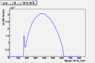
3 SIGNAL EVENT SELECTION

After event generation using CompHEP, PYTHIA and the CompHEP-PYTHIA interface packages with the Les Houches Accord implemented[261] an approximate response of an ILC detector was simulated by means of SIMDET_-v4 [262].

The most important background consists of  $t\bar{t}+(\gamma)$ events, where photons from initial state radiation (ISR) are not detected. The number of events expected for both energies are given in Table 2. They exceed substantially the number of signal events (see Table 1) for the chosen value for the parameter $M/\sqrt{c_{t}}$. The next significant background to consider is $e^{+}e^{-}\to t\bar{t}+\nu\bar{\nu}$, with the same signature as for the signal. The corresponding event numbers also given in Table 2 are comparable to the signal event rates for not too small $M/\sqrt{c_{t}}$ values. An invariant mass cut of e.g. $M_{\nu\bar{\nu}}<$ 80 GeV, i.e. a cut on the event missing mass, removes most of these events.

$background$	$\sqrt{s}=0.5\leavevmode\nobreak\ TeV$	$\sqrt{s}=1\leavevmode\nobreak\ TeV$
$t\bar{t}(\gamma)$	$276675$	$200310$
$t\bar{t}\nu\bar{\nu}$	$75$	$930$

Table 2: Background events at $\sqrt{s}=0.5$ and 1 TeV for an integrated luminosity of 0.5, respectively, 1 ab^-1.

To discriminate signal and a very large background we use a multivariate technique based on likelihood method. 18 kinematics variables, such as missing energy, invariant masses of various jet combinations etc. were combined into a global discriminant variable $P_{P}$, designed to give a measure of the ’Paraphoton-likeness’ of any particular event. As it should be the background events are preferentially distributed at low $P_{P}$ values while for signal events $P_{P}$ is concentrated close to unity. By choosing optimal values of cuts for the discriminant $P_{P}$ one gets the signal selection efficiency of 49% (76%) at $\sqrt{s}$ = 0.5 (1) TeV, while only 9% of background events survive. At $\sqrt{s}$ = 0.5 TeV, S/$\sqrt{B}$ = 11.96 for $M/\sqrt{c_{t}}=0.2$ TeV, while S/$\sqrt{B}$ = 162.6 at 1 TeV, i.e. the probability of measuring the total event rates as a result of a background fluctuation is $0.5\cdot 10^{-12}$ and $<10^{-15}$ at 0.5, respectively, 1 TeV, using Gaussian sampling of uncertainties. In this way, an almost background-free signal event sample can be extracted for further measurements at 1 TeV. The situation is much less convenient at 0.5 TeV.

4 DISCUSSION OF THE RESULTS

If an excess of signal events over the SM background is established, limits on the inverse coupling parameter $M/\sqrt{c_{t}}$ accessible for a significance of $S/\sqrt{B}=5$ can be derived being sufficient for the paraphoton discovery. The numbers of surviving $\gamma^{\prime}$ events for 5$\sigma$ discovery at 0.5 and 1 TeV energies and an integrated luminosity of 0.5 and 1.0 ab^-1 can be converted into limits for $M/\sqrt{c_{t}}$. These limits are found to be of 0.33 and 0.61 TeV for 0.5 and 1 TeV cases respectively. The value $M/\sqrt{c_{t}}=0.61$ TeV, is expected to be the most stringent limit accessible at the ILC.

The signal-to-background ratio, $S/B$, is about 1.79 at 1 TeV, sufficiently large to understand a spin assignment of the radiated massless particle. In order to demonstrate the spin-1 nature of the $\gamma^{\prime}$, we follow studies performed to establish the vector nature of the gluon in 3-jet $e^{+}e^{-}$ annihilation events at PETRA [263, 264, 265, 266] and LEP [267, 268, 269] energies, based on predictions that a spin-$\frac{1}{2}$ quark radiates the spin-1 gluon. The analysis of the Ellis-Karliner angle [270] distribution and the polar angle distribution of the normal to the reaction plane at 1 TeV clearly shows that spin-1 assignment for the paraphoton is highly favored over spin 0.

5 CONCLUSIONS

Some realistic extensions of the Standard Model suggest the existence of a new massless neutral gauge boson, denoted as the paraphoton $\gamma^{\prime}$ in this study. This particle is similar to the ordinary photon, but the interactions of the $\gamma^{\prime}$ are very distinct: couplings to SM fermions are proportional to fermion masses and therefore strongest to the top quark, and grow with the $\gamma^{\prime}$ momentum. Hence, the paraphoton radiation off the top at the ILC is studied as the most promising process for the paraphoton observation. Only the all-hadronic top decay mode was selected to ensure a high signal-to-background ratio and to avoid complications due to final state neutrinos in leptonic W decays. A multivariate search strategy was used to better separate the signal from backgrounds. Allowing for a 5$\sigma$ paraphoton discovery significance, $e^{+}e^{-}$ collisions at 1 TeV allow to bound the $\gamma^{\prime}$-top quark inverse coupling to $M/\sqrt{c_{t}}\stackrel{{\scriptstyle<}}{{{}_{\sim}}}0.61$ TeV, which is expected to be the most stringent limit accessible at the next generation colliders. For the sake of demonstration two angular variables, the Ellis-Karliner angle and the polar angle of the normal to the $t\leavevmode\nobreak\ \bar{t}\leavevmode\nobreak\ \gamma^{\prime}$ plane as a function of a thrust cut-off, were studied to establish the vector nature of the $\gamma^{\prime}$. Both angular distributions are in accord with the spin-1 assignment of the paraphoton and inconsistent with e.g. a scalar hypothesis.

ACKNOWLEDGEMENTS

The work of E.B. and V.B. is partly supported by the grant NS.1685.2003.2 of the Russian Ministry of Education and Science. V.B. acknowledges support of the grant of ”Dynasty” Foundation. E.B. and V.B. are grateful to DESY and Fermilab for the kind hospitality. We thank the organizers of the Les Houches Workshop for a productive scientific atmosphere. Especially we would like to thank Bogdan Dobrescu for many valuable discussions.

Part 16 High $p^{T}$ Hadronic Top Quark Identification

G. Brooijmans

1 INTRODUCTION

At the LHC, top quarks, $W$ and $Z$ bosons are relatively light and can be produced with very high transverse momenta with respect to their masses. In the case of hadronic decays, the quarks can be so close together in the detector that they are in principle reconstructed as a single jet. This is illustrated in Figure 1, which shows generator-level distributions of angular distance between the b quark and $W$ boson, and quarks from $W$ boson decays in $t\bar{t}$ events. Here $dR=\sqrt{(\Delta\phi)^{2}+(\Delta\eta)^{2}}$ with $\phi$ the azimuthal angle and $\eta$ the rapidity. For top quark transverse momenta larger than about 200 GeV, the distance between the decay products is often smaller than twice the typical jet radius. These events were generated using PYTHIA [271] and no top polarization effects are included. Such effects are very model dependent and therefore beyond the scope of this generic study.

Figure 1: Angular distances between decay products in top quark decays as a function of top quark transverse momentum: (a) between the b quark and $W$ boson, and (b) between quarks from $W$ boson decays.

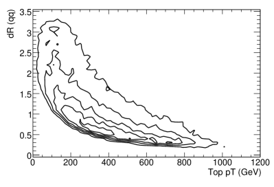
Identifying top quarks at high transverse momentum with high efficiency is of particular interest in searches for new physics. In addition to a number of recent theoretical models specifically proposing the existence of high mass resonances decaying dominantly to top quarks (see for example [142, 244, 133, 176, 104]), the large top quark mass suggests it might be closely linked to forms of new physics that would manifest themselves at very high energies. It is therefore quite probable that new heavy objects decay to top quarks at least some fraction of the time, if not exclusively.

2 DATASETS AND TOOLS

The datasets used in this study are a) sequential standard model $Z^{\prime}$-bosons of mass 2 and 3 TeV decaying to top-antitop pairs for signal, and b) multijet events with transverse momenta ranging from 300 to 2200 GeV for the background. For the signal events, one of the top quarks is forced to decay hadronically, and the other semileptonically. The events were all generated using PYTHIA, passed through the full ATLAS detector simulation and reconstructed using the ATLAS reconstruction program.

The jet mass, which is the invariant mass of all the jet’s constituents (typically calorimeter cells or towers), and “YSplitter” [214], which determines the scales at which jets can be resolved into two or more subjets are used as discriminating variables. Top “monojets” are selected in the signal samples by selecting events in which only one jet with $p_{T}>20$ GeV has $dR<1.0$ from the closest top quark and $dR<2.0$ from the hadronically decaying $W$ boson. For these jets, Figure 2 shows the distribution of jet mass as a function of jet transverse momentum, and the scales at which the jet splits up into two and three jets.

Figure 2: (a) Jet mass as a function of transverse momentum for jets passing the top monojet selection: jets from the M = 2 (3) TeV $Z^{\prime}$ sample in blue (red). (b) and (c) Solid (dashed): scales at which the top monojet splits into two and three jets respectively for events in the $M_{Z^{\prime}}=2(3)$ TeV samples.

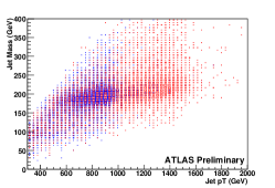
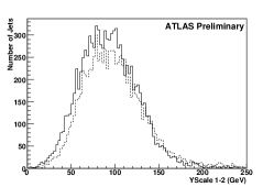
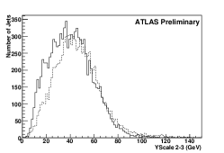
The distributions have only limited dependence on the jet transverse momentum distribution and are therefore well suited to the identification of top monojets over a wide spectrum. The splitting scales into two and three jets cluster around half the top quark mass and half the $W$-boson mass respectively as expected. The same distributions are shown for the background samples in Figure 3.

Figure 3: (a) Jet mass as a function of transverse momentum, (b) and (c) scales at which the jet splits into two and three jets respectively for events in the background samples.

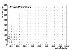
3 QUANTITATIVE ANALYSIS

In principle, with this number of variables a multivariate tool like an artificial neural network might yield optimal results in terms of high/low efficiency for signal/background. For the sake of clarity however this study is based on simple two-dimensional cuts, keeping in mind that the use of multivariate tools typically leads to a factor of approximately 1.5 improvement in the signal over background ratio.

Cuts are applied on

1. Jet mass ($>170$ GeV),

2. jet mass as a function of jet transverse momentum,

3. YScale 1-2 (split from one to two jets) as a function of YScale 2-3 (split from two to three jets),

4. YScale 2-3 as a function of YScale 3-4,

5. YScale 1-2 as a function of jet mass,

6. YScale 2-3 as a function of jet mass, and

7. YScale 3-4 as a function of jet mass (two cuts).

As an illustration, three of these (2, 4 and 7) are shown in Figure 4.

Figure 4: Cuts applied on (a) jet mass as a function of jet transverse momentum (events are required to lie below the line), (b) $YScale_{23}$ as a function of $YScale_{34}$ (events are required to lie above the line), and (c) $YScale_{34}$ as a function of jet mass (events are required to lie above the line). In each plot, the background is in blue and the signal in red.

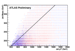
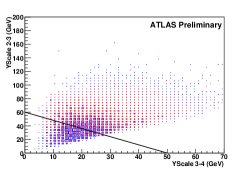
The resulting efficiencies for signal and background events are shown in Figure 5. For the background the efficiency plateaus at about 10% starting at jet transverse momenta of 1300 GeV, where the signal efficiency reaches 60%. The ratio of signal over background efficiency increases for smaller jet transverse momenta. A more detailed description of this analysis is available in [272].

Figure 5: Selection efficiency as a function of transverse momentum for top monojets (solid, black) and jets in the background samples (blue, dashed).

4 CONCLUSIONS

In this analysis, the measured jet mass and jet splitting scales have been used to distinguish high transverse momentum “top monojets” from jets originating from light quarks. The combination of algorithms allows for good separation of signal and background, with the ratio of selection efficiencies for signal and background evolving from approximately 30 for jets with $p_{T}=$ 600 GeV to 10 for 1000 GeV and 7 for 1500 GeV. Further work using subjets and tracking information is underway.

ACKNOWLEDGEMENTS

This work has been performed within the ATLAS Collaboration, and we thank collaboration members for helpful discussions. We have also made use of the physics analysis framework and tools which are the result of collaboration-wide efforts.

blabla

A Les Houches Interface

Part 17 A Les Houches Interface for BSM Generators

J. Alwall, E. Boos, L. Dudko, M. Gigg, M. Herquet, A. Pukhov, P. Richardson, A. Sherstnev and P. Skands

1 INTRODUCTION

The simulation of interactions at the LHC is characterized by the use of many different programs specializing in different stages of the calculation, such as matrix-element-level event generation, decay of resonances, parton showering, hadronization, and underlying event simulation. The communication of simulation parameters between those stages can be complicated and program-specific. For supersymmetric models, this situation has been greatly improved by the introduction of the SUSY Les Houches Accord [273] (SLHA) and its upcoming extension [274]. For general models however, there is still no corresponding standard. In this note, we suggest an addition to the SLHA to allow for the specification of the quantum numbers, masses, and decays of arbitrary new states, thus generalizing the accord beyond its original supersymmetry-specific scope. We also make a proposal for how to include these model parameter files into Les Houches Accord event files [275] (LHEF) in a standardized way. This both reduces the number of files that need to be passed around and minimizes the possibility for error by keeping all relevant model information together with the actual events.

2 DEFINITION OF THE INTERFACE

The concrete proposal consists of the following three points:

1. Introduce new SLHA-like blocks QNUMBERS (for “quantum numbers”) with the format:

   BLOCK QNUMBERS 7654321 # balleron
       1     0  # 3 times electric charge
       2     1  # number of spin states (2S+1)
       3     1  # colour rep (1: singlet, 3: triplet, 8: octet)
       4     0  # Particle/Antiparticle distinction (0=own anti)
   

   where this example pertains to a fictitious neutral spin-0 color-singlet self-conjugate particle to which we assign “PDG” code 7654321 and the name “balleron”. That is, the BLOCK declaration should define a PDG code and, optionally, a human readable name after the # character (if no name is given, the PDG code may be used). We advise to choose PDG numbers in excess of 3 million for new states, to minimize the possibility of conflict with already agreed-upon numbers [85]. The entries so far defined are: 1: the electric charge times 3 (so that most particles will have integer values, but real numbers should also be accepted); 2: the particle’s number of spin states: $2S+1$; 3: the colour representation of the particle, e.g., 1 for a singlet, 3 (-3) for a triplet (antitriplet), 8 for an octet, etc.; 4: particle/antiparticle distincition, should be 0 (zero) if the particle is its own antiparticle, or 1 otherwise.

2. Use the existing SLHA blocks MASS and DECAY [273] to define particle masses and decay tables. If the model in question is a SUSY model, a full SLHA spectrum [273] can also be included. We propose that the reader should “turn on” SUSY whenever the SLHA SUSY model definition block MODSEL is present.

3. Include the information from points 1 and 2 enclosed within the subtags <slha> </slha> in the <header> part of Les Houches event files [275].

3 IMPLEMENTATIONS

For the purpose of this contribution, the above proposal was tested explicitly by interfacing MadGraph/MadEvent with Pythia. Below we summarize the main aspects of these implementations.

3.1 MadGraph/MadEvent implementation

Starting from version 4 [35], the multi-purpose MadGraph/MadEvent parton-level event generator by default includes a detailed summary of all simulation parameters in the output LHEF [275] parton-level event file. From version 4.1.47, this information is stored in the XML <header> section. For the interface considered here, the relevant part of this section is a copy of the so-called param_card.dat MG/ME input file.

The MG/ME param_card.dat uses an extension of the SUSY Les Houches Accord [273, 274] for model parameters in all implemented models. In particular, it always includes the SMINPUTS, MASS, and DECAY blocks. This file is used by MadGraph/MadEvent as an input for cross section computations and event generation but is not modified by the program. The file is instead assumed to be created by an external “Model Calculator”. Such calculators are currently available on the web for the SM, MSSM and 2HDM models. Starting from the parameters in the Lagrangian (primary parameters), they calculate all needed secondary parameters (such as masses, decay widths, and auxiliary parameters). Note that widths and branching ratios can also be evaluated in an intermediate step by MG/ME itself or by external tools like DECAY or BRIDGE [84].

In previous versions of MadGraph/MadEvent, the param_card.dat file did not contain information regarding the particle content of the physical model considered. This information is stored in the particle.dat file filled by model writers during the model creation. Starting from version 4.1.43, the template for inclusion of user defined models (called USRMOD) in MadGraph/MadEvent automatically generates the QNUMBERS blocks described above from the information contained in the particle.dat file. These blocks are then included in the default param_card.dat for the new model (and from there are copied into the LHEF output), such that no extra intervention is required to pass them to parton shower programs after parton-level event production. The script only outputs information for particles which have PDG numbers not identified as standard SM or MSSM particles, since those are assumed to be defined in the parton shower generators.

Note that in the current version, the spin, color and particle/antiparticle information is automatically extracted, but not the electric charge, which is set to zero by default. This is due to the fact that, in MadGraph/MadEvent, the electric charge does not appear in the list of particle properties and is only defined through the value of the coupling to the photon. This issue will be addressed in future versions of USRMOD, but can currently be circumvented by fixing the electric charge information by hand at the end of the model implementation process.

3.2 Pythia implementation

The following capabilities are implemented in Pythia 6.414 [75] and subsequent versions.

Already for some time it has been possible to use the QNUMBERS blocks described above to define new particles in Pythia via its SLHA interface [276]. What is new is that, when reading an LHEF event file, Pythia now automatically searches for QNUMBERS blocks in the header part of the LHEF file, updating its internal particle data tables accordingly. It then proceeds to search for MASS and DECAY tables, and finally looks for other SLHA blocks contained in the header. If the SUSY model definition block MODSEL is found, SUSY is automatically switched on and the remaining SLHA blocks are read, without the user having to intervene. The read-in of LHEF files containing general BSM states, masses, and decay tables, should therefore now be relatively “ plug-and-play”.

A note on decay tables: only 2- and 3-body decays can currently be handled consistently. They are then generated with flat phase space, according to the branching ratios input via the DECAY tables. The colour flow algorithms have been substantially generalized, but if too many coloured particles are involved (e.g., an octet decaying to three octets) Pythia will still not be able to guess which colour flow to use, leading to errors. Please also read the warnings in the section on decay tables in the SLHA report [273] concerning the dangers of double counting partial widths and obliterating resonance shapes. To get around the restriction to flat phase space, either 1) use Pythia’s internal resonance decays whenever possible (e.g., do not read in decay tables for particles for which Pythia’s internal treatment is not desired modified), 2) perform the decays externally, before the event is handed to Pythia (e.g., with MadGraph/Bridge [84] or CalcHEP [277]), or 3) do a post facto re-weighting of the generated events, based on the kinematics of the particle decays stored in the event record.

The interfaces can of course still also be used stand-alone, independently of LHEF. The user must then manually open a spectrum file containing QNUMBERS and MASS information and give Pythia the logical unit number in IMSS(21). New states can then be read in via either of the calls
           CALL PYSLHA(0,KF,IFAIL)    ! look for QNUMBERS for PDG = KF
           CALL PYSLHA(0,0,IFAIL)     ! read in all QNUMBERS
and MASS information can be read by
           CALL PYSLHA(5,KF,IFAIL)    ! look for MASS entry for PDG = KF
           CALL PYSLHA(5,0,IFAIL)     ! read in all MASS entries
where IFAIL is a standard return code, which is zero if everything went fine. (For read-in of a complete SLHA SUSY spectrum file, these direct calls should not be used, instead set IMSS(1)=11 before the call to PYINIT.) For stand-alone decay table read-in, the unit number of the SLHA decay table file should be given in IMSS(22), and the corresponding read-in calls are
           CALL PYSLHA(2,KF,IFAIL)    ! look for DECAY table for PDG = KF
           CALL PYSLHA(2,0,IFAIL)     ! read in all DECAY tables

4 CONCLUSIONS AND OUTLOOK

We have proposed a simple file-based interface between parton- and event-level generators focusing on the particular problems encountered in the simulation of beyond-the-standard-model collider physics. To deal with general BSM models, we add a new block QNUMBERS to the SLHA structure, which defines the SM quantum numbers of new states for use in subsequent resonance decay, parton showering, and hadronization programs. We also integrate the SLHA file into the existing LHEF format to minimize the number of separate files needed. The proposal has been tested explicitly by implementations in the MadGraph/MadEvent and Pythia6 Monte Carlo event generators.

In the near future, also the Herwig++ [11] and Pythia8 [278] generators will be extended to automatically read in SLHA spectra from LHEF headers. Likewise, forthcoming versions of the CalcHEP [34] and CompHEP [258] parton-level generators will include write-out of this information in their LHEF output, including also the QNUMBERS extension.

In the longer term, with the XML format emerging as the de facto standard for file-based interfaces, we note that it could be worth investigating the merits of formulating an XML-SLHA scheme, that is, transforming the current ASCII SLHA format conventions into a native XML form that could be parsed with standard XML packages. A concrete first realization of such a strategy is HepML [279] which aims to unify the description of generator information in the form of standard XML schemes, in which an XML-SLHA scheme would form a natural part. The first release of the public HepML library has been implemented into CompHEP version 4.5, including also HepML headers in the LHEF output.

ACKNOWLEDGEMENTS

The proposal and implementations contained herein originated at the workshop “Physics at TeV Colliders”, Les Houches, France, 2007. This work has been partially supported by Fermi Research Alliance, LLC, under Contract No. DE-AC02-07CH11359 with the United States Department of Energy. The work of MH was supported by the Institut Interuniversitaire des Sciences Nucléaires and by the Belgian Federal Office for Scientific, Technical and Cultural Affairs through the Interuniversity Attraction Pole P6/11. The HepML project is supported by the RFBR-07-07-00365 grant. The work of JA was was supported by the Swedish Research Council.

References

- [1] B.W. Lee, C. Quigg, and H.B. Thacker, Phys. Rev. D16 (1977) 1519.
- [2] T. Appelquist, H.-C. Cheng, and B.A. Dobrescu, Phys. Rev. D64 (2001) 035002, [hep-ph/0012100].
- [3] N. Arkani-Hamed, S. Dimopoulos, and G.R. Dvali, Phys. Lett. B429 (1998) 263–272, [hep-ph/9803315].
- [4] N. Arkani-Hamed, S. Dimopoulos, and G.R. Dvali, Phys. Rev. D59 (1999) 086004, [hep-ph/9807344].
- [5] H.-C. Cheng, K.T. Matchev, and M. Schmaltz, Phys. Rev. D66 (2002) 056006, [hep-ph/0205314].
- [6] C. Lin, FERMILAB-THESIS-2005-69.
- [7] G. Servant and T.M.P. Tait, Nucl. Phys. B650 (2003) 391–419, [hep-ph/0206071].
- [8] D. Acosta et. al. (CMS Collaboration), CERN/LHCC 2006-001, CMS TDR 8.1 (2006).
- [9] R. Alemany-Fernandez, M. Kazana, P. Ribeiro, and J. Varela, CMS analysis note, CMS CR-2006/008.
- [10] H.-C. Cheng, K.T. Matchev and M. Schmaltz, Phys. Rev. D66 (2002) 036005, [hep-ph/0204342].
- [11] M. Bahr et. al., arXiv:0711.3137 [hep-ph].
- [12] M. Gigg and P. Richardson, Eur. Phys. J. C51 (2007) 989–1008, [hep-ph/0703199].
- [13] M. Muhlleitner, A. Djouadi and Y. Mambrini, Comput. Phys. Commun. 168 (2005) 46–70, [hep-ph/0311167].
- [14] J.M. Smillie and B.R. Webber, JHEP 10 (2005) 069, [hep-ph/0507170].
- [15] C. Csaki, C. Grojean, H. Murayama, L. Pilo and J. Terning, Phys. Rev. D69 (2004) 055006, [hep-ph/0305237].
- [16] K. Agashe, A. Delgado, M.J. May and R. Sundrum, JHEP 08 (2003) 050, [hep-ph/0308036].
- [17] C. Csaki, C. Grojean, L. Pilo and J. Terning, Phys. Rev. Lett. 92 (2004) 101802, [hep-ph/0308038].
- [18] J.M. Maldacena, Adv. Theor. Math. Phys. 2 (1998) 231–252, [hep-th/9711200].
- [19] B. Holdom, Phys. Rev. D24 (1981) 1441.
- [20] B. Holdom, Phys. Lett. B150 (1985) 301.
- [21] K. Yamawaki, M. Bando, and K.-i. Matumoto, Phys. Rev. Lett. 56 (1986) 1335.
- [22] T. Appelquist, D. Karabali and L.C.R. Wijewardhana, Phys. Rev. Lett. 57 (1986) 957.
- [23] T. Appelquist and L.C.R. Wijewardhana, Phys. Rev. D35 (1987) 774.
- [24] T. Appelquist and L.C.R. Wijewardhana, Phys. Rev. D36 (1987) 568.
- [25] R.S. Chivukula, D.A. Dicus and H.-J. He, Phys. Lett. B525 (2002) 175–182, [hep-ph/0111016].
- [26] R.S. Chivukula, E.H. Simmons, H.-J. He, M. Kurachi and M. Tanabashi, Phys. Rev. D71 (2005) 035007, [hep-ph/0410154].
- [27] G. Cacciapaglia, C. Csaki, C. Grojean and J. Terning, Phys. Rev. D71 (2005) 035015, [hep-ph/0409126].
- [28] G. Cacciapaglia, C. Csaki, C. Grojean, M. Reece and J. Terning, Phys. Rev. D72 (2005) 095018, [hep-ph/0505001].
- [29] R. Foadi, S. Gopalakrishna and C. Schmidt, Phys. Lett. B606 (2005) 157–163, [hep-ph/0409266].
- [30] R.S. Chivukula, E.H. Simmons, H.-J. He, M. Kurachi and M. Tanabashi, Phys. Rev. D72 (2005) 015008, [hep-ph/0504114].
- [31] R.S. Chivukula, E.H. Simmons, H.-J. He, M. Kurachi and M. Tanabashi, Phys. Rev. D72 (2005) 075012, [hep-ph/0508147].
- [32] R.S. Chivukula et. al., Phys. Rev. D74 (2006) 075011, [hep-ph/0607124].
- [33] R. Casalbuoni, S. De Curtis, D. Dominici and R. Gatto, Phys. Lett. B155 (1985) 95.
- [34] A. Pukhov, hep-ph/0412191.
- [35] J. Alwall et. al., JHEP 09 (2007) 028, [arXiv:0706.2334 [hep-ph]].
- [36] H.-J. He et. al., arXiv:0708.2588 [hep-ph].
- [37] The ATLAS collaboration, Technical Design Report, Vol. 2, CERN-LHCC-99-15 (1999).
- [38] J. Bagger et. al., Phys. Rev. D52 (1995) 3878–3889, [hep-ph/9504426].
- [39] H.-J. He, Y.-P. Kuang, C.P. Yuan and B. Zhang, Phys. Lett. B554 (2003) 64–72, [hep-ph/0211229].
- [40] B. Zhang, Y.-P. Kuang, H.-J. He and C.P. Yuan, Phys. Rev. D67 (2003) 114024, [hep-ph/0303048].
- [41] A. Birkedal, K. Matchev and M. Perelstein, Phys. Rev. Lett. 94 (2005) 191803, [hep-ph/0412278].
- [42] H.-J. He et. al., work in preparation (2008).
- [43] S. Weinberg, Phys. Rev. D19 (1979) 1277–1280.
- [44] L. Susskind, Phys. Rev. D20 (1979) 2619–2625.
- [45] K. Yamawaki, M. Bando and K.-i. Matumoto, Phys. Rev. Lett. 56 (1986) 1335.
- [46] T. Akiba and T. Yanagida, Phys. Lett. B169 (1986) 432.
- [47] E. Eichten and K. Lane, Phys. Lett. B90 (1980) 125–130.
- [48] K. Lane, hep-ph/0202255.
- [49] C.T. Hill and E.H. Simmons, Physics Reports 381 (2003) 235–402, [hep-ph/0203079].
- [50] K. Lane and E. Eichten, Phys. Lett. B222 (1989) 274.
- [51] E. Eichten and K. Lane, Phys. Lett. B388 (1996) 803–807, [hep-ph/9607213].
- [52] E. Eichten, K. Lane and J. Womersley, Phys. Lett. B405 (1997) 305–311, [hep-ph/9704455].
- [53] E. Eichten, I. Hinchliffe, K. Lane and C. Quigg, Rev. Mod. Phys. 56 (1984) 579–707.
- [54] T. Appelquist and R. Shrock, Phys. Lett. B548 (2002) 204–214, [hep-ph/0204141].
- [55] T. Appelquist, M. Piai and R. Shrock, Phys. Rev. D69 (2004) 015002, [hep-ph/0308061].
- [56] K. Lane, hep-ph/9401324.
- [57] K. Lane, hep-ph/9409304.
- [58] M.E. Peskin and T. Takeuchi, Phys. Rev. Lett. 65 (1990) 964–967.
- [59] M. Golden and L. Randall, Nucl. Phys. B361 (1991) 3–23.
- [60] B. Holdom and J. Terning, Phys. Lett. B247 (1990) 88–92.
- [61] G. Altarelli, R. Barbieri and S. Jadach, Nucl. Phys. B369 (1992) 3–32.
- [62] T. Appelquist and F. Sannino, Phys. Rev. D59 (1999) 067702, [hep-ph/9806409].
- [63] M. Knecht and E. de Rafael, Phys. Lett. B424 (1998) 335–342, [hep-ph/9712457].
- [64] J. Hirn and V. Sanz, Phys. Rev. Lett. 97 (2006) 121803, [hep-ph/0606086].
- [65] J. Hirn and V. Sanz, hep-ph/0612239.
- [66] E. Eichten and K. Lane, arXiv:0706.2339 [hep-ph].
- [67] K. Lane, Phys. Rev. D60 (1999) 075007, [hep-ph/9903369].
- [68] K. Lane and S. Mrenna, Phys. Rev. D67 (2003) 115011, [hep-ph/0210299].
- [69] C.T. Hill, Phys. Lett. B345 (1995) 483–489, [hep-ph/9411426].
- [70] P. Kreuzer, Acta Phys. Polon. B38 (2007) 459–468.
- [71] “PGS – Pretty Good Simulator”, http://www.physics.ucdavis.edu/ conway/research/software/pgs/pgs4-general.html
- [72] R.S. Chivukula, E.H. Simmons, H.-J. He, M. Kurachi and M. Tanabashi, Phys. Rev. D71 (2005) 115001, [hep-ph/0502162].
- [73] E. Richter-Was, D. Froidevaux and L. Poggioli, “AtlFast,” ATLAS note, ATL-PHYS-98-131, http://www.hep.ucl.ac.uk/atlas/atlfast/UserGuide.html, 1998.
- [74] G. Azuelos, J. Ferland, K. Lane and A. Martin, “Search for low-scale technicolor in atlas,” ATLAS note, ATL-PHYS-CONF-2008-003, 2008.
- [75] T. Sjostrand, S. Mrenna and P. Skands, JHEP 05 (2006) 026, [hep-ph/0603175].
- [76] F. Maltoni and T. Stelzer, JHEP 02 (2003) 027, [hep-ph/0208156].
- [77] M.L. Mangano, M. Moretti, F. Piccinini, R. Pittau and A.D. Polosa, JHEP 07 (2003) 001, [hep-ph/0206293].
- [78] K. Black, “Searches for technicolor in the trilepton final state,” ATLAS note, ATL-PHYS-CONF-2008-004, 2008.
- [79] T. Bose, CMS note, CMS CR-2008/004.
- [80] S.S. Gubser, I.R. Klebanov and A.M. Polyakov, Phys. Lett. B428 (1998) 105–114, [hep-th/9802109].
- [81] E. Witten, Adv. Theor. Math. Phys. 2 (1998) 253–291, [hep-th/9802150].
- [82] K. Agashe, C. Csaki, C. Grojean and M. Reece, JHEP 12 (2007) 003, [arXiv:0704.1821 [hep-ph]].
- [83] R. Sundrum and S.D.H. Hsu, Nucl. Phys. B391 (1993) 127–146, [hep-ph/9206225].
- [84] P. Meade and M. Reece, hep-ph/0703031.
- [85] W. M. Yao et. al., Particle Data Group Collaboration J. Phys. G33 (2006) 1–1232.
- [86] T. Aaltonen et. al. (CDF Collaboration), Phys. Rev. Lett. 99 (2007) 171802, [arXiv:0707.2524 [hep-ex]].
- [87] A. Abulencia et. al. (CDF Collaboration), Phys. Rev. D75 (2007) 091101, [hep-ex/0611022].
- [88] K.-m. Cheung, Phys. Lett. B517 (2001) 167–176, [hep-ph/0106251].
- [89] V. M. Abazov et. al. (DØ Collaboration), Phys. Rev. D71 (2005) 091108, [hep-ex/0503048].
- [90] A. Abulencia et. al. (CDF Collaboration), Phys. Rev. Lett. 98 (2007) 161801, [hep-ex/0702027].
- [91] CDF Collaboration, CDF note 8452 (2007).
- [92] J. Hirn, A. Martin and V. Sanz, arXiv:0712.3783 [hep-ph].
- [93] J. Hirn, A. Martin and V. Sanz, to appear.
- [94] G. Azuelos et al,. Proceedings, Workshop, Les Houches, France, 2007. To appear.
- [95] K.-m. Cheung and G.L. Landsberg, Phys. Rev. D62 (2000) 076003, [hep-ph/9909218].
- [96] B. Abbott et. al. (DØ Collaboration), Phys. Rev. Lett. 86 (2001) 1156–1161, [hep-ex/0008065].
- [97] V. M. Abazov et. al. (DØ Collaboration), Phys. Rev. Lett. 95 (2005) 161602, [hep-ex/0506063].
- [98] M.S. Carena, A. Daleo, B.A. Dobrescu and T.M.P. Tait, Phys. Rev. D70 (2004) 093009, [hep-ph/0408098].
- [99] C. Anastasiou, L.J. Dixon, K. Melnikov and F. Petriello, Phys. Rev. D69 (2004) 094008, [hep-ph/0312266].
- [100] F. Petriello and S. Quackenbush, arXiv:0801.4389 [hep-ph].
- [101] S. Weinberg, Phys. Rev. Lett. 29 (1972) 1698–1701.
- [102] H. Georgi and A. Pais, Phys. Rev. D12 (1975) 508.
- [103] D.B. Kaplan and H. Georgi, Phys. Lett. B136 (1984) 183.
- [104] R. Contino and G. Servant, arXiv:0801.1679 [hep-ph].
- [105] T. Bose and M. Narain, CMS note, CMS CR-2008/005.
- [106] P. Sikivie, L. Susskind, M.B. Voloshin and V.I. Zakharov, Nucl. Phys. B173 (1980) 189.
- [107] K. Agashe, R. Contino, L. Da Rold and A. Pomarol, Phys. Lett. B641 (2006) 62–66, [hep-ph/0605341].
- [108] C. Dennis, M. Karagoz Unel, G. Servant and J. Tseng, hep-ph/0701158.
- [109] W. Skiba and D. Tucker-Smith, Phys. Rev. D75 (2007) 115010, [hep-ph/0701247].
- [110] R. Bonciani, S. Catani, M.L. Mangano and P. Nason, Nucl. Phys. B529 (1998) 424–450, [hep-ph/9801375].
- [111] The ATLAS collaboration, Technical Design Report, Vol. 1, CERN-LHCC-99-014 (1999) Section 3.3.
- [112] T. Stelzer and W.F. Long, Comput. Phys. Commun. 81 (1994) 357–371, [hep-ph/9401258].
- [113] F. Paige and S. Protopopescu, in Physics of the SSC, Snowmass, Colorado, edited by R. Donaldson and J. Marx”, 1986.
- [114] J. Alwall et. al., Eur. Phys. J. C53 (2008) 473–500, [arXiv:0706.2569 [hep-ph]].
- [115] M.L. Mangano, M. Moretti, F. Piccinini and M. Treccani, JHEP 01 (2007) 013, [hep-ph/0611129].
- [116] S. Hoeche et. al., hep-ph/0602031.
- [117] S. Dimopoulos and H. Georgi, Nucl. Phys. B193 (1981) 150.
- [118] S. Weinberg, Phys. Rev. D13 (1976) 974–996.
- [119] C.T. Hill, Phys. Rev. D24 (1981) 691.
- [120] C.T. Hill, Phys. Lett. B266 (1991) 419–424.
- [121] R.S. Chivukula, B.A. Dobrescu, H. Georgi and C.T. Hill, Phys. Rev. D59 (1999) 075003, [hep-ph/9809470].
- [122] B.A. Dobrescu and C.T. Hill, Phys. Rev. Lett. 81 (1998) 2634–2637, [hep-ph/9712319].
- [123] D.B. Kaplan, H. Georgi and S. Dimopoulos, Phys. Lett. B136 (1984) 187.
- [124] N. Arkani-Hamed, A.G. Cohen and H. Georgi, Phys. Lett. B513 (2001) 232–240, [hep-ph/0105239].
- [125] N. Arkani-Hamed, A.G. Cohen, E. Katz and A. E. Nelson, JHEP 07 (2002) 034, [hep-ph/0206021].
- [126] M. Schmaltz and D. Tucker-Smith, Ann. Rev. Nucl. Part. Sci. 55 (2005) 229–270, [hep-ph/0502182].
- [127] N. Arkani-Hamed, S. Dimopoulos and G.R. Dvali, Phys. Lett. B429 (1998) 263–272, [hep-ph/9803315].
- [128] L. Randall and R. Sundrum, Phys. Rev. Lett. 83 (1999) 3370–3373, [hep-ph/9905221].
- [129] J.L. Hewett and T.G. Rizzo, Phys. Rept. 183 (1989) 193.
- [130] M. Cvetic and P. Langacker, Phys. Rev. D54 (1996) 3570–3579, [hep-ph/9511378].
- [131] K. Lane, Phys. Rev. D52 (1995) 1546–1555, [hep-ph/9501260].
- [132] V. Barger, T. Han and D.G.E. Walker, hep-ph/0612016.
- [133] A.L. Fitzpatrick, J. Kaplan, L. Randall and L.-T. Wang, JHEP 09 (2007) 013, [hep-ph/0701150].
- [134] B. Lillie, L. Randall and L.-T. Wang, JHEP 09 (2007) 074, [hep-ph/0701166].
- [135] G. Shiu, B. Underwood, K. M. Zurek and D.G.E. Walker, arXiv:0705.4097 [hep-ph].
- [136] U. Baur and L.H. Orr, Phys. Rev. D76 (2007) 094012, [arXiv:0707.2066 [hep-ph]].
- [137] K. Agashe et. al., Phys. Rev. D76 (2007) 115015, [arXiv:0709.0007 [hep-ph]].
- [138] R.N. Mohapatra, N. Okada and H.-B. Yu, Phys. Rev. D77 (2008) 011701, [arXiv:0709.1486 [hep-ph]].
- [139] M. Gerbush, T.J. Khoo, D.J. Phalen, A. Pierce and D. Tucker-Smith, arXiv:0710.3133 [hep-ph].
- [140] L. Cavicchia, R. Franceschini and V.S. Rychkov, arXiv:0710.5750 [hep-ph].
- [141] R. Frederix and F. Maltoni, arXiv:0712.2355 [hep-ph].
- [142] K. Agashe, A. Belyaev, T. Krupovnickas, G. Perez and J. Virzi, hep-ph/0612015.
- [143] B. Abbott et. al. (DØ Collaboration), Phys. Rev. D58 (1998) 052001, [hep-ex/9801025].
- [144] F. Abe et. al. (CDF Collaboration), Phys. Rev. Lett. 80 (1998) 2767–2772, [hep-ex/9801014].
- [145] V. D. Barger, J. Ohnemus and R.J.N. Phillips, Int. J. Mod. Phys. A4 (1989) 617.
- [146] M. Arai, N. Okada, K. Smolek and V. Simak, Phys. Rev. D70 (2004) 115015, [hep-ph/0409273].
- [147] A. Ball, M. Della Negra, L. Foa and A. Petrilli, CMS Physics Technical Design Report, Geneva, 2006.
- [148] T. Han, J.D. Lykken and R.-J. Zhang, Phys. Rev. D59 (1999) 105006, [hep-ph/9811350].
- [149] H. Davoudiasl, J.L. Hewett and T.G. Rizzo, Phys. Rev. D63 (2001) 075004, [hep-ph/0006041].
- [150] E. Laenen, J. Smith and W.L. van Neerven, Nucl. Phys. B369 (1992) 543–599.
- [151] E.L. Berger and H. Contopanagos, Phys. Rev. D54 (1996) 3085–3113, [hep-ph/9603326].
- [152] M. Cacciari, S. Frixione, M.L. Mangano, P. Nason and G. Ridolfi, JHEP 04 (2004) 068, [hep-ph/0303085].
- [153] D. Chang and W.-Y. Keung, Phys. Lett. B305 (1993) 261–267, [hep-ph/9301265].
- [154] G. Valencia and Y. Wang, Phys. Rev. D73 (2006) 053009, [hep-ph/0512127].
- [155] M. Gogberashvili, Int. J. Mod. Phys. D11 (2002) 1639–1642, [hep-ph/9908347].
- [156] M. Guchait, F. Mahmoudi and K. Sridhar, JHEP 05 (2007) 103, [hep-ph/0703060].
- [157] B. Lillie, J. Shu, and T.M.P. Tait, Phys. Rev. D76 (2007) 115016, [arXiv:0706.3960 [hep-ph]].
- [158] G. Burdman, Phys. Rev. D66 (2002) 076003, [hep-ph/0205329].
- [159] C.S. Kim, J. D. Kim and J.-h. Song, Phys. Rev. D67 (2003) 015001, [hep-ph/0204002].
- [160] J.L. Hewett, F.J. Petriello and T.G. Rizzo, JHEP 09 (2002) 030, [hep-ph/0203091].
- [161] S.J. Huber and Q. Shafi, Phys. Rev. D63 (2001) 045010, [hep-ph/0005286].
- [162] S.J. Huber, C.-A. Le, and Q. Shafi, Phys. Lett. B531 (2002) 112–118, [hep-ph/0111465].
- [163] C. Csaki, J. Erlich and J. Terning, Phys. Rev. D66 (2002) 064021, [hep-ph/0203034].
- [164] T. Gherghetta and A. Pomarol, Nucl. Phys. B586 (2000) 141–162, [hep-ph/0003129].
- [165] F. Ledroit, G. Moreau and J. Morel, JHEP 09 (2007) 071, [hep-ph/0703262].
- [166] A. Djouadi, G. Moreau and F. Richard, Nucl. Phys. B773 (2007) 43–64, [hep-ph/0610173].
- [167] A. Djouadi, J.H. Kuhn and P.M. Zerwas, Z. Phys. C46 (1990) 411–418.
- [168] S.J. Huber, Nucl. Phys. B666 (2003) 269–288, [hep-ph/0303183].
- [169] G. Moreau and J.I. Silva-Marcos, JHEP 03 (2006) 090, [hep-ph/0602155].
- [170] K. Agashe, G. Perez and A. Soni, Phys. Rev. Lett. 93 (2004) 201804, [hep-ph/0406101].
- [171] K. Agashe, G. Perez and A. Soni, Phys. Rev. D71 (2005) 016002, [hep-ph/0408134].
- [172] Z. Ligeti, M. Papucci and G. Perez, Phys. Rev. Lett 97 (2006) 101801, [hep-ph/0604112].
- [173] K. Agashe, M. Papucci, G. Perez and D. Pirjol, hep-ph/0509117.
- [174] K. Agashe, A.E. Blechman and F. Petriello, Phys. Rev. D74 (2006) 053011, [hep-ph/0606021].
- [175] K. Agashe, G. Perez and A. Soni, Phys. Rev. D75 (2007) 015002, [hep-ph/0606293].
- [176] A. Djouadi, G. Moreau and R.K. Singh, arXiv:0706.4191 [hep-ph].
- [177] G. Brooijmans et. al., ATLAS note, in preparation (2008).
- [178] Z. Chacko, H.-S. Goh and R. Harnik, Phys. Rev. Lett. 96 (2006) 231802, [hep-ph/0506256].
- [179] Z. Chacko, Y. Nomura, M. Papucci and G. Perez, JHEP 01 (2006) 126, [hep-ph/0510273].
- [180] R. Foot and R. R. Volkas, Phys. Lett. B645 (2007) 75–81, [hep-ph/0610013].
- [181] Z. Chacko, H.-S. Goh and R. Harnik, JHEP 01 (2006) 108, [hep-ph/0512088].
- [182] A. Falkowski, S. Pokorski and M. Schmaltz, Phys. Rev. D74 (2006) 035003, [hep-ph/0604066].
- [183] S. Chang, L.J. Hall and N. Weiner, Phys. Rev. D75 (2007) 035009, [hep-ph/0604076].
- [184] H.-S. Goh and S. Su, Phys. Rev. D75 (2007) 075010, [hep-ph/0611015].
- [185] H.-S. Goh and S. Su, AIP Conf. Proc. 903 (2007) 431–434, [hep-ph/0608330].
- [186] E.M. Dolle and S. Su, arXiv:0712.1234 [hep-ph].
- [187] The ATLAS collaboration, ATLAS Computing System Commissioning note, in preparation.
- [188] S. Frixione and B.R. Webber, JHEP 06 (2002) 029, [hep-ph/0204244].
- [189] S. Frixione, P. Nason and B.R. Webber, JHEP 08 (2003) 007, [hep-ph/0305252].
- [190] M. Vos et al., ATLAS physics note, in preparation.
- [191] E. R. S. Gonzalez de la Hoz, L. March, ATLAS physics note. ATL-PHYS-PUB-2006-003.
- [192] J.A. Aguilar-Saavedra, Phys. Lett. B625 (2005) 234–244, [hep-ph/0506187].
- [193] H.-C. Cheng, arXiv:0710.3407 [hep-ph].
- [194] T. Appelquist and C. W. Bernard, Phys. Rev. D22 (1980) 200.
- [195] A.C. Longhitano, Phys. Rev. D22 (1980) 1166.
- [196] G. F. Giudice, C. Grojean, A. Pomarol and R. Rattazzi, JHEP 06 (2007) 045, [hep-ph/0703164].
- [197] R. Contino, T. Kramer, M. Son and R. Sundrum, JHEP 05 (2007) 074, [hep-ph/0612180].
- [198] K. Agashe, R. Contino and A. Pomarol, Nucl. Phys. B719 (2005) 165–187, [hep-ph/0412089].
- [199] G. Cacciapaglia, C. Csaki, G. Marandella and J. Terning, JHEP 02 (2007) 036, [hep-ph/0611358].
- [200] R. Casalbuoni et. al., Phys. Rev. D53 (1996) 5201–5221, [hep-ph/9510431].
- [201] N. S. Manton, Nucl. Phys. B158 (1979) 141.
- [202] I. Antoniadis, K. Benakli and M. Quiros, New J. Phys. 3 (2001) 20, [hep-th/0108005].
- [203] C. Csaki, C. Grojean and H. Murayama, Phys. Rev. D67 (2003) 085012, [hep-ph/0210133].
- [204] C.A. Scrucca, M. Serone and L. Silvestrini, Nucl. Phys. B669 (2003) 128–158, [hep-ph/0304220].
- [205] H.-C. Cheng, J. Thaler and L.-T. Wang, JHEP 09 (2006) 003, [hep-ph/0607205].
- [206] M.E. Peskin and T. Takeuchi, Phys. Rev. D46 (1992) 381–409.
- [207] G. Altarelli and R. Barbieri, Phys. Lett. B253 (1991) 161–167.
- [208] R. Barbieri, A. Pomarol, R. Rattazzi and A. Strumia, Nucl. Phys. B703 (2004) 127–146, [hep-ph/0405040].
- [209] R.N. Cahn and S. Dawson, Phys. Lett. B136 (1984) 196.
- [210] S. Dawson, Nucl. Phys. B249 (1985) 42–60.
- [211] J.M. Cornwall, D.N. Levin, and G. Tiktopoulos, Phys. Rev. D10 (1974) 1145.
- [212] M.S. Chanowitz and M.K. Gaillard, Nucl. Phys. B261 (1985) 379.
- [213] A. Dobado, M.J. Herrero, J.R. Pelaez and E. Ruiz Morales, Phys. Rev. D62 (2000) 055011, [hep-ph/9912224].
- [214] J.M. Butterworth, B.E. Cox and J.R. Forshaw, Phys. Rev. D65 (2002) 096014, [hep-ph/0201098].
- [215] E. Stefanidis, Acta Phys. Polon. B38 (2007) 497–506.
- [216] S. Allwood-Spiers (ATLAS Collaboration), arXiv:0705.2869 [hep-ex].
- [217] A.S. Belyaev et. al., Phys. Rev. D59 (1999) 015022, [hep-ph/9805229].
- [218] O.J.P. Eboli, M. C. Gonzalez-Garcia and J. K. Mizukoshi, Phys. Rev. D74 (2006) 073005, [hep-ph/0606118].
- [219] E. Accomando, A. Ballestrero, A. Belhouari and E. Maina, Phys. Rev. D74 (2006) 073010, [hep-ph/0608019].
- [220] A. Ballestrero, A. Belhouari, G. Bevilacqua, V. Kashkan and E. Maina, arXiv:0801.3359 [hep-ph].
- [221] A. Belyaev, arXiv:0711.1919 [hep-ph].
- [222] A. Djouadi and G. Moreau, arXiv:0707.3800 [hep-ph].
- [223] A. Falkowski, arXiv:0711.0828 [hep-ph].
- [224] N. Maru and N. Okada, arXiv:0711.2589 [hep-ph].
- [225] G. Bozzi, B. Jager, C. Oleari and D. Zeppenfeld, arXiv:0710.1572 [hep-ph].
- [226] R. Foadi and F. Sannino, arXiv:0801.0663 [hep-ph].
- [227] J.J. Sakurai, Annals Phys. 11 (1960) 1–48.
- [228] M. Bando, T. Kugo and K. Yamawaki, Phys. Rept. 164 (1988) 217–314.
- [229] R. Casalbuoni, S. De Curtis, D. Dominici and R. Gatto, Nucl. Phys. B282 (1987) 235.
- [230] R. Casalbuoni, S. De Curtis, D. Dominici and M. Grazzini, Phys. Rev. D56 (1997) 5731–5747, [hep-ph/9704229].
- [231] A.R. Zerwekh and R. Rosenfeld, Phys. Lett. B503 (2001) 325–330, [hep-ph/0103159].
- [232] F. del Aguila, M. Perez-Victoria and J. Santiago, JHEP 09 (2000) 011, [hep-ph/0007316].
- [233] F. del Aguila and J. Santiago, JHEP 03 (2002) 010, [hep-ph/0111047].
- [234] M.S. Carena, E. Ponton, J. Santiago and C.E.M. Wagner, Nucl. Phys. B759 (2006) 202–227, [hep-ph/0607106].
- [235] M.S. Carena, E. Ponton, J. Santiago and C.E.M. Wagner, Phys. Rev. D76 (2007) 035006, [hep-ph/0701055].
- [236] R. Contino, L. Da Rold and A. Pomarol, Phys. Rev. D75 (2007) 055014, [hep-ph/0612048].
- [237] A.D. Medina, N.R. Shah and C.E.M. Wagner, Phys. Rev. D76 (2007) 095010, [arXiv:0706.1281 [hep-ph]].
- [238] M.S. Carena, A.D. Medina, B. Panes, N.R. Shah and C.E.M. Wagner, arXiv:0712.0095 [hep-ph].
- [239] G. Cacciapaglia, C. Csaki, G. Marandella and J. Terning, Phys. Rev. D75 (2007) 015003, [hep-ph/0607146].
- [240] F. del Aguila and M.J. Bowick, Nucl. Phys. B224 (1983) 107.
- [241] J.A. Aguilar-Saavedra, PoS TOP2006 (2006) 003, [hep-ph/0603199].
- [242] G. Azuelos et. al., Eur. Phys. J. C39S2 (2005) 13–24, [hep-ph/0402037].
- [243] V. Buescher et. al., hep-ph/0608322.
- [244] S. Matsumoto, M.M. Nojiri and D. Nomura, Phys. Rev. D75 (2007) 055006, [hep-ph/0612249].
- [245] E. Richter-Was, hep-ph/0207355.
- [246] M. Cacciari, hep-ph/0607071.
- [247] F. Moortgat and L. Pape, CERN/LHCC/2006-021 (2006) p.400–403.
- [248] A. Barr, C. Lester and P. Stephens, J. Phys. G29 (2003) 2343–2363, [hep-ph/0304226].
- [249] B. Holdom, Phys. Lett. B166 (1986) 196.
- [250] H. Goldberg and L.J. Hall, Phys. Lett. B174 (1986) 151.
- [251] M.I. Dobroliubov and A.Y. Ignatiev, Phys. Rev. Lett. 65 (1990) 679–682.
- [252] R.N. Mohapatra and I.Z. Rothstein, Phys. Lett. B247 (1990) 593–600.
- [253] L.B. Okun, Sov. Phys. JETP 56 (1982) 502.
- [254] L.B. Okun, M.B. Voloshin, and V.I. Zakharov, Phys. Lett. B138 (1984) 115.
- [255] A.Y. Ignatiev, V.A. Kuzmin, and M.E. Shaposhnikov, Phys. Lett. B84 (1979) 315–318.
- [256] B.A. Dobrescu, Phys. Rev. Lett. 94 (2005) 151802, [hep-ph/0411004].
- [257] A. Pukhov et. al., hep-ph/9908288.
- [258] E. Boos et. al. (CompHEP Collaboration), Nucl. Instrum. Meth. A534 (2004) 250–259, [hep-ph/0403113].
- [259] T. Sjostrand, L. Lonnblad, S. Mrenna and P. Skands, hep-ph/0308153.
- [260] J.A. Aguilar-Saavedra et. al. (ECFA/DESY LC Physics Working Group Collaboration), hep-ph/0106315.
- [261] E. Boos et. al., hep-ph/0109068.
- [262] M. Pohl and H.J. Schreiber, hep-ex/0206009.
- [263] R. Brandelik et. al. (TASSO Collaboration), Phys. Lett. B97 (1980) 453.
- [264] H. J. Behrend et. al. (CELLO Collaboration), Phys. Lett. B110 (1982) 329.
- [265] C. Berger et. al. (PLUTO Collaboration), Phys. Lett. B97 (1980) 459.
- [266] J.D. Burger, J.Phys. C3 (1982) 63.
- [267] G. Alexander et. al. (OPAL Collaboration), Z. Phys. C52 (1991) 543–550.
- [268] B. Adeva et. al. (L3 Collaboration), Phys. Lett. B263 (1991) 551–562.
- [269] P. Abreu et. al. (DELPHI Collaboration), Phys. Lett. B274 (1992) 498–506.
- [270] J.R. Ellis and I. Karliner, Nucl. Phys. B148 (1979) 141.
- [271] T. Sjostrand et. al., Comput. Phys. Commun. 135 (2001) 238–259, [hep-ph/0010017].
- [272] G. Brooijmans, ATLAS note, ATL-PHYS-CONF-2008-008.
- [273] P. Skands et. al., JHEP 07 (2004) 036, [hep-ph/0311123].
- [274] B. Allanach et. al., arXiv:0801.0045 [hep-ph].
- [275] J. Alwall et. al., Comput. Phys. Commun. 176 (2007) 300–304, [hep-ph/0609017].
- [276] A. Pukhov and P. Skands, FERMILAB-CONF-05-520-T. In Les Houches ‘Physics at TeV colliders 2005’ Beyond the standard model working group: Summary report, hep-ph/0602198.
- [277] A. Pukhov and A. Belyaev, talk presented at MC4BSM, Princeton, March, 2007. See also http://www.hep.phys.soton.ac.uk/belyaev/public/calchep/.
- [278] T. Sjostrand, S. Mrenna, and P. Skands, arXiv:0710.3820 [hep-ph].
- [279] S. Belov et. al., hep-ph/0703287.