Cosmic Order out of Primordial Chaos:
a tribute to Nikos Voglis

Abstract

Nikos Voglis had many astronomical interests, among them was the question of the origin of galactic angular momentum. In this short tribute we review how this subject has changed since the 1970’s and how it has now become evident that gravitational tidal forces have not only caused galaxies to rotate, but have also acted to shape the very cosmic structure in which those galaxies are found. We present recent evidence for this based on data analysis techniques that provide objective catalogues of clusters, filaments and voids.

1 Some early history

Figure 1: Nikos at the “bernard60” conference (Valencia, June 2006). Picture taken by Phil Palmer.

It was in the 1970’s that Nikos Voglis first came to visit Cambridge, England, to attend a conference and to discuss a problem that was to remain a key area of personal interest for many years to come: the origin of galaxy angular momentum. It was during this period that Nikos teamed up with Phil Palmer to create a long lasting and productive collaboration.

The fundamental notion that angular momentum is conserved leads one to wonder how galaxies could acquire their angular momentum if they started out with none. This puzzle was perhaps one of the main driving forces behind the idea that cosmic structure was born out of some primordial turbulence. However, by the early 1970’s the cosmic turbulence theory was falling into disfavour owing to a number of inherent problems (see Jones (1976) for a detailed review of this issue).

The alternative, and now well entrenched, theory was the gravitational instability theory in which structure grew through the driving force of gravitation acting on primordial density perturbations. The question of the origin of angular momentum had to be addressed and would be central to the success or failure of that theory. (Peebles, 1969) provided the seminal paper on this, proposing that tidal torques would be adequate to provide the solution. However, this was for many years mired in controversy.

Tidal torques had been suggested as a source for the origin of angular momentum since the late 1940’s when Hoyle (1949) invoked the tidal stresses exerted by a cluster on a galaxy as the driving force of galaxy rotation. Although the idea as expounded was not specific to any cosmology, there can be little doubt that Hoyle had his Steady State cosmology in mind. The Peebles (1969) version of this process specifically invoked the tidal stresses between two neighbouring protogalaxies, but it was not without controversy. There were perhaps three sources for the ensuing debate:

• Is the tidal force sufficient to generate the required angular momentum¿

• Are tidal torques between proto-galaxies alone responsible for the origin of galactic angular momentum?

• Tidal torques produce shear fields what is the origin of the observed circular rotation?

Oort (1970) and (1971) had both argued that the interaction between low-amplitude primordial perturbations would be inadequate to drive the rotation: they saw the positive density fluctuations as being “shielded” by a surrounding negative density region which would diminish the tidal forces. This doubt was a major driving force behind “alternative” scenarios for galaxy formation. The last of these was a more subtle problem since, to some, even if tidal forces managed to generate adequate shear flows, the production of rotational motion would nonetheless require some violation of the Kelvin circulation theorem. Although the situation was clarified by Jones (1976) it was not until the exploitation of N-Body cosmological simulations that the issue was considered to have been resolved.

It was into this controversy that Nikos stepped, asking precisely these questions. A considerable body of his later work (much of it with Phil Palmer, see for example Palmer & Voglis (1983)) was devoted to addressing these issues at various levels. Since these days our understanding of the tidal generation of galaxy rotation has expanded impressively, mostly as a result of ever more sophisticated and large N-body simulation (e.g. Efstathiou & Jones, 1979; , 1979; Barnes & Efstathiou, 1987; Porciani et al., 2002; van den Bosch et al., 2002; , 2007). What remains is Nikos’ urge for a deeper insight, beyond simulation, into the physical intricacies of the problem.

2 Angular Momentum generation: the tidal mechanism

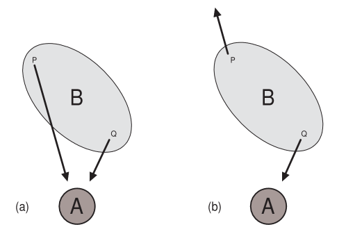
Figure 2: An extended object, B, acted on by the gravitational field of a nearby object, A. (a) depicts the forces as seen from the point of view of the forcing object: both points P and Q fall towards the A, albeit at different rates. (b) depicts the forces as seen from the point of view of the mass center of B where both P and Q recede from the mass center.

In order to appreciate these problems it is helpful to look at a simplified version of the tidal model as proposed by Peebles. Consider two neighbouring, similar sized, protogalaxies A and B (figure  2). We can view the tidal forces exerted on B by A from either the reference frame of the mass center of A or from the reference frame of the mass center of B itself. These forces are depicted by arrows in the figure: note that relative to the mass center of B the tidal forces act so as to stretch B out in the direction of A.

To a first approximation, the force gradient acting on B can be expressed in terms of the potential field $\phi(\bf x)$ in which B is situated:

$$T_{ij}=\displaystyle{\partial{F_{i}}\over\partial{x_{j}}}=\displaystyle{{{\partial^{2}\phi}\over{\partial x_{i}\partial x_{j}}}}-{1\over 3}\delta_{ij}\nabla^{2}\phi$$ (1)

where the potential field is determined from the fluctuating component of the density field via the Poisson equation . The flow of material is thus a shear flow determined by the principal directions and magnitudes of inertia tensor of the blob B. Viewed as a fluid flow this is undeniably a shear flow with zero vorticity as demanded by the Kelvin circulation theorem .

So how does the vorticity that is evident in galaxy rotation arise? The answer is twofold. Shocks will develop in the gas flow and stars will form: the Kelvin Theorem holds only for nondissipative flows. Then, a “gas” of stars does not obey the Kelvin Theorem since it is not a fluid (though there is a six-dimensional phase space analogue for a stellar “gas”).

The magnitude and direction of angular momentum vector is related to the inertia tensor. $I_{ij}$, of the torqued object and the driving tidal forces described by the tensor $T_{ij}$ of equation (1). In 1984, based on simple low-order perturbation theory, White (1984) wrote an intuitively appealing expression for the angular momentum vector $L_{i}$ of a protogalaxy having inertia tensor $I_{mk}$:

$$L_{i}\propto\epsilon_{ijk}T_{jm}I_{mk},$$ (2)

where summation is implied over the repeated indices. This was later taken up by Catelan & Theuns (1999) in a high-order perturbation theory discussion of the problem. However, there is in these treatments an underlying assumption, discussed but dismissed by Catelan & Theuns (1999), that the tensors $T_{ij}$ and $I_{ij}$ are statistically independent. Subsequent numerical work by Lee & Pen (2000) showed that this assumption is not correct and that ignoring it results in an incorrect estimator for the magnitude of the spin.

The approach taken by Lee & Pen (2000, 2001) is interesting: they write down an equation for the autocorrelation tensor of the angular momentum vector in a given tidal field, averaging over all orientations and magnitudes of the inertia tensor. On the basis of equation (2) one would expect this tensor autocorrelation function to be given by

$$\langle L_{i}L_{j}|{\bf T}\rangle\propto\epsilon_{ipq}\epsilon_{jrs}T_{pm}T_{rn}\langle I_{mq}I_{ns}\rangle$$ (3)

where the notation $\langle L_{i}L_{j}|{\bf T}\rangle$ is used to emphasise that $T_{ij}$ is regarded as a given value and is not a random variable. The argument then goes that the isotropy of underlying density distribution allows us to replace the statistical quantity $\langle I_{mq}I_{ns}\rangle$ by a sum of Kronecker deltas leaving only

$$\langle L_{i}L_{j}|{\bf T}\rangle\propto{1\over 3}\delta_{ij}+({1\over 3}\delta_{ij}-T_{ik}T_{kj})$$ (4)

It is then asserted that if the moment of inertia and tidal shear tensors were uncorrelated, we would have only the first term on the right hand side, ${1\over 3}\delta_{ij}$: the angular momentum vector would be isotropically distributed relative to the tidal tensor.

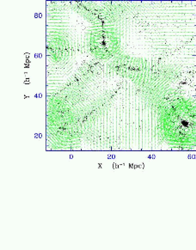
Figure 4: The relation between the cosmic web, the clusters at the nodes in this network and the corresponding compressional tidal field pattern. It shows the matter distribution at the present cosmic epoch, along with the (compressional component) tidal field bars in a slice through a simulation box containing a realization of cosmic structure formed in an open, $\Omega_{\circ}=0.3$, Universe for a CDM structure formation scenario (scale: $R_{G}=2h^{-1}\hbox{\rm Mpc}$). The frame shows structure in a $5h^{-1}\hbox{\rm Mpc}$ thin central slice, on which the related tidal bar configuration is superimposed. The matter distribution, displaying a pronounced weblike geometry, is clearly intimately linked with a characteristic coherent compressional tidal bar pattern. From: van de Weygaert 2002

In fact, in the primordial density field and the early linear phase of structure formation there is a significant correlation between the shape of density fluctuations and the tidal force field (Bond, 1987; van de Weygaert & Bertschinger, 1996). Part of the correlation is due to the anisotropic shape of density peaks and the internal tidal gravitational force field that goes along with it (Icke, 1973). The most significant factor is that of intrinsic spatial correlations in the primordial density field. It is these intrinsic correlations between shape and tidal field that are at the heart of our understanding of the Cosmic Web, as has been recognized by the Cosmic Web theory of Bond et al. (1996). The subsequent nonlinear evolution may strongly augment these correlations (see e.g. fig. 4), although small-scale highly nonlinear interactions also lead to a substantial loss of the alignments: clusters are still strongly aligned, while galaxies seem less so.

Recognizing that the inertia and tidal tensors may not be mutually independent, Lee & Pen (2000, 2001) write

$$\langle L_{i}L_{j}|{\bf T}\rangle\propto{1\over 3}\delta_{ij}+c({1\over 3}\delta_{ij}-T_{ik}T_{kj})$$ (5)

where $c=0$ for randomly distributed angular momentum vectors. The case of mutually independent tidal and inertia tensors is described by $c=1$ (see equation 4). They finally introduce a different parameter $a=3c/5$ and write

$$\langle L_{i}L_{j}|{\bf T}\rangle\propto{{1+a}\over 3}\delta_{ij}-aT_{ik}T_{kj}$$ (6)

which forms the basis of much current research in this field. The value derived from recent study of the Millenium simulations by Lee & Pen (2007) is $a\approx 0.1$.

3 Gravitational Instability

In the gravitational instability scenario, (e.g. Peebles, 1980), cosmic structure grows from an intial random field of primordial density and velocity perturbations. The formation and molding of structure is fully described by three equations, the continuity equation, expressing mass conservation, the Euler equation for accelerations driven by the gravitational force for dark matter and gas, and pressure forces for the gas, and the Poisson-Newton equation relating the gravitational potential to the density.

A general density fluctuation field for a component of the universe with respect to its cosmic background mass density $\rho_{\rm u}$ is defined by

$$\delta({\bf r},t)\,=\,\frac{\rho({\bf r})-\rho_{\rm u}}{\rho_{\rm u}}\,.$$ (7)

Here ${\bf r}$ is comoving position, with the average expansion factor $a(t)$ of the universe taken out. Although there are fluctuations in photons, neutrinos, dark energy, etc., we focus here on only those contributions to the mass which can cluster once the relativistic particle contribution has become small, valid for redshifts below 100 or so. A non-zero $\delta({\bf r},t)$ generates a corresponding total peculiar gravitational acceleration ${\bf g}({\bf r})$ which at any cosmic position ${\bf r}$ can be written as the integrated effect of the peculiar gravitational attraction exerted by all matter fluctuations throughout the Universe:

$${\bf g}({\bf r},t)\,=\,-4\pi G\bar{\rho}_{m}(t)a(t)\int{\rm d}{\bf r}^{\prime}\,\delta({\bf r}^{\prime},t)\,{\displaystyle({\bf r}-{\bf r}^{\prime})\over\displaystyle|{\bf r}-{\bf r}^{\prime}|^{3}}\ .$$ (8)

Here $\bar{\rho}_{m}(t)$ is the mean density of the mass in the universe that can cluster (dark matter and baryons). The cosmological density parameter $\Omega_{m}(t)$ is defined by $\rho_{\rm u}$, via the relation $\Omega_{m}H^{2}=(8\pi G/3)\bar{\rho_{m}}$ in terms of the Hubble parameter $H$. The relation between the density field and gravitational potential $\Phi$ is established through the Poisson-Newton equation:

$$\nabla^{2}\Phi=4\pi G\bar{\rho}_{m}(t)a(t)^{2}\ \delta({\bf r},t).$$ (9)

The peculiar gravitational acceleration is related to $\Phi({\bf r},t)$ through ${\bf g}=-\nabla\Phi/a$ and drives peculiar motions.

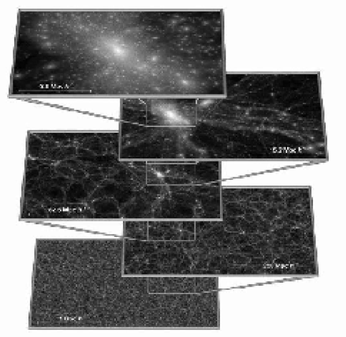
Figure 3: The hierarchical Cosmic Web: over a wide range of spatial and mass scales structures and features are embedded within structures of a larger effective dimension and a lower density. Image courtesy of V. Springel & Virgo consortium, also see Springel et al. 2005. Reproduced with permission of Nature.

In slightly overdense regions around density excesses, the excess gravitational attraction slows down the expansion relative to the mean, while underdense regions expand more rapidly. The underdense regions around density minima expand relative to the background, forming deep voids. Once the gravitational clustering process has progressed beyond the initial linear growth phase we see the emergence of complex patterns and structures in the density field.

Large N-body simulations all reveal a few “universal” characteristics of the (mildly) nonlinear cosmic matter distribution: its hierarchical nature, the anisotropic and weblike spatial geometry of the spatial mass distribution and the presence of huge underdense voids. These basic elements of the Cosmic Web (Bond et al., 1996; van de Weygaert & Bond, 2008) exist at all redshifts, but differ in scale.

Fig. 3, from the state-of-the-art “Millennium simulation”, illustrates this complexity in great detail over a substantial range of scales. The figure zooms in on the dark matter distribution at five levels of spatial resolution and shows the formation of a filamentary network connecting to a central cluster. This network establishes transport channels along which matter will flow into the cluster. The hierarchical nature of the structure is clearly visible. The dark matter distribution is far from homogeneous: a myriad of tiny dense clumps indicate the presence of dark halos in which galaxies, or groups of galaxies, will have formed.

Within the context of gravitational instability, it is the gravitational tidal forces that establish the relationship between some of the most prominent manifestations of the structure formation process. It is this intimate link between the Cosmic Web, the mutual alignment between cosmic structures and the rotation of galaxies to which we wish to draw attention in this short contribution.

4 Tidal Shear

When describing the dynamical evolution of a region in the density field it is useful to distinguish between large scale “background” fluctuations $\delta_{\rm b}$ and small-scale fluctuations $\delta_{\rm f}$. Here, we are primarily interested in the influence of the smooth large-scale field. Its scale $R_{b}$ should be chosen such that it remains (largely) linear, i.e. the r.m.s. density fluctuation amplitude $\sigma_{\rho}(R_{b},t)\lesssim 1$.

To a good approximation the smoother background gravitational force ${\bf g}_{\rm b}({\bf x})$ (eq. 8) in and around the mass element includes three components (apart from rotational aspects). The bulk force ${\bf g}_{\rm b}({\bf x}_{pk})$ is responsible for the acceleration of the mass element as a whole. Its divergence ($\nabla\cdot{\bf g}_{\rm b}$) encapsulates the collapse of the overdensity while the tidal tensor $T_{ij}$ quantifies its deformation,

$$g_{\rm b,i}({\bf x})\,=\,g_{\rm b,i}({\bf x}_{pk})\,+\,a\,\sum_{j=1}^{3}\,\left\{{\displaystyle 1\over\displaystyle 3a}(\nabla\cdot{\bf g}_{\rm b})({\bf x}_{pk})\,\delta_{\rm ij}\,-\,T_{ij}\right\}(x_{j}-x_{pk,{\rm j}})\,.$$ (10)

The tidal shear force acting over the mass element is represented by the (traceless) tidal tensor $T_{ij}$,

$$T_{\rm ij} \,\equiv\, -{\displaystyle 1\over\displaystyle 2a}\,\left\{{\displaystyle\partial g_{{\rm b},i}\over\displaystyle\partial x_{i}}+{\displaystyle\partial g_{{\rm b},j}\over\displaystyle\partial x_{j}}\right\}\,+\,{\displaystyle 1\over\displaystyle 3a}(\nabla\cdot{\bf g}_{\rm b})\,\delta_{\rm ij}$$ (11)

in which the trace of the collapsing mass element, proportional to its overdensity $\delta$, dictates its contraction (or expansion). For a cosmological matter distribution the close connection between local force field and global matter distribution follows from the expression of the tidal tensor in terms of the generating cosmic matter density fluctuation distribution $\delta({\bf r})$ (van de Weygaert & Bertschinger, 1996):

$$T_{ij}({\bf r})={\displaystyle 3\Omega H^{2}\over\displaystyle 8\pi}\,\int{\rm d}{\bf r}^{\prime}\,\delta({\bf r}^{\prime})\ \left\{{\displaystyle 3(r_{i}^{\prime}-r_{i})(r_{j}^{\prime}-r_{j})-|{\bf r}^{\prime}-{\bf r}|^{2}\ \delta_{ij}\over\displaystyle|{\bf r}^{\prime}-{\bf r}|^{5}}\right\}-{\frac{1}{2}}\Omega H^{2}\ \delta({\bf r},t)\ \delta_{ij}.$$

The tidal shear tensor has been the source of intense study by the gravitational lensing community since it is now possible to map the distribution of large scale cosmic shear using weak lensing data. See for example Hirata & Seljak (2004); Massey et al. (2007).

5 The Cosmic Web

Perhaps the most prominent manifestation of the tidal shear forces is that of the distinct weblike geometry of the cosmic matter distribution, marked by highly elongated filamentary, flattened planar structures and dense compact clusters surrounding large near-empty void regions (see fig. 3). The recognition of the Cosmic Web as a key aspect in the emergence of structure in the Universe came with early analytical studies and approximations concerning the emergence of structure out of a nearly featureless primordial Universe. In this respect the Zel’dovich formalism (Zeldovich, 1970) played a seminal role. It led to the view of structure formation in which planar pancakes form first, draining into filaments which in turn drain into clusters, with the entirety forming a cellular network of sheets.

The Megaparsec scale tidal shear forces are the main agent for the contraction of matter into the sheets and filaments which trace out the cosmic web. The anisotropic contraction of patches of matter depends sensitively on the signature of the tidal shear tensor eigenvalues. With two positive eigenvalues and one negative, $(-++)$, we will see strong collapse along two directions. Dependent on the overall overdensity, along the third axis collapse will be slow or not take place at all. Likewise, a sheetlike membrane will be the product of a $(--+)$ signature, while a $(+++)$ signature inescapably leads to the full collapse of a density peak into a dense cluster.

For a proper understanding of the Cosmic Web we need to invoke two important observations stemming from intrinsic correlations in the primordial stochastic cosmic density field. When restricting ourselves to overdense regions in a Gaussian density field we find that mildly overdense regions do mostly correspond to filamentary $(-++)$ tidal signatures (Pogosyan et al., 1998). This explains the prominence of filamentary structures in the cosmic Megaparsec matter distribution, as opposed to a more sheetlike appearance predicted by the Zeld’ovich theory. The same considerations lead to the finding that the highest density regions are mainly confined to density peaks and their immediate surroundings.

The second, most crucial, observation (Bond et al., 1996) is the intrinsic link between filaments and cluster peaks. Compact highly dense massive cluster peaks are the main source of the Megaparsec tidal force field: filaments should be seen as tidal bridges between cluster peaks. This may be directly understood by realizing that a $(-++)$ tidal shear configuration implies a quadrupolar density distribution (eqn. 4). This means that an evolving filament tends to be accompanied by two massive cluster patches at its tip. These overdense protoclusters are the source of the specified shear, explaining the canonical cluster-filament-cluster configuration so prominently recognizable in the observed Cosmic Web.

6 the Cosmic Web and Galaxy Rotation: MMF analysis

With the cosmic web as a direct manifestation of the large scale tidal field we may wonder whether we can detect a connection with the angular momentum of galaxies or galaxy halos. In section 2 we have discussed how tidal torques generate the rotation of galaxies. Given the common tidal origin we would expect a significant correlation between the angular momentum of halos and the filaments or sheets in which they are embedded. It was Lee & Pen (2000) who pointed out that this link should be visible in alignment of the spin axis of the halos with the inducing tidal tensor, and by implication the large scale environment in which they lie.

In order to investigate this relationship it is necessary to isolate filamentary features in the cosmic matter distribution. A systematic morphological analysis of the cosmic web has proven to be a far from trivial problem, though there have recently been some significant advances. Perhaps the most rigorous program, with a particular emphasis on the description and analysis of filaments, is that of the skeleton analysis of density fields by Novikov, Colombi & Doré (2006); Sousbie et al. (2007). Another strategy has been followed by Hahn et al. (2007) who identify clusters, filaments, walls and voids in the matter distribution on the basis of the tidal field tensor $\partial^{2}\phi/\partial x_{i}\partial x_{j}$, determined from the density distribution filtered on a scale of $\approx 5h^{-1}\hbox{\rm Mpc}$.

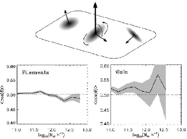
Figure 5: Average alignment angle $\cos\theta$ between the halo spin direction and the orientation of the host structure as a function of halo mass, for filaments (left) and walls (right) in a $\Lambda$CDM N-body simulation. Filaments and walls were identified using the MMF technique. The dotted line indicates a uniform distribution of halo orientations. The shaded area corresponds to the standard deviation of 1000 random realisations with the same number of galaxies as the halo sample and is wider in the case of walls due to the lower number of haloes in walls. From Aragón-Calvo et al. (2007).

The one method that explicitly takes into account the hierarchical nature of the mass distribution when analyzing the weblike geometries is the Multiscale Morphology Filter (MMF), introduced by Aragón-Calvo et al. (2007). The MMF dissects the cosmic web on the basis of the multiscale analysis of the Hessian of the density field. It starts by translating an N-body particle distribution or a spatial galaxy distribution into a DTFE density field (see van de Weygaert & Schaap, 2007). This guarantees a morphologically unbiased and optimized density field retaining all features visible in a discrete galaxy or particle distribution. The DTFE field is filtered over a range of scales. By means of morphology filter operations defined on the basis of the Hessian of the filtered density fields the MMF successively selects the regions which have a bloblike (cluster) morphology, a filamentary morphology and a planar morphology, at the scale at which the morphological signal is optimal. By means of a percolation criterion the physically significant filaments are selected. Following a sequence of blob, filament and wall filtering finally produces a map of the different morphological features in the particle distribution.

With the help of the MMF we have managed to find the relationship of shape (inertia tensor) and spin-axis of halos in filaments and walls and their environment. On average, the long axis of filament halos is directed along the axis of the filament; wall halos tend to have their longest axis in the plane of the wall. At the present cosmic epoch the effect is stronger for massive halos. Interestingly, the trend appears to change in time: low mass halos tended to be more strongly aligned but as time proceeds local nonlinear interactions affect the low mass halos to such an extent that the situation has reversed.

The orientation of the rotation axis provides a more puzzling picture (fig. 5). The rotation axis of low mass halos tends to be directed along the filament’s axis while that of massive halos appears to align in the perpendicular direction. In walls there does not seem to exist such a bias: the rotation-axis of both massive and light haloes tends to lie in the plane of the wall. At earlier cosmic epochs the trend in filaments was entirely different: low mass halo spins were more strongly aligned as large scale tidal fields were more effective in directing them. During the subsequent evolution in high-density areas, marked by strongly local nonlinear interactions with neighbouring galaxies, the alignment of the low mass objects weakens and ultimately disappears.

7 Tidal Fields and Void alignment

A major manifestation of large scale tidal influences is that of the alignment of shape and angular momentum of objects (see Bond et al., 1996; Desjacques, 2007). The alignment of the orientations of galaxy haloes, galaxy spins and clusters with larger scale structures such as clusters, filaments and superclusters has been the subject of numerous studies (see e.g. Binggeli, 1982; Bond, 1987; Rhee et al., 1991; Plionis & Basilakos, 2002; Basilakos et al., 2006; Trujillo et al., 2006; Aragón-Calvo et al., 2007; Lee & Evrard, 2007; Lee et al., 2007).

Voids are a dominant component of the Cosmic Web (see e.g. Tully et al., 2007; Romano-Díaz & van de Weygaert, 2007), occupying most of the volume of space. Recent analytical and numerical work (Park & Lee, 2007; Lee & Park, 2007; Platen, van de Weygaert & Jones, 2008) discussed the magnitude of the tidal contribution to the shape and alignment of voids. Lee & Park (2007) found that the ellipticity distribution of voids is a sensitive function of various cosmological parameters and remarked that the shape evolution of voids provides a remarkably robust constraint on the dark energy equation of state. Platen, van de Weygaert & Jones (2008) presented evidence for significant alignments between neigbouring voids, and established the intimate dynamic link between voids and the cosmic tidal force field.

Voids were identified with the help of the Watershed Void Finder (WVF) procedure (Platen, van de Weygaert & Jones, 2007). The WVF technique is based on the topological characteristics of the spatial density field and thereby provides objectively defined measures for the size, shape and orientation of void patches.

7.1 Void-Tidal Field alignments: formalism

In order to trace the contributions of the various scales to the void correlations Platen, van de Weygaert & Jones (2008) investigated the alignment between the void shape and the tidal field smoothed over a range of scales $R$. The alignment function ${\mathcal{A}}_{TS}(R_{1})$ between the local tidal field tensor $T_{ij}(R_{1})$, Gaussian filtered on a scale $R_{1}$ at the void centers, and the void shape ellipsoid is determined as follows.

Figure 6: Left: on the landscape with WVF void boundaries the tidal field compressional component is represented by tidal bars (red), representing the direction and strength of the tidal field. Also depicted are the void shape bars (blue). Right: the dotted line shows $\mathcal{C}_{TS}$, the alignment between the compressional direction of the tidal field and the shortest shape axis. For comparison the short axis alignment is also superimposed. From Platen et al. 2008.

For each individual void region the shape-tensor $\mathcal{S}_{ij}$ is calculated by summing over the $N$ volume elements $k$ located within the void,

$$\qquad\mathcal{S}_{ij} =- \sum_{k}x_{ki}x_{kj}\qquad\ \ \ \ \ \ \ \ \textrm{(offdiagonal)}$$ (12)

$$\qquad\mathcal{S}_{ii} = \sum_{k}\left({\bf x}_{k}^{2}-x_{ki}^{2}\right)\qquad\ \ \textrm{(diagonal)}\,,$$

where ${\bf x}_{k}$ is the position of the $k$-th volume element within the void, with respect to the (volume-weighted) void center ${\bf{\overline{r}}}_{v}$, i.e. ${\bf x}_{k}={\bf r}_{k}-{\bf{\overline{r}}}_{v}$. The shape tensor $\mathcal{S}_{ij}$ is related to the inertia tensor $\mathcal{I}_{ij}$. However, it differs in assigning equal weight to each volume element within the void region. Instead of biasing the measure towards the mass concentrations near the edge of voids, the shape tensor $\mathcal{S}_{ij}$ yields a truer reflection of the void’s interior shape.

The smoothing of the tidal field is done in Fourier space using a Gaussian window function ${\hat{W}}^{*}({\bf k};R)$:

$$T_{ij}({\bf r};R)\,=\,{\displaystyle 3\over\displaystyle 2}\Omega H^{2}\int{\displaystyle{\rm d}{\bf k}\over\displaystyle(2\pi)^{3}}\left({\displaystyle k_{i}k_{j}\over\displaystyle k^{2}}-{\displaystyle 1\over\displaystyle 3}\delta_{ij}\right)\,{\hat{W}}^{*}({\bf k};R)\,{\hat{\delta}}({\bf k})\,{\rm e}^{-{\rm i}{\bf k}\cdot{\bf r}}$$

Here, ${\hat{\delta}}({\bf k})$ is the Fourier amplitude of the relative density fluctuation field at wavenember $\bf k$.

Given the void shape ${\mathcal{S}}_{ij}$ and the tidal tensor $T_{ij}$, for every void the function ${\Gamma}_{TS}(m,R_{1})$ at the void centers is determined:

$${\Gamma}_{TS}(m;R_{1}) \,=\, \ -\ {\displaystyle\sum\nolimits_{i,j}{\tilde{\mathcal{S}}}_{m,ij}\,T_{ij}({\bf r}_{m};R_{1})\over\displaystyle{\tilde{\mathcal{S}}}_{m}\,\,T({\bf r}_{m};R_{1})}$$ (13)

where $T({\bf r}_{m};R_{1})$ is the norm of the tidal tensor $T_{ij}({\bf r_{m}})$ filtered on a scale $R_{1}$ and

The void-tidal alignment ${\mathcal{A}}_{TS}(R_{1})$ at a scale $R$ is then the ensemble average

$${\mathcal{A}}_{TS}(R_{1}) \,=\, \langle\,\Gamma_{TS}(R_{1})\,\rangle\,.$$ (14)

which we determine simply by averaging $\Gamma_{TS}(m,R_{1})$ over the complete sample of voids.

7.2 Void-Tidal Field alignments: results

A visual impression of the strong relation between the void’s shape and orientation and the tidal field is presented in the lefthand panel of fig 6 (from Platen, van de Weygaert & Jones (2008)). The tidal field configuration is depicted by means of (red-coloured) tidal bars. These bars represent the compressional component of the tidal force field in the slice plane, and have a size proportional to its strength and are directed along the corresponding tidal axis. The bars are superimposed on the pattern of black solid watershed void boundaries, whose orientation is emphasized by means of a bar directed along the projection of their main axis.

The compressional tidal forces tend to be directed perpendicular to the main axis of the void. This is most clearly in regions where the forces are strongest and most coherent. In the vicinity of great clusters the voids point towards these mass concentrations, stretched by the cluster tides. The voids that line up along filamentary structures, marked by coherent tidal forces along their ridge, are mostly oriented along the filament axis and perpendicular to the local tidal compression in these region. The alignment of small voids along the diagonal running from the upper left to the bottom right is particularly striking.

A direct quantitative impression of the alignment between the void shape and tidal field, may be obtained from the righthand panel of fig. 6. The figure shows $\mathcal{C}_{TS}$ (dotted line), the alignment between the compressional direction of the tidal field and the shortest shape axis. It indicates that the tidal field is instrumental in aligning the voids. To further quantify and trace the tidal origin of the alignment one can investigate the local shape-tide alignment function ${\mathcal{A}}_{TS}$ (eqn. 14) versus the smoothing radius $R_{1}$.

This analysis reveals that the alignment remains strong over the whole range of smoothing radii out to $R_{1}\approx 20-30h^{-1}\hbox{\rm Mpc}$ and peaks at a scale of $R_{1}\approx 6h^{-1}\hbox{\rm Mpc}$. This scale is very close to the average void size, and also close to the scale of nonlinearity. This is not a coincidence: the identifiable voids probe the linear-nonlinear transition scale. The remarkably strong alignment signal at large radii than $R_{1}>20h^{-1}\hbox{\rm Mpc}$ (where ${\mathcal{A}}_{TS}\approx 0.3$), can only be understood if large scale tidal forces play a substantial role in aligning the voids.

8 Final remarks

The last word on the origin of galactic angular momentum has not been said yet. It is now a part of our cosmological paradigm that the global tidal fields from the irregular matter distribution on all scales is the driving force, but the details of how this works have yet to be explored. That is neither particularly demanding nor particularly difficult, it is simply not trendy: there are other problems of more pressing interest. The transition from shear dominated to rotation dominated motion is hardly explored and will undoubtedly be one of the principal by-products of cosmological simulations with gas dynamics and star formation.

The role of tidal fields has been found to be more profound than the mere transfer of angular momentum to proto-objects. The cosmic tidal fields evidently shape the entire distribution and dynamics of galaxies: they shape what has become known as the “cosmic web”. Although we see angular momentum generation in cosmological N-Body simulations it is not clear that the simulations do much more than tell us what happened: galaxy haloes in N-Body models have acquired spin by virtue of tidal interaction. We draw comfort from the fact that the models give the desired result.

Nikos Voglis’ approach was somewhat deeper: he wanted to understand things at a mechanistic level rather than simply to simulate them and observe the result. In that he stands in the finest tradition of the last of the great Hellenistic scientists, Hipparchus of Nicaea, who studied motion of bodies under gravity. Perhaps we should continue in the spirit of Nikos’ work by trying to understand things rather than simply simulate them.

Nikos was a good friend, a fine scientist and certainly one of the kindest people one could ever meet. It was less than one year ago when we met for the last time at the bernard60 conference in Valencia. We were of course delighted to see him and we shall cherish that brief time together.

9 Acknowledgments

We thank Panos Patsis and George Contopoulos for the opportunity of delivering this tribute to our late friend. We are grateful to Volker Springel for allowing us to use figure 3. We particularly wish to acknowledge Miguel Aragón-Calvo and Erwin Platen for allowing us to use their scientific results: their contributions and discussions have been essential for our understanding of the subject.

References

- Aragón-Calvo et al. (2007) Aragón-Calvo M.A., Jones B.J.T., van de Weygaert R., van der Hulst J.M.: Astrophys. J. 655, L5 (2007)
- Aragón-Calvo et al. (2007) Aragón-Calvo M.A., Jones B.J.T., van de Weygaert R., van der Hulst J.M.: Astron. Astrophys. 474, 315 (2007)
- Barnes & Efstathiou (1987) Barnes J., Efstathiou G.: Astrophys. J. 319, 575 (1987)
- Basilakos et al. (2006) Basilakos S., Plionis M., Yepes G., Gottlöber S., Turchaninov V.: Mon. Not. Roy. Astron. Soc. 365, 539 (2006)
- (5) Bett P., Eke V., Frenk C.S., Jenkins A., Helly J., Navarro J.: Mon. Not. Roy. Astron. Soc. 376, 215 (2007)
- Binggeli (1982) Binggeli B.: Astron. Astrophys. 107, 338 (1982)
- Bond (1987) Bond J.R.: in Nearly Normal Galaxies, ed. S. Faber (Springer, New York), p. 388 (1987)
- Bond et al. (1996) Bond J. R., Kofman L., Pogosyan D.: Nature 380, 603 (1996)
- Catelan & Theuns (1999) Catelan, P., and Theuns, T.: Mon. Not. Roy. Astron. Soc. 282, 436 (1999)
- Desjacques (2007) Desjacques V.: arXiv0707.4670 (2007)
- Doroshkevich (1970) Doroshkevich A.G.: Astrophysics 6, 320 (1970)
- Efstathiou & Jones (1979) Efstathiou G., Jones B. J. T.: Mon. Not. Roy. Astron. Soc. 186, 133 (1979)
- Feynman (1970) Feynman, R.P.: Feynman Lectures On Physics, (Addison Wesley Longman) (1970)
- Hahn et al. (2007) Hahn O., Porciani C., Carollo M., Dekel A.: Mon. Not. R. Astron. Soc. 375, 489 (2007)
- (15) Harrison, E.R.: Mon. Not. Roy. Astron. Soc. 154, 167 (1971)
- Hirata & Seljak (2004) Hirata C.M., Seljak U.: Phys. Rev. D, 70, 063526 (2004)
- Hoyle (1949) Hoyle F.: in Problems of Cosmical Aerodynamics, ed. J. M. Burgers and H. C. van de Hulst (Dayton: Central Air Documents Office), 195 (1949)
- Icke (1973) Icke V.: Astron. Astrophys. 27, 1 (1973)
- Jones (1976) Jones B.J.T.: Rev. Mod. Phys. 48, 107 (1976)
- (20) Jones B. J. T., Efstathiou G.: Mon. Not. Roy. Astron. Soc. 189, 27 (1979)
- Lee & Evrard (2007) Lee J., Evrard A.E.: Astrophys. J. 657, 30 (2007)
- Lee & Park (2007) Lee J., Park D.: arXiv0704.0881 (2007)
- Lee & Pen (2000) Lee J., Pen U.: Astrophys. J. 532, L5 (2000)
- Lee & Pen (2001) Lee J., Pen U.: Astrophys. J. 555, 106 (2001)
- Lee & Pen (2007) Lee J., Pen U.: arXiv0707.1690 (2007)
- Lee et al. (2007) Lee J., Springel V., Pen U-L., Lemson G.: arXiv0709.1106 (2007)
- Massey et al. (2007) Massey R., Rhodes J., Ellis R., Scoville N., Leauthaud A., Finoguenov A., Capak P., Bacon D., Aussel H., Kneib J.-P., Koekemoer A., McCracken H., Mobasher B., Pires S., Refregier A., Sasaki S., Starck J.-L., Taniguchi Y., Taylor A., Taylor J.: Nature 445, 286 (2007)
- Novikov, Colombi & Doré (2006) Novikov D., Colombi S., Doré O.: Mon. Not. R. Astron. Soc. 366, 1201 (2006)
- Oort (1970) Oort J.H.: Astron. Astrophys. 7, 381 (1970)
- Palmer & Voglis (1983) Palmer P.L., Voglis N.: Mon. Not. Roy. Astron. Soc. 205, 543 (1983)
- Park & Lee (2007) Park D. and Lee J.: Astrophys. J. 665, 96 (2007)
- Peebles (1969) Peebles P. J. E.: Astrophys. J. 155, 393 (1969)
- Peebles (1980) Peebles P. J. E.: The large-scale structure of the universe, (Princeton University Press) (1980)
- Platen, van de Weygaert & Jones (2007) Platen E., van de Weygaert R., Jones B.J.T.: Mon. Not. Roy. Astron. Soc. 380, 551 (2007)
- Platen, van de Weygaert & Jones (2008) Platen E., van de Weygaert R., Jones B.J.T.: Mon. Not. R. Astron. Soc., in press (2008)
- Plionis & Basilakos (2002) Plionis M., Basilakos S.: Mon. Not. Roy. Astron. Soc. 329, L47 (2002)
- Pogosyan et al. (1998) Pogosyan D.Yu.m Bond J.R., Kofman L., Wadsley J.: Cosmic Web: Origin and Observables. In: Wide Field Surveys in Cosmology, 14th IAP meeting), eds. S. Colombi, Y. Mellier, (Editions Frontieres, p. 61 (1998)
- Porciani et al. (2002) Porciani C., Dekel A., Hoffman Y.: Mon. Not. Roy. Astron. Soc. 332, 325 (2002)
- Rhee et al. (1991) Rhee G., van Haarlem M., Katgert P.: Astron. J. 103, 6 (1991)
- Romano-Díaz & van de Weygaert (2007) Romano-Díaz E., van de Weygaert R.: Mon. Not. Roy. Astron. Soc. 382, 2 (2007)
- Sousbie et al. (2007) Sousbie T., Pichon C., Colombi S., Novikov D., Pogosyan D.: astroph/07073123 (2007)
- Springel et al. (2005) Springel V., White S.D.M., Jenkins A., Frenk C.S., Yoshida N., Gao L., Navarro J., Thacker R., Croton D., Helly J., Peacock J.A., Cole S., Thomas P., Couchman H., Evrard A., Colberg J.M., Pearce F.: Nature 435, 629 (2005)
- Trujillo et al. (2006) Trujillo I., Carretero C., Patiri S. G.: Astrophys. J. 640, L111 (2006)
- Tully et al. (2007) Tully R.B., Shaya E.J., Karachentsev I.D., Courtois H., Kocevski D.D., Rizzi L., Peel A.: arXiv:0705.4139 (2007)
- van den Bosch et al. (2002) van den Bosch F. C., Abel T., Croft R. A. C., Hernquist L., White S. D. M.: Astrophys. J. 576, 21 (2002)
- van de Weygaert & Bertschinger (1996) van de Weygaert R., Bertschinger E.: Mon. Not. R. Astron. Soc. 281, 84 (1996)
- van de Weygaert & Schaap (2007) van de Weygaert R., Schaap W.E: The Cosmic Web: Geometric Analysis. In: Data Analysis in Cosmology, lectures summerschool Valencia 2004, ed. by V. Martínez, E. Saar, E. Martínez-González, M. Pons-Borderia (Springer-Verlag), 129pp. (2008)
- van de Weygaert & Bond (2008) van de Weygaert R., Bond J.R.: Clusters and the Theory of the Cosmic Web. In: A Pan-Chromatic View of Clusters of Galaxies and the LSS, eds. M. Plionis, D. Hughes, O. López-Cruz (Springer 2008)
- White (1984) White S. D. M.: Astrophys. J. 286, 38 (1984)
- Zeldovich (1970) Zel’dovich Ya. B.: Astron. Astrophys. 5, 84 (1970)