A Universal Map for Fractal Structures in Weak Solitary Wave Interactions

Abstract

Fractal scatterings in weak solitary wave interactions is analyzed for generalized nonlinear Schrödiger equations (GNLS). Using asymptotic methods, these weak interactions are reduced to a universal second-order map. This map gives the same fractal scattering patterns as those in the GNLS equations both qualitatively and quantitatively. Scaling laws of these fractals are also derived.

Solitary wave interactions is a fascinating mathematical phenomenon, and it arises in numerous physical applications such as water waves and nonlinear optics Ablowitz ; Hasegawa ; Kivshar . Strong interactions occur when two solitary waves are initially far apart but move toward each other at moderate or large speeds. Weak interactions would occur if the two waves are initially well separated, and their relative velocities are small. In integrable wave equations, strong interactions of solitary waves are elastic, and their weak interactions exhibit interesting but simple dynamics Ablowitz ; Hasegawa ; Karpman_Solovev . In non-integrable systems, however, solitary wave interactions can be extremely complicated. Indeed, one of the most important developments in the nonlinear wave theory in recent years is the discovery of fractal scatterings of solitary wave interactions in non-integrable equations Campbell ; anninos ; Kivshar_Fei ; YangTan ; Dmitriev ; zhuyang ; Goodman_Haberman . On the analysis of fractal scatterings, some progress has been made. For strong interactions, various collective-coordinate ODE models based on qualitative variational methods have been derived and analyzed anninos ; Kivshar_Fei ; YangTan ; Goodman_Haberman . From the variational ODEs, a separatrix map was derived, showing chaotic scatterings [11]. On weak interactions, a simple asymptotically-accurate ODE model was derived for the generalized NLS equations zhuyang . This ODE system offered the first glimpse of universal fractal scatterings in weak wave interactions, but these fractal patterns were not analyzed.

In this letter, we analyze fractal scattering patterns in weak solitary wave interactions for generalized nonlinear Schrödiger equations. Using asymptotic methods, we reduce these weak interactions to a simple second-order map which contains no free parameters. It is shown that this universal map gives a complete characterization of fractal structures in these wave interactions. In addition, the scaling laws of these fractals for different initial conditions are analytically derived. These results provide a deep understanding of weak solitary-wave interactions for various physical applications.

The generalized nonlinear Schrödinger equations we consider in this paper are

$$iU_{t}+U_{xx}+F(|U|^{2})U=0,$$ (1)

where $F(\cdot)$ is a general function. These equations govern various physical wave phenomena in nonlinear optics, fiber communications and fluid dynamics Ablowitz ; Hasegawa ; Kivshar . This equation admits solitary waves of the form $U=\Phi(x-\xi)e^{i\phi}$, where $\Phi(\theta)$ is a localized positive function, $\xi=Vt+x_{0}$ is the wave’s center position, and $\phi=\frac{1}{2}V(x-\xi)+(\beta+\frac{1}{4}V^{2})t-\eta_{0}$ is the wave’s phase. This wave has four free parameters: velocity $V$, amplitude parameter $\beta$, initial position $x_{0}$, and initial phase $\eta_{0}$. In weak interactions, two such solitary waves are initially well separated and have small relative velocities and amplitude differences. Then they would interfere with each other through tail overlapping. When time goes to infinity, they either separate from each other or form a bound state. The exit velocity, defined as $\Delta V_{\infty}=|V_{2}-V_{1}|_{t\to\infty}$, depends on the initial conditions of the two waves.

To study weak interactions in Eq. (1), we select two different nonlinearities which are cubic-quintic and quadratic-cubic respectively:

$$F(|U|^{2})=|U|^{2}+\gamma|U|^{4},\quad F(|U|^{2})=|U|^{2}+\delta|U|.$$ (2)

Here $\gamma$ and $\delta$ are real parameters. To illustrate results of weak interactions, we take $\gamma=0.0003$ and $\delta=-0.0015$. The initial conditions are taken as

$$x_{0,1}=-x_{0,2}=-5,\;V_{0,k}=0,\;\beta_{0,k}=1\>(k=1,2),$$ (3)

$\phi_{0,1}=0$, and the initial phase difference $\Delta\phi_{0}=\phi_{0,2}-\phi_{0,1}$ is used as the control parameter. In our numerical simulations of Eq. (1), the discrete Fourier transform is used to evaluate the spatial derivative $\partial_{xx}$, while the fourth-order Runge-Kutta method is used to advance in time. The exit velocity $\Delta V_{\infty}$ versus $\Delta\phi_{0}$ graphs for these two nonlinearities are plotted in Fig. 1. These graphs are fractals zhuyang . It is amazing that these fractals appear for such small values of $\gamma$ and $\delta$, where Eq. (1) is simply a weakly perturbed NLS equation. Notice that the fractals for these two different nonlinearities are very similar, signaling their universality in weak wave interactions.

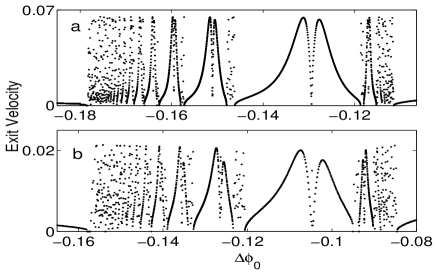
Figure 1: Exit velocity versus initial phase difference graphs for initial conditions (3): (a) cubic-quintic nonlinearity; (b) quadratic-cubic nonlinearity.

To analyze this fractal-scattering phenomena, the Karpman-Solov’ev method Karpman_Solovev was applied, and the following simple set of dynamical equations for solitary wave parameters were derived zhuyang :

$$\zeta_{\tau\tau}=\cos{\psi}e^{\zeta},\quad\psi_{\tau\tau}=(1+\varepsilon)\sin{\psi}e^{\zeta}.$$ (4)

Here $\psi=\Delta\phi$, $\zeta=-\sqrt{\beta}\Delta\xi$,

$$\tau=\sqrt{16\beta^{3/2}c^{2}/P}\;t,\;\;\varepsilon=P/(2\beta P_{\beta})-1,$$ (5)

$\Delta\xi$ and $\Delta\phi$ are the distance and phase difference between the two waves, $\beta=(\beta_{1,0}+\beta_{2,0})/2$, $c$ is the tail coefficient of the solitary wave with propagation constant $\beta$, and $P(\beta)$ is the power function of the wave. These reduced ODEs capture fractal scatterings of weak wave interactions such as in Fig. 1 both qualitatively and quantitatively zhuyang , and they represent an important first step toward the understanding of these phenomena. However, the fractal structures in the PDEs (1) and ODEs (4) have not been analyzed previously. Below we give a complete characterization for the first time of this fractal scattering by analyzing the ODEs (4).

If $\varepsilon=0$, Eq. (4) is integrable. It has two conserved quantities, energy $E$ and momentum $M$:

$$E=(\dot{\zeta}^{2}-\dot{\psi}^{2})/2-e^{\zeta}\cos{\psi},\quad M=\dot{\zeta}\dot{\psi}-e^{\zeta}\sin{\psi}.$$ (6)

Introducing two complex quantities

$$C=\sqrt{(E+iM)/2},\;F=-\mbox{acoth}[(\dot{\zeta}+i\dot{\psi})/2C)]/C,$$ (7)

the analytical solution of Eq. (4) can be found to be

$$Y(\tau)=\ln\left[2C^{2}_{0}\textrm{csch}^{2}C_{0}(\tau-\tau_{0}+F_{0})\right],$$ (8)

where $Y=\zeta+i\psi$, and $C_{0}$, $F_{0}$ are the initial values of $C$ and $F$. The third conserved quantity of Eq. (4) is $\mbox{Im}(F)$. Behaviors of the above integrable solutions should be noted. When $E>0$, or $E\leq 0$ but $M\neq 0$, $\zeta\to-\infty$ (a degenerate saddle point) as $\tau\to\infty$, and thus these solutions are escape orbits. When $E<0$ and $M=0$, the orbits are periodic with period $T_{p}=\sqrt{2}\pi/\sqrt{|E|}$. Orbits with $E=M=0$ separate the escape orbits from the periodic ones, hence we call them separatrix orbits. The formulae for separatrix orbits can be readily found to be

$$Y_{s}(\tau)=-\ln[\sigma A^{-1/2}i+(\tau-\tau_{M})/\sqrt{2}]^{2}.$$ (9)

Here $A=e^{\zeta_{M}}$, $\zeta_{M}$ is the maximum of $\zeta(\tau)$, $\tau_{M}$ is the time when $\zeta=\zeta_{M}$, and $\sigma$ is the sign of $\dot{\psi}$ at $\tau=\tau_{M}$.

In the general case where $\varepsilon\neq 0$, Eq. (4) is still a Hamiltonian system with the conserved Hamiltonian

$$H(\zeta,\dot{\zeta},\psi,\dot{\psi})=E+\varepsilon\dot{\psi}^{2}/[2(1+\varepsilon)],$$ (10)

where $E$ is given in Eq. (6). But $E,M$ and $\mbox{Im}(F)$ are not conserved anymore. In order to determine the fractal structures as shown in Fig. 1, we need to calculate the exit velocity, which corresponds to $|\dot{\zeta}_{\infty}|$ for Eq. (4). If the orbit has non-zero exit velocity, then from Eqs. (6) and (10), we find that

$$|\dot{\zeta}_{\infty}|=\sqrt{H+\sqrt{H^{2}+M^{2}_{\infty}/(1+\varepsilon)}}.$$ (11)

Since $H$ is conserved, to get $|\dot{\zeta}_{\infty}|$, we only need to find $M_{\infty}$. For arbitrary values of $\varepsilon$, it is impossible to calculate $M_{\infty}$ analytically. However, when $\varepsilon\ll 1$ as in Fig. 1 (where $\varepsilon=0.001$ for both nonlinearities), the calculation of $M_{\infty}$ can be done. In this case, Eq. (4) is weakly perturbed from the integrable case ($\varepsilon=0$), thus we will use asymptotic techniques in our calculations below.

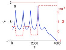
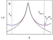
Figure 2: (color online) (a) A typical $\zeta$ solution (blue solid) when $\Delta\phi_{0}$ is in the fractal region, and the corresponding $M(\tau)$ curve (red dashed); (b) plots of the perturbed solution $\zeta(\tau)$ (blue solid), the unperturbed solution (red dashed), as well as the separatrix solution (black dash-dotted) from the $n$-th saddle approach to the next.

To motivate our analysis, we first illustrate in Fig. 2(a) a typical $\zeta$ solution when the initial condition lies in the sensitive region of Fig. 1. We see that $\zeta$ undergoes several large oscillations, then escapes to $-\infty$. Each oscillation corresponds to a “bounce” in the two-wave interactions. These bouncing sequences are the key to the existence of fractal structures, similar to other physical systems Campbell ; anninos ; Kivshar_Fei ; YangTan ; Dmitriev . Each local minimum of $\zeta$ will be called a saddle approach Goodman_Haberman . The corresponding $M(\tau)$ curve is also plotted in Fig. 2(a). We see that $M$ changes very little near a saddle approach, but changes significantly near maxima of $\zeta$. Below we will calculate the change in $M$ from one saddle approach to another. It turns out the $M$ formula will be coupled to $E$ and $F$, thus we need to calculate the changes in $E,M$ and $F$ simultaneously. To carry out these calculations, we notice two facts. One is that from one saddle approach to the next, the perturbed and unperturbed (i.e. integrable) solutions remain close to each other since $\varepsilon\ll 1$. The other fact is that at each saddle approach, $E_{n},M_{n}\ll 1$. This is so since initial $E_{0},M_{0}$ are always small for weak wave interactions, and they will remain small when $\varepsilon\ll 1$. To simplify our analysis, we also assume that at each saddle approach, $M_{n}/E_{n}\ll 1$. This assumption is satisfied for many initial conditions such as (3).

Now we calculate $E,M$ and $F$ from the $n$-th saddle approach to the next. From Eqs. (4) and (6), we get

$$\Delta M_{n}=\int^{\tau_{n+1}}_{\tau_{n}}\frac{dM}{d\tau}d\tau=\int^{\tau_{n+1}}_{\tau_{n}}\varepsilon e^{\zeta}\sin{\psi}\dot{\zeta}d\tau.$$ (12)

In view of the first fact above, the perturbed orbit in the above formula can be approximated by the integrable orbit [see Fig. 2(b)]. Due to the second fact, we can further approximate the integrable orbit by a separatrix orbit. Notice that the separatrix orbit (9) has three parameters. To select the appropriate parameters in the separatrix, we note that most contributions to the integral of (12) come from the $\zeta$-maximum region, thus it is natural to ask the separatrix solution to have the same $\zeta$-maximum point as the integrable solution [see Fig. 2(b)]. Then in view of Eq. (8), the above requirement selects $\sigma$ and $A$ in the separatrix (9) as

$$\sigma_{n}=\mbox{sgn}\left\{\mbox{Im}\left[-2C_{n}\textrm{\mbox{coth}}(C_{n}(\tau^{*}_{u}+F_{n}))\right]\right\};$$ (13)

$$A_{n}=2\left|C^{2}_{n}\textrm{csch}^{2}\left[C_{n}(\tau^{*}_{u}+F_{n})\right]\right|.$$ (14)

Here $\tau_{n}+\tau^{*}_{u}$ is the time the unperturbed solution $\zeta_{u}$ reaches the maximum. Due to the assumption $M_{n}/E_{n}\ll 1$, the unperturbed solution (to leading order) is a periodic solution with period $T_{p}=\sqrt{2}\pi/\sqrt{|E_{n}|}$. Thus $\tau^{*}_{u}=T_{p}/2$, and $\tau_{n+1}=\tau_{n}+T_{p}$. Utilizing the above results and noticing $T_{p}\gg 1$, Eq. (12) is asymptotically approximated by

$$\Delta M_{n}=\varepsilon\int^{+\infty}_{-\infty}e^{\zeta_{s}}\sin{\psi_{s}}\dot{\zeta}_{s}d\tau=\sigma_{n}\varepsilon\pi A_{n}/2.$$ (15)

By similar calculations and utilizing the symmetry properties of the separatrix solution (9), we find that

$$\Delta E_{n}=\varepsilon\int^{+\infty}_{-\infty}e^{\zeta_{s}}\sin{\psi_{s}}\dot{\psi}_{s}d\tau=0.$$ (16)

To calculate $F_{n+1}$, notice from Eqs. (4) and (7) that $F$ satisfies a linear inhomogeneous ODE:

$$\frac{dF}{d\tau}=-\frac{\dot{E}+i\dot{M}}{2(E+iM)}F+D,$$ (17)

where $D$ is a function of $(\zeta,\psi)$ whose expression is easy to obtain. The homogeneous solution of this ODE is $C^{-1}(\tau)$. Thus by using the method of variation of parameters, we can integrate the inhomogeneous ODE (17) from $\tau_{n}$ to $\tau_{n+1}$ and get

$$F_{n+1}=F_{n}\frac{C_{n}}{C_{n+1}}+\frac{\int^{\tau_{n+1}}_{\tau_{n}}\sqrt{E+iM}Dd\tau}{\sqrt{E_{n+1}+iM_{n+1}}}.$$ (18)

Due to the second fact of $E_{n},M_{n}\ll 1$, we can approximate the solution $(\zeta,\psi)$ in $D$ by the separatrix solution (9). Then to leading order in $\varepsilon$, we get

$$F_{n+1}=F_{n}\frac{C_{n}}{C_{n+1}}+\frac{\left.(\hat{\tau}+i\alpha)\sqrt{E+iM}\right|^{\tau_{n+1}}_{\tau_{n}}}{\sqrt{E_{n+1}+iM_{n+1}}}.$$ (19)

Here $\hat{\tau}=\tau-\tau_{n}-T_{p}/2$, and $\alpha=\sqrt{2}\sigma_{n}A_{n}^{-1/2}$.

Iteration equation (19) is quite complicated. Below, we simplify it. From Eq. (16), we get $E_{n}=E_{0}$. Under our assumption of $M_{n}/E_{n}\ll 1$, to leading order, Eq. (19) becomes

$$F_{n+1}=\frac{\pi}{\sqrt{2|E_{0}|}}+(F_{n}+\frac{\pi}{\sqrt{2|E_{0}|}})(1-\frac{M_{n+1}-M_{n}}{2E_{0}}i).$$ (20)

At the initial saddle approach, we find from Eq. (7) that $\mbox{Re}(F_{0})=-\pi/\sqrt{2|E_{0}|}$. Then solving Eq. (20), we get

$$F_{n}=\pi(2|E_{0}|)^{-1/2}\left[2n-1-i\hskip 0.56917ptS_{n}M_{n}/2E_{0}\right],$$ (21)

where $S_{n+1}M_{n+1}=2nM_{n+1}-(2n-S_{n})M_{n}$. Now we introduce a new variable $Q_{n}$:

$$Q_{n}-2nM_{n}=-S_{n}M_{n}=-(2|E_{0}|)^{3/2}\mbox{Im}[F_{n}]/\pi.$$ (22)

Then substituting formula (21) into (13), (14), keeping only their leading order terms in $M_{n}/E_{n}$, and putting the resulting expressions into (15), we obtain the simplified iteration equations as

$$M_{n+1}=M_{n}-\mbox{sgn}(Q_{n})8|E_{0}|^{3}\varepsilon/\pi Q_{n}^{2},$$ (23)

$$Q_{n+1}=Q_{n}+2M_{n+1}.$$ (24)

These equations are derived asymptotically near the separatrix orbit (9), and will be called the separatrix map. This map can be further normalized. Let

$$G=8|E_{0}|^{3}\varepsilon/\pi,\;\tilde{M}_{n}=G^{-1/3}M_{n},\;\tilde{Q}_{n}=G^{-1/3}Q_{n},$$ (25)

then the normalized separatrix map is

$$\tilde{M}_{n+1}=\tilde{M}_{n}-\frac{\mbox{sgn}(\varepsilon\tilde{Q}_{n})}{\tilde{Q}_{n}^{2}},$$ (26)

$$\tilde{Q}_{n+1}=\tilde{Q}_{n}+2\tilde{M}_{n+1}.\hskip 14.22636pt$$ (27)

This is a simple but important second-order area-preserving map, and it does not have any parameters in it (except a sign of $\varepsilon$). This universal map governs weak two-wave interactions in generalized NLS equations (1).

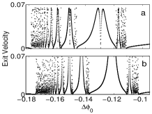
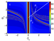
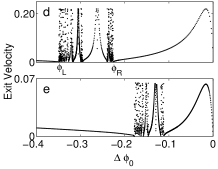
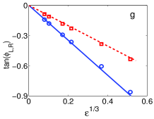
Figure 3: (color online) (a,b) The exit-velocity versus initial-phase-difference graphs from (a) PDE simulations and (b) map predictions; (c) the map’s $|\tilde{M}_{\infty}|$ graph in the $(\tilde{Q}_{0},\tilde{M}_{0})$ plane; (d,e) exit-velocity versus initial-phase-difference graphs of the PDE for $\varepsilon=0.01$ and $0.001$ respectively; (f) plots of the accumulation points $\phi_{L}$ and $\phi_{R}$ versus $\varepsilon$ from PDE simulations (circles and squares) and map predictions (solid and dashed lines).

Now we compare this map’s predictions with direct PDE simulations. Here we take the cubic-quintic nonlinearity in (2) with $\gamma$ and initial conditions as for Fig. 1(a). For the map, we iterate it to infinity to get $\tilde{M}_{\infty}$ (in practice, 500 iterations performed), which in turn gives $|\dot{\zeta}_{\infty}|$ from formula (11). With the variable scalings (5) and (25) considered, the exit velocity graph predicted from the map (26)-(27) is shown in Fig. 3(b), while that from the PDE simulations is shown in Fig. 3(a). Comparing these two graphs, it is clear that the map gives a good replication of the PDE’s fractal structure both qualitatively and quantitatively.

The separatrix map (26)-(27) exhibits a fractal structure in the graph of $|\tilde{M}_{\infty}|$ as a function of initial values $(\tilde{Q_{0}},\tilde{M_{0}})$, which is displayed in Fig. 3(c) (with $\mbox{sgn}(\varepsilon)=1$). This fractal of the map completely determines the fractal structures in the PDEs (1). For instance, for initial conditions (3), the corresponding initial values of the map are

$$\tilde{Q}_{0}=\tilde{M}_{0}=-2^{-1}(\pi/\varepsilon)^{1/3}\tan(\Delta\phi_{0}).$$ (28)

As $\Delta\phi_{0}$ varies, Eq. (28) gives a parameterized curve in the $(\tilde{Q}_{0},\tilde{M}_{0})$ plane, which is the white straight line in Fig.3 (c). This line cuts cross the fractal of the map in Fig. 3(c), and the intersection is precisely the fractal structure as observed in Fig. 1 for the PDE [see also Fig. 3(a,b)]. The scaling laws for fractals of the PDEs can be readily derived from Eq. (28) and Fig. 3(c). Let $P_{1}$ and $P_{2}$ denote the two accumulation points of the map’s fractal, which are $(\tilde{Q}_{0},\tilde{M}_{0})=(1.271,1.271)$ and $(0.741,0.741)$ as marked in Fig. 3(c). The corresponding accumulation points $\phi_{R}$ and $\phi_{L}$ in the fractal structures of the PDEs are marked in Fig. 3(d). Here $\phi_{L}$ and $\phi_{R}$ are the left and right ends of the fractal region. Then according to scalings (28), we find that $\phi_{R}=-\mbox{atan}(1.482\varepsilon^{1/3}/\pi^{1/3})$, and $\phi_{L}=-\mbox{atan}(2.542\varepsilon^{1/3}/\pi^{1/3})$. Hence the map analytically predicts that the fractal region of the PDE shrinks to $\Delta\phi_{0}=0$ as $\varepsilon\to 0$, and its shrinking speed is proportional to $\varepsilon^{1/3}$ for $\varepsilon\ll 1$. This is precisely what happens. To illustrate, we choose two $\gamma$ values 0.0029 and 0.0003 in Eq. (2), which correspond to $\varepsilon=0.01$ and $0.001$ respectively. The fractal structures of the PDEs for these $\gamma$ values are displayed in Fig. 3(d,e). It is seen that the fractal region indeed shrinks as $\varepsilon$ decreases. We further recorded the $\phi_{L}$ and $\phi_{R}$ values in the PDE fractals at a number of $\varepsilon$ values, and the data is plotted in Fig. 3(f). The theoretical formulae of $\phi_{L}$ and $\phi_{R}$ above are also plotted for comparison. It is seen that the PDE values and the map’s analytical predictions agree perfectly, confirming the asymptotic accuracy of the map (26)-(27).

In summary, we have asymptotically analyzed weak solitary wave interactions in the generalized nonlinear Schrödinger equations and obtained a simple universal map. This map gives a complete analytical characterization of universal fractal structures in these wave interactions. We expect that this work will stimulate research in other physical systems where weak solitary wave interactions arise, such as nonlinear optics, water waves and Bose-Einstein condensates.

References

- (1) M.J. Ablowitz and H. Segur, Solitons and the Inverse Scattering Transform, SIAM, Philadelphia, 1981.
- (2) A. Hasegawa and Y. Kodama, Solitons in Optical Communications, Clarendon, Oxford, 1995.
- (3) Y. Kivshar and G. Agrawal, Optical Solitons, Academic Press, San Diego, 2003.
- (4) V. I. Karpman and V. V. Solov’ev, Physica D 3, 142 (1981); K.A. Gorshkov and L.A. Ostrovsky, Physica D 3, 428 (1981).
- (5) D.K. Campbell, J.S. Schonfeld, and C.A. Wingate, Physica D 9, 1 (1983); M. Peyrard and D.K. Campbell, Physica D 9, 33 (1983).
- (6) P. Anninos, S. Oliveira, and R. A. Matzner, Phys. Rev. D 44, 1147 (1991).
- (7) Y. S. Kivshar, Z. Fei, and L. Vázquez, Phys. Rev. Lett. 67, 1177 (1991); Z. Fei, Y. S. Kivshar, and L. Váquez, Phys. Rev. A 45, 6019 (1992).
- (8) J. Yang and Y. Tan, Phys. Rev. Lett. 85, 3624 (2000); Y. Tan and J. Yang, Phys. Rev. E. 64, 056616 (2001).
- (9) S.V. Dmitriev, Yu.S. Kivshar, and T. Shigenari, Phys. Rev. E 64, 056613 (2001); S.V. Dmitriev and T. Shigenari, Chaos 12, 324 (2002).
- (10) Y. Zhu and J. Yang, Phys. Rev. E, 75, 036605 (2007).
- (11) R. H. Goodman and R. Haberman, SIAM J. Appl. Dyn. Sys. 4, 1195 (2005); R. H. Goodman and R. Haberman, Phys. Rev. Lett. 98, 104103 (2007).