Distributed Sensor Localization in Random Environments using Minimal Number of Anchor Nodes

Usman A. Khan, Soummya Kar, and José M. F. Moura
Department of Electrical and Computer Engineering
Carnegie Mellon University, 5000 Forbes Ave, Pittsburgh, PA 15213
{ukhan, moura}@ece.cmu.edu, soummyak@andrew.cmu.edu
Ph: (412)268-7103 Fax: (412)268-3890
All authors contributed equally to the paper. This work was partially supported by the DARPA DSO Advanced Computing and Mathematics Program Integrated Sensing and Processing (ISP) Initiative under ARO grant # DAAD 19-02-1-0180, by NSF under grants # ECS-0225449 and # CNS-0428404, by ONR under grant # MURI-N000140710747, and by an IBM Faculty Award.
Abstract

The paper develops DILOC, a distributive, iterative algorithm that locates M𝑀M sensors in m,m1superscript𝑚𝑚1\mathbb{R}^{m},m\geq 1, with respect to a minimal number of m+1𝑚1m+1 anchors with known locations. The sensors exchange data with their neighbors only; no centralized data processing or communication occurs, nor is there centralized knowledge about the sensors’ locations. DILOC uses the barycentric coordinates of a sensor with respect to its neighbors that are computed using the Cayley-Menger determinants. These are the determinants of matrices of inter-sensor distances. We show convergence of DILOC by associating with it an absorbing Markov chain whose absorbing states are the anchors. We introduce a stochastic approximation version extending DILOC to random environments when the knowledge about the intercommunications among sensors and the inter-sensor distances are noisy, and the communication links among neighbors fail at random times. We show a.s. convergence of the modified DILOC and characterize the error between the final estimates and the true values of the sensors’ locations. Numerical studies illustrate DILOC under a variety of deterministic and random operating conditions.

Keywords: Distributed iterative sensor localization; sensor networks; Cayley-Menger determinant; barycentric coordinates; absorbing Markov chain; stochastic approximation.

I Introduction

Localization is a fundamental problem in sensor networks. Information about the location of the sensors is key to process the sensors’ measurements accurately. In applications where sensors are deployed randomly, they have no knowledge of their exact locations, but equipping each of them with a localization device like a GPS is expensive, not robust to jamming in military applications, and is usually of limited use in indoor environments. Our goal is to develop a distributed (decentralized) localization algorithm where the sensors find their locations under a limited set of assumptions and conditions. To be more specific, we are motivated by applications where N=M+m+1𝑁𝑀𝑚1N=M+m+1 sensors in msuperscript𝑚\mathbb{R}^{m} (for example, m=2𝑚2m=2 corresponds to sensors lying on a plane, while for m=3𝑚3m=3 the sensors are in three dimensional Euclidean space) are deployed in a large geographical region. We assume that the deployment region lies in the convex hull of a small, in fact minimal, number of m+1𝑚1m+1 anchors, (m+1)Mmuch-less-than𝑚1𝑀(m+1)\ll M. The anchors know their locations. In such situations, the large geographical distances to the anchors makes it highly impractical for the M𝑀M non-anchor sensors to communicate directly with the anchors. Further, to compute the locations of the non-anchor sensors at a central station is not feasible when M𝑀M is large, as it requires large communication effort, expensive large-scale computation, and adds latency and bottlenecks to the network operation. These networks call for efficient distributed algorithms where each sensor communicates directly only with a few neighboring nodes (either sensors or anchors) and a low order computation is performed locally at the sensor and at each iteration of the algorithm, for example, see [1]. In this paper, we present a Distributed Iterative LOCalization algorithm (DILOC, pronounced die-lock) that overcomes the above challenges in large-scale randomly deployed networks.

In DILOC, the sensors start with an initial estimate of their locations, for example, a random guess. This random guess is arbitrary and does not need to place the sensors in the convex hull of the anchors. The sensors then update their locations, which we call the state of the network, by exchanging their state information only with a carefully chosen subset of m+1𝑚1m+1 of their neighbors. This state updating is a convex combination of the states of the neighboring nodes. The coefficients of the convex combination are the barycentric coordinates [2, 3] and are determined from the mutual inter-sensor distances among the sensors using the Cayley-Menger determinants. At each sensor l𝑙l its neighborhood set contains m+1𝑚1m+1 sensors, for example, its closest m+1𝑚1m+1 sensors, such that sensor l𝑙l lies in the convex hull of these m+1𝑚1m+1 neighbors. These neighbors may or may not include the anchors.

DILOC is distributed and iterative; each sensor updates locally its own state and then sends its state information to its neighbors; nowhere does DILOC need a fusion center or global communication. We prove almost sure (a.s.) convergence of DILOC in both deterministic and random network environments by showing that DILOC behaves as an absorbing Markov chain, where the anchors are the absorbing states. We prove convergence under a broad characterization of noise. In particular, we consider three types of randomness, acting simultaneously. These model many practical random sensing and communication distortions as, for example, when: (i) the inter-sensor distances are known up to random errors, which is common in cluttered environments and also in ad-hoc environments, where cheap low resolution sensors are deployed; (ii) the communication links between the sensors fail at random times. This is mainly motivated by wireless digital communication, where packets may get dropped randomly at each iteration, particularly, if the sensors are power limited or there are bandwidth or rate communication constraints in the network; and (iii) the communication among two sensors, when their communication link is active, is corrupted by noise.

Although a sensor can only communicate directly with its neighbors (e.g., sensors within a small radius), we assume that, when the links are deterministic and never fail, the network graph is connected, i.e., there is a communication path (by multihop) between any arbitrary pair of sensors. In a random environment, inter-sensor communication links may not stay active all the time and are subject to random failures. Consequently, there may be iterations when the network is not connected; actually, there might never be iterations when the network is connected. We will show under broad conditions almost sure convergence of an extended version of DILOC that we term as Distributed Localization in Random Environments (DLRE). DLRE employs stochastic approximation techniques using a decreasing weight sequence in the iterations.

In the following, we contrast our work with the existing literature on sensor localization.

Brief review of the literature: The literature on localization algorithms may be broadly characterized into centralized and distributed algorithms. Illustrative centralized localization algorithms include: maximum likelihood estimators that are formulated when the data is known to be described by a statistical model, [4, 5]; multi-dimensional scaling (MDS) algorithms that formulate the localization problem as a least squares problem at a centralized location, [6, 7]; work that exploits the geometry of the Euclidean space, like when locating a single robot using trilateration in m=3𝑚limit-from3m=3-dimensional space, see [8] where a geometric interpretation is given to the traditional algebraic distance constraint equations; localization algorithms with imprecise distance information, see [9] where the authors exploit the geometric relations among the distances in the optimization procedure; for additional work, see, e.g., [10, 11]. Centralized algorithms are fine in small or tethered network environments; but in large untethered networks, they incur high communication cost and may not be scalable; they depend on the availability and robustness of a central processor and have a single point of failure.

Distributed localization algorithms can be characterized into two classes: multilateration and successive refinements. In multilateration algorithms, [12, 13, 14, 15], each sensor estimates its range from the anchors and then calculates its location via multilateration, [16]. The multilateration scheme requires a high density of anchors, which is a practical limitation in large sensor networks. Further, the location estimates obtained from multilateration schemes are subject to large errors because the estimated sensor-anchor distance in large networks, where the anchors are far apart, is noisy. To overcome this problem, a high density of anchors is required. We, on the other hand, do not estimate distances to far-away nodes. Only local distances to nearby nodes are estimated that have better accuracy. This allows us to employ a minimal number of anchors.

A distributed multidimensional scaling algorithm is presented in [17]. Successive refinement algorithms that perform an iterative minimization of a cost function are presented in [18, 19, 20]. Reference [18] discusses an iterative scheme where they assume 5%percent55\% of the nodes as anchors. Reference [20] discusses a Self-Positioning Algorithm (SPA) that provides a GPS-free positioning and builds a relative coordinate system.

Another formulation to solve localization problems in a distributed fashion is the probabilistic approach. Nonparametric belief propagation on graphical models is used in [21]. Sequential Monte Carlo methods for mobile localization are considered in [22]. Particle filtering methods have been addressed in [23] where each sensor stores representative particles for its location that are weighted according to their likelihood. Reference [24] tracks and locates mobile robots using such probabilistic methods.

Completion of partially specified distance matrices is considered in [25, 26]. The approach is relevant when the (entire) partially specified distance matrix is available at a central location. The algorithms complete the unspecified distances under the geometrical constraints of the underlying network. The key point to note in our work is that our algorithm is distributed. In particular, it does not require a centralized location to perform the computations.

In comparison with these references, our algorithm, DILOC, is equivalent to solving in a distributed and iterative fashion a large system of linear algebraic equations where the system matrix is highly sparse. Our method exploits the structure of this matrix, which results from the topology of the communication graph of the network. We prove the a.s. convergence of the algorithm under broad noise conditions and characterize the bias and mean square error properties of the estimates of the sensor locations obtained by DILOC.

We divide the rest of the paper into two parts. The first part of the paper is concerned with the deterministic formulation of the localization problem and consists of sections IIIV. Section II presents preliminaries and then DILOC, the distributed iterative localization algorithm, that is based on barycentric coordinates, generalized volumes, and Cayley-Menger determinants. Section III proves DILOC’s convergence. Section IV presents the DILOC-REL, DILOC with relaxation, and proves that it asymptotically reduces to the deterministic case without relaxation. The second part of the paper consists of sections VVI and considers distributed localization in random noisy environments. Section V characterizes the random noisy environments and the iterative algorithm for these conditions. Section VI proves the convergence of the distributed localization algorithm in the noisy case that relies on a result on the convergence of Markov processes. Finally, we present detailed numerical simulations in Section VII and conclude the paper in Section VIII. Appendices AC provide a necessary test, the Cayley-Menger determinant and background material on absorbing Markov chains.

II Distributed Sensor Localization: DILOC

In this section, we formally state DILOC (distributed iterative localization algorithm) in m𝑚m-dimension Euclidean space, m(m1)superscript𝑚𝑚1\mathbb{R}^{m}~{}(m\geq 1), and introduce the necessary notation. Of course, for sensor localization, m=1𝑚1m=1 (sensors in a straight line), m=2𝑚2m=2 (plane), or m=3𝑚3m=3 (333d-space.) The generic case of m>3𝑚3m>3 is of interest, for example, when the graph nodes represent m𝑚m-dimensional feature vectors in classification problems, and the goal is still to find in a distributed fashion their global coordinates (with respect to a reference frame.) Since our results are general, we deal with m𝑚m-dimensional ‘localization,’ but, for easier reference, the reader may consider m=2𝑚2m=2 or m=3𝑚3m=3. To provide a quantitative assessment on some of the assumptions underlying DILOC, we will, when needed, assume that the deployment of the sensors in a given region follows a Poisson distribution. This random deployment is often assumed and is realistic; we use it to derive probabilistic bounds on the deployment density of the sensors and on the communication radius at each sensor; these can be straight forwardly related to the values of network field parameters (like transmitting power or signal-to-noise ratio) in order to implement DILOC. We discuss the computation/communication complexity of the algorithm and provide a simplistic, yet insightful, example that illustrates DILOC.

II-A Preliminaries and Notation

Recall that the sensors are in msuperscript𝑚\mathbb{R}^{m}. Let ΘΘ\Theta be the set of sensors or nodes in the network decomposed as

Θ=κΩ,Θ𝜅Ω\Theta=\kappa\cup\Omega, (1)

where κ𝜅\kappa is the set of anchors, i.e., the sensors whose locations are known, and ΩΩ\Omega is the set of sensors whose locations are to be determined. By |||\cdot| we mean the cardinality of the set, and we let |Θ|=NΘ𝑁\left|\Theta\right|=N, |κ|=m+1𝜅𝑚1\left|\kappa\right|=m+1, and |Ω|=MΩ𝑀\left|\Omega\right|=M. For a set ΨΨ\Psi of sensors, we denote its convex hull by 𝒞(Ψ)𝒞Ψ\mathcal{C}\left(\Psi\right)111The convex hull, 𝒞(Ψ)𝒞Ψ\mathcal{C}\left(\Psi\right), of a set of points in ΨΨ\Psi is the minimal convex set containing ΨΨ\Psi.. For example, if ΨΨ\Psi is a set of three non-coplanar sensors in a plane, then 𝒞(Ψ)𝒞Ψ\mathcal{C}\left(\Psi\right) is a triangle. We now define a few additional sets needed.

Let dlksubscript𝑑𝑙𝑘d_{lk} be the Euclidean distance between two sensors l,kΘ𝑙𝑘Θl,k\in\Theta. We associate with the sensor lΩ𝑙Ωl\in\Omega, a positive real number, rl>0subscript𝑟𝑙0r_{l}>0, and two sets 𝒦(l,rl)𝒦𝑙subscript𝑟𝑙\mathcal{K}\left(l,r_{l}\right) and Θl(rl)subscriptΘ𝑙subscript𝑟𝑙\Theta_{l}\left(r_{l}\right):

𝒦(l,rl)={kΘ:dlk<rl},𝒦𝑙subscript𝑟𝑙conditional-set𝑘Θsubscript𝑑𝑙𝑘subscript𝑟𝑙\displaystyle\mathcal{K}\left(l,r_{l}\right)=\left\{k\in\Theta:\>\>d_{lk}<r_{l}\right\}, (2)
Θl(rl)𝒦(l,rl),lΘl(rl),l𝒞(Θl(rl)),|Θl(rl)|=m+1,AΘl(rl)0,formulae-sequencesubscriptΘ𝑙subscript𝑟𝑙𝒦𝑙subscript𝑟𝑙formulae-sequence𝑙subscriptΘ𝑙subscript𝑟𝑙formulae-sequence𝑙𝒞subscriptΘ𝑙subscript𝑟𝑙formulae-sequencesubscriptΘ𝑙subscript𝑟𝑙𝑚1subscript𝐴subscriptΘ𝑙subscript𝑟𝑙0\displaystyle\Theta_{l}\left(r_{l}\right)\subseteq\mathcal{K}\left(l,r_{l}\right),\>\>l\notin\Theta_{l}\left(r_{l}\right),\>\>l\in\mathcal{C}\left(\Theta_{l}\left(r_{l}\right)\right),\>\>\left|\Theta_{l}\left(r_{l}\right)\right|=m+1,\>\>A_{\Theta_{l}\left(r_{l}\right)}\neq 0, (3)

where AΘl(rl)subscript𝐴subscriptΘ𝑙subscript𝑟𝑙A_{\Theta_{l}\left(r_{l}\right)} is the generalized volume (area in m=2𝑚2m=2-d, volume in m=3𝑚3m=3, and their generalization in higher dimensions) of 𝒞(Θl(rl))𝒞subscriptΘ𝑙subscript𝑟𝑙\mathcal{C}\left(\Theta_{l}\left(r_{l}\right)\right). The set 𝒦(l,rl)𝒦𝑙subscript𝑟𝑙\mathcal{K}\left(l,r_{l}\right) groups the neighboring sensors of l𝑙l within a radius rlsubscript𝑟𝑙r_{l} and, by (3), Θl(rl)subscriptΘ𝑙subscript𝑟𝑙\Theta_{l}\left(r_{l}\right), which we will often represent simply as ΘlsubscriptΘ𝑙\Theta_{l}, assuming rlsubscript𝑟𝑙r_{l} is understood from the context, is a subset of m+1𝑚1m+1 sensors such that sensor l𝑙l lies in its convex hull but is not one of its elements. In appendix A, we provide a procedure to test the convex hull inclusion of a sensor, i.e., for any sensor, l𝑙l, to determine if it lies in the convex hull of m+1𝑚1m+1 nodes arbitrarily chosen from the set, 𝒦(l,rl)𝒦𝑙subscript𝑟𝑙\mathcal{K}\left(l,r_{l}\right), of its neighbors. Finding such a set ΘlsubscriptΘ𝑙\Theta_{l} is an important step in DILOC and we refer to it as triangulation and ΘlsubscriptΘ𝑙\Theta_{l} is referred to as a triangulation set.

Let 𝐜lsubscript𝐜𝑙\mathbf{c}_{l} be the m𝑚m-dimensional coordinates for a node, lΘ𝑙Θl\in\Theta, with respect to a global coordinate system, written as the m𝑚m-dimensional row vector,

𝐜lsubscript𝐜𝑙\displaystyle\mathbf{c}_{l} =\displaystyle= [cl,1,cl,2,,cl,m].subscript𝑐𝑙1subscript𝑐𝑙2subscript𝑐𝑙𝑚\displaystyle\left[c_{l,1},c_{l,2},\ldots,c_{l,m}\right]. (4)

The true (possibly unknown) location of sensor l𝑙l is represented by 𝐜lsuperscriptsubscript𝐜𝑙\mathbf{c}_{l}^{\ast}. Because the distributed localization algorithm DILOC is iterative, 𝐜l(t)subscript𝐜𝑙𝑡\mathbf{c}_{l}(t) will represent the location vector, or state, for sensor l𝑙l at iteration t𝑡t.

Barycentric coordinates. DILOC is expressed in terms of the barycentric coordinates, alksubscript𝑎𝑙𝑘a_{lk}, of a sensor, lΩ𝑙Ωl\in\Omega, with respect to the nodes, kΘl𝑘subscriptΘ𝑙k\in\Theta_{l}, see [2, 3]. The barycentric coordinates, alksubscript𝑎𝑙𝑘a_{lk}, are unique and are given by

alk=A{l}Θl{k}AΘl,subscript𝑎𝑙𝑘subscript𝐴𝑙subscriptΘ𝑙𝑘subscript𝐴subscriptΘ𝑙a_{lk}=\dfrac{A_{\{l\}\cup\Theta_{l}\setminus\{k\}}}{A_{\Theta_{l}}}, (5)

with AΘl0subscript𝐴subscriptΘ𝑙0A_{\Theta_{l}}\neq 0, where ‘\setminus’ denotes the set difference, A{l}Θl{k}subscript𝐴𝑙subscriptΘ𝑙𝑘A_{\{l\}\cup\Theta_{l}\setminus\{k\}} is the generalized volume of the set {l}Θl{k}𝑙subscriptΘ𝑙𝑘\{l\}\cup\Theta_{l}\setminus\{k\}, i.e., the set ΘlsubscriptΘ𝑙\Theta_{l} with sensor l𝑙l added and node k𝑘k removed. The barycentric coordinates can be computed from the inter-sensor distances dlksubscript𝑑𝑙𝑘d_{lk} using the Cayley-Menger determinants as shown in appendix B. From (5), and the facts that the generalized volumes are non-negative and

kΘlAΘl{l}{k}=AΘl,l𝒞(Θl),formulae-sequencesubscript𝑘subscriptΘ𝑙subscript𝐴subscriptΘ𝑙𝑙𝑘subscript𝐴subscriptΘ𝑙𝑙𝒞subscriptΘ𝑙\sum_{k\in\Theta_{l}}A_{\Theta_{l}\cup\{l\}\setminus\{k\}}=A_{\Theta_{l}},\qquad l\in\mathcal{C}(\Theta_{l}), (6)

it follows that, for each lΩ𝑙Ωl\in\Omega, kΘl𝑘subscriptΘ𝑙k\in\Theta_{l},

alk[0,1],kΘlalk=1.formulae-sequencesubscript𝑎𝑙𝑘01subscript𝑘subscriptΘ𝑙subscript𝑎𝑙𝑘1a_{lk}\in[0,~{}1],\qquad\sum_{k\in\Theta_{l}}a_{lk}=1. (7)

II-B Distributed iterative localization algorithm.

Before presenting DILOC, we state explicitly state our assumptions.

(B0) Nondegeneracy. The generalized volume for κ𝜅\kappa, Aκ0subscript𝐴𝜅0A_{\kappa}\neq 0.222Nondegeneracy simply states that the anchors do not lie on a hyperplane. If this was the case, then the localization problem reduces to a lower dimensional problem, i.e., m1superscript𝑚1\mathbb{R}^{m-1} instead of msuperscript𝑚\mathbb{R}^{m}. For instance, if all the anchors in a network lie on a plane in 3superscript3\mathbb{R}^{3}, the localization problem can be thought of as localization in 2superscript2\mathbb{R}^{2}.

(B1) Anchor nodes. The anchors’ locations are known, i.e., their state remains constant

𝐜q(t)=𝐜q,qκ,t0.formulae-sequencesubscript𝐜𝑞𝑡superscriptsubscript𝐜𝑞formulae-sequence𝑞𝜅𝑡0\mathbf{c}_{q}(t)=\mathbf{c}_{q}^{\ast},\qquad q\in\kappa,\>t\geq 0. (8)

(B2) Convexity. All the sensors lie inside the convex hull of the anchors

𝒞(Ω)𝒞(κ).𝒞Ω𝒞𝜅\mathcal{C}(\Omega)\subset\mathcal{C}(\kappa). (9)

From (B2), the next Lemma follows easily.

Lemma 1 (Triangulation)

For every lΩ𝑙Ωl\in\Omega, there exist rl>0subscript𝑟𝑙0r_{l}>0 and Θl(rl)subscriptΘ𝑙subscript𝑟𝑙\Theta_{l}\left(r_{l}\right) with |Θl(rl)|=m+1subscriptΘ𝑙subscript𝑟𝑙𝑚1\left|\Theta_{l}\left(r_{l}\right)\right|=m+1 satisfying the properties in (3).

Proof.

Clearly, by (B2), κ𝜅\kappa satisfies (3) and the diameter of the network, maxl,kdlk,(lΩ,kκ)subscript𝑙𝑘subscript𝑑𝑙𝑘formulae-sequence𝑙Ω𝑘𝜅\max_{l,k}d_{lk},(l\in\Omega,k\in\kappa), could be taken as rlsubscript𝑟𝑙r_{l}. ∎

Lemma 1 provides an existence proof, but in localization in wireless sensor networks, it is important to triangulate a sensor not with the network diameter but with a small rlsubscript𝑟𝑙r_{l}. In fact, Section II-E discusses the probability of finding one such ΘlsubscriptΘ𝑙\Theta_{l} with rlmaxl,kdlk,(lΩ,kκ)much-less-thansubscript𝑟𝑙subscript𝑙𝑘subscript𝑑𝑙𝑘formulae-sequence𝑙Ω𝑘𝜅r_{l}\ll\max_{l,k}d_{lk},(l\in\Omega,k\in\kappa).

As a note, it is easily verified that every pair of sensors in 𝒞(Θl(rl))𝒞subscriptΘ𝑙subscript𝑟𝑙\mathcal{C}\left(\Theta_{l}\left(r_{l}\right)\right) is within a distance Rl=2rlsubscript𝑅𝑙2subscript𝑟𝑙R_{l}=2r_{l}. Think of m=2𝑚2m=2, then |Θl(rl)|=3subscriptΘ𝑙subscript𝑟𝑙3\left|\Theta_{l}\left(r_{l}\right)\right|=3, 𝒞(Θl(rl))𝒞subscriptΘ𝑙subscript𝑟𝑙\mathcal{C}\left(\Theta_{l}\left(r_{l}\right)\right) is a triangle and if rlsubscript𝑟𝑙r_{l} is the maximum distance of any interior point l𝑙l to the vertices of the triangle, the maximum distance between the 4 points (triangle vertices and l𝑙l) is 2rl2subscript𝑟𝑙2r_{l}. We complete stating the assumptions underlying DILOC.

(B3) inter-sensor distances. For lΩ𝑙Ωl\in\Omega, there exists at least an rl>0subscript𝑟𝑙0r_{l}>0 and Θl(rl)𝒦(l,rl)subscriptΘ𝑙subscript𝑟𝑙𝒦𝑙subscript𝑟𝑙\Theta_{l}\left(r_{l}\right)\subset\mathcal{K}\left(l,r_{l}\right), satisfying (3), such that l𝑙l has a communication link for every kΘl(rl)𝑘subscriptΘ𝑙subscript𝑟𝑙k\in\Theta_{l}\left(r_{l}\right) and knows the mutual distances among all the nodes in {l}Θl(rl)𝑙subscriptΘ𝑙subscript𝑟𝑙\{l\}\cup\Theta_{l}\left(r_{l}\right).

We can now present DILOC. There are two steps: a set-up phase and then DILOC proper. We discuss each separately.

DILOC set-up: Triangulation. In the set-up phase, each sensor l𝑙l triangulates itself, so that by the end of this phase we have paired every lΩ𝑙Ωl\in\Omega with its corresponding m+1𝑚1m+1 neighbors in ΘlsubscriptΘ𝑙\Theta_{l}. Since triangulation should be with a small rlsubscript𝑟𝑙r_{l}, the following is a practical protocol for the set-up phase. A sensor starts with a small communication radius, rlsubscript𝑟𝑙r_{l}, and chooses arbitrarily m+1𝑚1m+1 sensors within rlsubscript𝑟𝑙r_{l} and tests if it lies in the convex hull of these sensors using the procedure described in Appendix A. The sensor attempts this with all collections of m+1𝑚1m+1 sensors within rlsubscript𝑟𝑙r_{l}. If all attempts fail, the sensor adaptively increases, in small increments, its communication radius, rlsubscript𝑟𝑙r_{l}, and repeats the process. By (B2) and (9), success is eventually achieved and each sensor is triangulated by finding ΘlsubscriptΘ𝑙\Theta_{l} with properties (3) and (B3). If the sensors have directionality a much simpler algorithm based on Lemma 2 below, see also discussion following the Lemma, triangulates the sensor with high probability of success in one shot. To assess the practical implications required by DILOC’s set-up phase, Subsection II-E considers the realistic scenario where the sensors are deployed using a random Poisson distribution and computes in terms of deployment parameters the probability of finding at least one such ΘlsubscriptΘ𝑙\Theta_{l} in a given radius, rlsubscript𝑟𝑙r_{l}.

DILOC iterations: state updating. Once the set-up phase is complete; at time t+1𝑡1t+1, each sensor lΩ𝑙Ωl\in\Omega, iteratively updates its state, i.e., its current location estimate, by a convex combination of the states at time t𝑡t of the nodes in ΘlsubscriptΘ𝑙\Theta_{l}. The anchors do not update their state, since they know their locations. The updating is explicitly given by

𝐜l(t+1)={𝐜l(t),lκ,kΘlalk𝐜k(t),lΩ,subscript𝐜𝑙𝑡1casessubscript𝐜𝑙𝑡𝑙𝜅subscript𝑘subscriptΘ𝑙subscript𝑎𝑙𝑘subscript𝐜𝑘𝑡𝑙Ω\mathbf{c}_{l}(t+1)=\left\{\begin{array}[]{cc}\mathbf{c}_{l}(t),&l\in\kappa,\\ \sum_{k\in\Theta_{l}}a_{lk}\mathbf{c}_{k}(t),&l\in\Omega,\end{array}\right. (10)

where alksubscript𝑎𝑙𝑘a_{lk} are the barycentric coordinates of l𝑙l with respect to kΘl𝑘subscriptΘ𝑙k\in\Theta_{l}. DILOC in (10) is distributed since (i) the update is implemented at each sensor independently; (ii) at sensor lΩ𝑙Ωl\in\Omega, the update of the state, 𝐜l(t+1)subscript𝐜𝑙𝑡1\mathbf{c}_{l}(t+1), is obtained from the states of its m+1𝑚1m+1 neighboring nodes in ΘlsubscriptΘ𝑙\Theta_{l}; and (iii) there is no central location and only local information is available.

DILOC: Matrix format. For compactness of notation, we write DILOC (10) in matrix form. Without loss of generality, we index the anchors in κ𝜅\kappa as 1,2,,m+112𝑚11,2,\ldots,m+1 and the sensors in ΩΩ\Omega as m+2,m+3,,m+1+M=N𝑚2𝑚3𝑚1𝑀𝑁m+2,m+3,\ldots,m+1+M=N. We now stack the (row vectors) states, 𝐜lsubscript𝐜𝑙\mathbf{c}_{l}, given in (4) for all the N𝑁N nodes in the network in the N×m𝑁𝑚N\times m-dimensional coordinate matrix

𝐂=[𝐜1T,,𝐜NT]T.𝐂superscriptdelimited-[]superscriptsubscript𝐜1𝑇superscriptsubscript𝐜𝑁𝑇𝑇\mathbf{C}=\left[\begin{array}[]{c}\mathbf{c}_{1}^{T},\ldots,\mathbf{c}_{N}^{T}\end{array}\right]^{T}. (11)

DILOC equations in (10), now become in compact matrix form

𝐂(t+1)=𝚼𝐂(t).𝐂𝑡1𝚼𝐂𝑡\mathbf{C}(t+1)=\mathbf{\mathbf{\Upsilon}}\mathbf{C}(t). (12)

The structure of the N×N𝑁𝑁N\times N iteration matrix 𝚼𝚼\mathbf{\Upsilon} becomes more apparent if we partition it as

𝚼=[𝐈m+1𝟎𝐁𝐏],𝚼delimited-[]subscript𝐈𝑚10𝐁𝐏\mathbf{\Upsilon}=\left[\begin{array}[]{cc}\mathbf{I}_{m+1}&\mathbf{0}\\ \mathbf{B}&\mathbf{P}\end{array}\right], (13)

The first m+1𝑚1m+1 rows correspond to the update equations for the anchors in κ𝜅\kappa. Since the states of the anchors are constant, see (B1) and (8), the first m+1𝑚1m+1 rows of 𝚼𝚼\mathbf{\Upsilon} are zero except for a 111 at their (q,q),qκ={1,,m+1}𝑞𝑞𝑞𝜅1𝑚1(q,q),q\in\kappa=\{1,\ldots,m+1\} location. In other words, these first m+1𝑚1m+1 rows are the (m+1)×N𝑚1𝑁(m+1)\times N block matrix [𝐈m+1|𝟎]delimited-[]conditionalsubscript𝐈𝑚10\left[\mathbf{I}_{m+1}|\mathbf{0}\right], i.e., the (m+1)×(m+1)𝑚1𝑚1(m+1)\times(m+1) identity matrix 𝐈m+1subscript𝐈𝑚1\mathbf{I}_{m+1} concatenated with the (m+1)×M𝑚1𝑀(m+1)\times M zero matrix, 𝟎0\mathbf{0}.

Each of the M𝑀M remaining rows in 𝚼𝚼\mathbf{\Upsilon}, indexed by lΩ={m+2,m+3,,N}𝑙Ω𝑚2𝑚3𝑁l\in\Omega=\{m+2,m+3,\ldots,N\}, have only m+1𝑚1m+1 non-zero elements corresponding to the nodes in the triangulation set, ΘlsubscriptΘ𝑙\Theta_{l}, of l𝑙l, and these non-zero elements are the barycentric coordinates, alksubscript𝑎𝑙𝑘a_{lk}, of sensor l𝑙l with respect to the nodes in ΘlsubscriptΘ𝑙\Theta_{l}. The M×(m+1)𝑀𝑚1M\times(m+1) block 𝐁={blj}𝐁subscript𝑏𝑙𝑗\mathbf{B}=\{b_{lj}\} is a zero matrix, except in those rows corresponding to the sensors in ΩΩ\Omega that have a direct link to anchors. The M×M𝑀𝑀M\times M block 𝐏={plj}𝐏subscript𝑝𝑙𝑗\mathbf{P}=\left\{p_{lj}\right\} is also a sparse matrix where the non-zero entries in row l𝑙l correspond to the non-anchor nodes in ΘlsubscriptΘ𝑙\Theta_{l}. The matrices 𝚼𝚼\mathbf{\Upsilon}, 𝐏𝐏\mathbf{P}, and 𝐁𝐁\mathbf{B} have important properties that will be used to prove the convergence of the distributed iterative algorithm DILOC in Sections III and IV.

Remark. Equation (12) writes DILOC in matrix format for compactness; it should not be confused with a centralized algorithm–it still is a distributed iterative algorithm. It is iterative, because each iteration through (12) simply updates the (matrix of) state(s) from 𝐂(t)𝐂𝑡\mathbf{C}(t) to 𝐂(t+1)𝐂𝑡1\mathbf{C}(t+1). It is distributed because each row equation updates the state of sensor l𝑙l from the states of the m+1𝑚1m+1 nodes in ΘlsubscriptΘ𝑙\Theta_{l}. In all, the iteration matrix, 𝚼𝚼\mathbf{\Upsilon}, is highly sparse having exactly (m+1)+M(m+1)𝑚1𝑀𝑚1(m+1)+M(m+1) non-zeros out of possible (m+1+M)2superscript𝑚1𝑀2(m+1+M)^{2} elements.

II-C Example

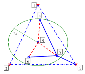
We consider an m=2𝑚2m=2-dimensional Euclidean plane with m+1=3𝑚13m+1=3 anchors and M=4𝑀4M=4 sensors, see Fig. 1.

Refer to caption
Figure 1: Deployment corresponding to the example in Section II-C.

The nodes are indexed such that the anchor set is κ={1,2,3},|κ|=m+1=3,formulae-sequence𝜅123𝜅𝑚13\kappa=\{1,2,3\},~{}|\kappa|=m+1=3, and the sensor set is Ω={4,5,6,7},|Ω|=M=4.formulae-sequenceΩ4567Ω𝑀4\Omega=\{4,5,6,7\},\,|\Omega|=M=4. The set of all the nodes in the network is, thus, Θ=κΩ={1,,7},|Θ|=N=7formulae-sequenceΘ𝜅Ω17Θ𝑁7\Theta=\kappa\cup\Omega=\{1,\ldots,7\},~{}|\Theta|=N=7. The triangulation set, Θl,lΩsubscriptΘ𝑙𝑙Ω\Theta_{l},~{}l\in\Omega, identified by using the convex hull inclusion test are Θ4={1,5,7},Θ5={4,6,7},Θ6={2,5,7},Θ7={3,4,6}.formulae-sequencesubscriptΘ4157formulae-sequencesubscriptΘ5467formulae-sequencesubscriptΘ6257subscriptΘ7346\Theta_{4}=\{1,5,7\},~{}\Theta_{5}=\{4,6,7\},~{}\Theta_{6}=\{2,5,7\},~{}\Theta_{7}=\{3,4,6\}. It is clear that these triangulation sets satisfy properties in (3). It can be verified that sensor 555 does not have any anchor node in its triangulation set, Θ5subscriptΘ5\Theta_{5}, and every other sensor has only one anchor in its respective triangulation set. Since, no sensor is able to communicate to m+1=3𝑚13m+1=3 anchors directly, no sensor can localize itself in a single step.

At each sensor, lΩ𝑙Ωl\in\Omega, the barycentric coordinates, alk,kΘlsubscript𝑎𝑙𝑘𝑘subscriptΘ𝑙a_{lk},~{}k\in\Theta_{l}, are computed using the inter-sensor distances (among the nodes in the set {l}Θl𝑙subscriptΘ𝑙\{l\}\cup\Theta_{l}) in the Cayley-Menger determinant. It is noteworthy that the inter-sensor distances that need to be known at each sensor l𝑙l to compute alksubscript𝑎𝑙𝑘a_{lk} are only the inter-sensor distances among the m+2𝑚2m+2 sensors in the set {l}Θl𝑙subscriptΘ𝑙\{l\}\cup\Theta_{l}. For instance, the distances in the Cayley-Menger determinant needed by sensor 555 to compute a54,a56,a57subscript𝑎54subscript𝑎56subscript𝑎57a_{54},a_{56},a_{57} are the inter-sensor distances among the nodes in the set, {5}Θ55subscriptΘ5\{5\}\cup\Theta_{5}, i.e., d54,d56,d57,d46,d47,d67subscript𝑑54subscript𝑑56subscript𝑑57subscript𝑑46subscript𝑑47subscript𝑑67d_{54},d_{56},d_{57},d_{46},d_{47},d_{67}. Due to (3) and the relation Θ5𝒦(l,r5)subscriptΘ5𝒦𝑙subscript𝑟5\Theta_{5}\subseteq\mathcal{K}(l,r_{5}), the nodes in {5}Θ55subscriptΘ5\{5\}\cup\Theta_{5} lie in a circle of radius, r5subscript𝑟5r_{5}, centered at sensor 555 (shown in Fig. 1); on the other hand, no two sensors in the set {5}Θ55subscriptΘ5\{5\}\cup\Theta_{5} can be more than R5=2r5subscript𝑅52subscript𝑟5R_{5}=2r_{5} apart. This justifies the choices of Rlsubscript𝑅𝑙R_{l} and rl=Rl/2subscript𝑟𝑙subscript𝑅𝑙2r_{l}=R_{l}/2 in (2).

Once the barycentric coordinates, alksubscript𝑎𝑙𝑘a_{lk}, are computed, DILOC for the sensors in ΩΩ\Omega is

𝐜l(t+1)subscript𝐜𝑙𝑡1\displaystyle\mathbf{c}_{l}(t+1) =\displaystyle= kΘlalk𝐜k(t),lΩ={4,5,6,7}.subscript𝑘subscriptΘ𝑙subscript𝑎𝑙𝑘subscript𝐜𝑘𝑡𝑙Ω4567\displaystyle\sum_{k\in\Theta_{l}}a_{lk}\mathbf{c}_{k}(t),\qquad l\in\Omega=\{4,5,6,7\}. (14)

In particular, for sensor 555, we have the following expression,

𝐜5(t+1)=a54𝐜4(t)+a56𝐜6(t)+a57𝐜7(t).subscript𝐜5𝑡1subscript𝑎54subscript𝐜4𝑡subscript𝑎56subscript𝐜6𝑡subscript𝑎57subscript𝐜7𝑡\mathbf{c}_{5}(t+1)=a_{54}\mathbf{c}_{4}(t)+a_{56}\mathbf{c}_{6}(t)+a_{57}\mathbf{c}_{7}(t).

DILOC for the anchors is given by

𝐜q(t)=𝐜q,qκ.formulae-sequencesubscript𝐜𝑞𝑡superscriptsubscript𝐜𝑞𝑞𝜅\mathbf{c}_{q}(t)=\mathbf{c}_{q}^{\ast},\qquad q\in\kappa.

We write DILOC for this example in the matrix format (12).

[𝐜1(t+1)𝐜2(t+1)𝐜3(t+1)𝐜4(t+1)𝐜5(t+1)𝐜6(t+1)𝐜7(t+1)]=[100000001000000010000a41000a450a47000a540a56a570a6200a650a6700a73a740a760][𝐜1(t)𝐜2(t)𝐜3(t)𝐜4(t)𝐜5(t)𝐜6(t)𝐜7(t)],delimited-[]subscript𝐜1𝑡1subscript𝐜2𝑡1subscript𝐜3𝑡1subscript𝐜4𝑡1subscript𝐜5𝑡1subscript𝐜6𝑡1subscript𝐜7𝑡1delimited-[]100000001000000010000subscript𝑎41000subscript𝑎450subscript𝑎47000subscript𝑎540subscript𝑎56subscript𝑎570subscript𝑎6200subscript𝑎650subscript𝑎6700subscript𝑎73subscript𝑎740subscript𝑎760delimited-[]subscript𝐜1𝑡subscript𝐜2𝑡subscript𝐜3𝑡subscript𝐜4𝑡subscript𝐜5𝑡subscript𝐜6𝑡subscript𝐜7𝑡\displaystyle\left[\begin{array}[]{c}\mathbf{c}_{1}(t+1)\\ \mathbf{c}_{2}(t+1)\\ \mathbf{c}_{3}(t+1)\\ \mathbf{c}_{4}(t+1)\\ \mathbf{c}_{5}(t+1)\\ \mathbf{c}_{6}(t+1)\\ \mathbf{c}_{7}(t+1)\\ \end{array}\right]=\left[\begin{array}[]{ccccccc}1&0&0&0&0&0&0\\ 0&1&0&0&0&0&0\\ 0&0&1&0&0&0&0\\ a_{41}&0&0&0&a_{45}&0&a_{47}\\ 0&0&0&a_{54}&0&a_{56}&a_{57}\\ 0&a_{62}&0&0&a_{65}&0&a_{67}\\ 0&0&a_{73}&a_{74}&0&a_{76}&0\\ \end{array}\right]\left[\begin{array}[]{c}\mathbf{c}_{1}(t)\\ \mathbf{c}_{2}(t)\\ \mathbf{c}_{3}(t)\\ \mathbf{c}_{4}(t)\\ \mathbf{c}_{5}(t)\\ \mathbf{c}_{6}(t)\\ \mathbf{c}_{7}(t)\\ \end{array}\right], (36)

where the initial condition are 𝐂(0)=[𝐜1,𝐜2,𝐜3,𝐜40,𝐜50,𝐜60,𝐜70]T𝐂0superscriptsuperscriptsubscript𝐜1superscriptsubscript𝐜2superscriptsubscript𝐜3superscriptsubscript𝐜40superscriptsubscript𝐜50superscriptsubscript𝐜60superscriptsubscript𝐜70𝑇\mathbf{C}(0)=[\mathbf{c}_{1}^{\ast},\mathbf{c}_{2}^{\ast},\mathbf{c}_{3}^{\ast},\mathbf{c}_{4}^{0},\mathbf{c}_{5}^{0},\mathbf{c}_{6}^{0},\mathbf{c}_{7}^{0}]^{T}, with 𝐜l0,lΩ,superscriptsubscript𝐜𝑙0𝑙Ω\mathbf{c}_{l}^{0},~{}l\in\Omega, being randomly chosen row vectors of appropriate dimensions.

Note here again that (36) is just a matrix representation of (14). DILOC is implemented in a distributed fashion as in (14). The matrix representation in (36) is included for compaction of notation and for the convergence analysis of the algorithm.

II-D Complexity of DILOC

Once the barycentric coordinates are computed, each sensor333By sensor, we usually mean a non-anchor node. performs the update in (10) that requires m+1𝑚1m+1 multiplications and m𝑚m additions. Assuming the computation complexity of the multiplication and the addition operations to be the same, the computation complexity of DILOC is 2m+12𝑚12m+1 operations, i.e., O(1)𝑂1O(1) per sensor, per iteration. Since each sensor exchanges information with m+1𝑚1m+1 nodes in its triangulation set, the communication complexity of DILOC is m+1𝑚1m+1 communications, i.e., O(1)𝑂1O(1) per sensor, per iteration. Hence, both the computation and communication complexity are O(M)𝑂𝑀O(M) for a network of M𝑀M sensors. Note that, since the triangulation set-up phase, which identifies Θl(rl)subscriptΘ𝑙subscript𝑟𝑙\Theta_{l}\left(r_{l}\right) and computes the barycentric coordinates, as explained in Subsection II-B, are to be carried out only once at the start of DILOC, they require a constant computation/communication complexity, so we do not account explicitly for it.

II-E Random Poisson Deployment

A common model in wireless sensor networks is the Poisson deployment [27, 28]. We illustrate it on the plane, m=2𝑚2m=2; the discussion can be extended to arbitrary dimensions. For a Poisson distribution with density, γ>0𝛾0\gamma>0, the mean number of sensors in a sector Q𝑄Q with area AQsubscript𝐴𝑄A_{Q} is γAQ𝛾subscript𝐴𝑄\gamma A_{Q}. The numbers of sensors in any two disjoint sectors, Q1subscript𝑄1Q_{1} and Q2subscript𝑄2Q_{2}, are independent random variables, and the locations of the sensors in a sector Q𝑄Q are uniformly distributed. We now characterize the probability of triangulating a sensor l𝑙l in a region of radius, rlsubscript𝑟𝑙r_{l}, centered at l𝑙l.

Refer to caption
Refer to caption
Figure 2: (a) Sensor l𝑙l identifies its triangulation set, ΘlsubscriptΘ𝑙\Theta_{l}, in the circle of radius, rlsubscript𝑟𝑙r_{l}, centered at sensor l𝑙l. The circle is divided into four disjoint sectors with equal areas, Q1,,Q4subscript𝑄1subscript𝑄4Q_{1},\ldots,Q_{4}. A sufficient condition for triangulation is that there exists at least one sensor in each of these four sectors. (b) Illustration of Lemma 2.

To this end, consider Fig. 2, which shows the triangulation region, a circle of radius, rlsubscript𝑟𝑙r_{l}, centered at sensor l𝑙l. Let Q1,Q2,Q3,Q4subscript𝑄1subscript𝑄2subscript𝑄3subscript𝑄4Q_{1},Q_{2},Q_{3},Q_{4} be four disjoint sectors partitioning this circle with equal areas, i.e., AQi=πrl24,i=1,,4formulae-sequencesubscript𝐴subscript𝑄𝑖𝜋superscriptsubscript𝑟𝑙24𝑖14A_{Q_{i}}=\dfrac{\pi r_{l}^{2}}{4},~{}i=1,\ldots,4.

Lemma 2

A sufficient condition to triangulate a sensor l2𝑙superscript2l\in\mathbb{R}^{2} is to have at least one sensor in each of the four disjoint equal area sectors, Qi,i=1,,4formulae-sequencesubscript𝑄𝑖𝑖14Q_{i},~{}i=1,\ldots,4, which partition the circle of radius of radius, rlsubscript𝑟𝑙r_{l}, centered at l𝑙l.

Proof.

In Fig. 2 consider the triangulation of sensor l𝑙l located at the center of the circle; we choose arbitrarily four sensors p1,p2,p3,p4subscript𝑝1subscript𝑝2subscript𝑝3subscript𝑝4p_{1},p_{2},p_{3},p_{4} in each of the four sectors Q1,Q2,Q3,Q4subscript𝑄1subscript𝑄2subscript𝑄3subscript𝑄4Q_{1},Q_{2},Q_{3},Q_{4}. Denote the polygon with vertices p1,p2,p3,p4subscript𝑝1subscript𝑝2subscript𝑝3subscript𝑝4p_{1},p_{2},p_{3},p_{4} by Pol(p1p2p3p4)Polsubscript𝑝1subscript𝑝2subscript𝑝3subscript𝑝4\mbox{Pol}\left(p_{1}p_{2}p_{3}p_{4}\right). Consider the diagonal444If Pol(p1p2p3p4)Polsubscript𝑝1subscript𝑝2subscript𝑝3subscript𝑝4\mbox{Pol}\left(p_{1}p_{2}p_{3}p_{4}\right) is concave, we choose the diagonal that lies inside Pol(p1p2p3p4)Polsubscript𝑝1subscript𝑝2subscript𝑝3subscript𝑝4\mbox{Pol}\left(p_{1}p_{2}p_{3}p_{4}\right), i.e., p1𝑝1p1p3𝑝3p3 in Fig. 2. If Pol(p1p2p3p4)Polsubscript𝑝1subscript𝑝2subscript𝑝3subscript𝑝4\mbox{Pol}\left(p_{1}p_{2}p_{3}p_{4}\right) is convex, we can choose any of the two diagonals and the proof follows. p1𝑝1p1p3𝑝3p3 that partitions this polygon into two triangles p1p2p3subscript𝑝1subscript𝑝2subscript𝑝3\triangle p_{1}p_{2}p_{3} and p1p3p4subscript𝑝1subscript𝑝3subscript𝑝4\triangle p_{1}p_{3}p_{4}. Since lPol(p1p2p3p4)𝑙Polsubscript𝑝1subscript𝑝2subscript𝑝3subscript𝑝4l\in\mbox{Pol}\left(p_{1}p_{2}p_{3}p_{4}\right) and p1p2p3p1p3p4=Pol(p1p2p3p4)subscript𝑝1subscript𝑝2subscript𝑝3subscript𝑝1subscript𝑝3subscript𝑝4Polsubscript𝑝1subscript𝑝2subscript𝑝3subscript𝑝4\triangle p_{1}p_{2}p_{3}\cup\triangle p_{1}p_{3}p_{4}=\mbox{Pol}\left(p_{1}p_{2}p_{3}p_{4}\right) with p1p2p3p1p3p4=subscript𝑝1subscript𝑝2subscript𝑝3subscript𝑝1subscript𝑝3subscript𝑝4\triangle p_{1}p_{2}p_{3}\cap\triangle p_{1}p_{3}p_{4}=\varnothing, then either lp1p2p3𝑙subscript𝑝1subscript𝑝2subscript𝑝3l\in\triangle p_{1}p_{2}p_{3} or lp1p3p4𝑙subscript𝑝1subscript𝑝3subscript𝑝4l\in\triangle p_{1}p_{3}p_{4}. The triangle in which l𝑙l lies becomes the triangulating set, ΘlsubscriptΘ𝑙\Theta_{l}, of l𝑙l.

This completes the proof. The generalization to higher dimensions is straightforward; for instance, in 3superscript3\mathbb{R}^{3}, we have eight sectors and an arbitrary sensor l𝑙l is triangulated with at least one sensor in each of these eight sectors (with equal volume) of a sphere of radius, rlsubscript𝑟𝑙r_{l}, centered around l𝑙l.∎

Let Q¯isubscript¯𝑄𝑖\overline{Q}_{i} be the set of sensors in the sector Qisubscript𝑄𝑖Q_{i}. It follows from the Poisson deployment that the probability of finding at least one sensor in a sector, Qisubscript𝑄𝑖Q_{i}, of area AQisubscript𝐴subscript𝑄𝑖A_{Q_{i}} is

(|Q¯i|>0)=(1expγAQi).subscript¯𝑄𝑖01superscript𝛾subscript𝐴subscript𝑄𝑖\mathbb{P}\left(|\overline{Q}_{i}|>0\right)=\left(1-\exp^{-\gamma A_{Q_{i}}}\right). (37)

Since the distribution of the number of sensors in disjoint sectors is independent, the probability of finding at least one sensor in each of the sets, Q¯1,,Q¯4subscript¯𝑄1subscript¯𝑄4\overline{Q}_{1},\ldots,\overline{Q}_{4}, is the product

(|Q¯i|>0,i)=(1expγπrl2/4)4.subscript¯𝑄𝑖0for-all𝑖superscript1superscript𝛾𝜋superscriptsubscript𝑟𝑙244\mathbb{P}\left(\left|\overline{Q}_{i}\right|>0,\,\forall\,i\right)=\left(1-\exp^{-\gamma\pi r_{l}^{2}/4}\right)^{4}. (38)

Thus, we have

Θl=(Θl exists satisfying (3))(|Q¯i|>0,i).subscriptsubscriptΘ𝑙subscriptΘ𝑙 exists satisfying (3)subscript¯𝑄𝑖0for-all𝑖\mathbb{P}_{\Theta_{l}}=\mathbb{P}\left(\Theta_{l}\mbox{ exists satisfying~{}\eqref{linC}}\right)\geq\mathbb{P}\left(|\overline{Q}_{i}|>0,~{}\forall~{}i\right). (39)

This shows that, for a given deployment density, γ𝛾\gamma, we can choose, rlsubscript𝑟𝑙r_{l}, appropriately, to guarantee the triangulation with arbitrarily high probability. Indeed, it follows from (39) that, for an arbitrary, 0<ϵ<10italic-ϵ10<\epsilon<1, to get the probability of triangulation to be greater than ϵitalic-ϵ\epsilon, i.e., ΘlϵsubscriptsubscriptΘ𝑙italic-ϵ\mathbb{P}_{\Theta_{l}}\geq\epsilon, the radius rlsubscript𝑟𝑙r_{l} should be

Rl2(4ln(1ϵ14)γπ)12,subscript𝑅𝑙2superscript4ln1superscriptitalic-ϵ14𝛾𝜋12R_{l}\geq 2\left(\dfrac{-4{\rm ln}\left(1-\epsilon^{\frac{1}{4}}\right)}{\gamma\pi}\right)^{\frac{1}{2}}, (40)

In alternative, if we are limited by the communication radius, Rlsubscript𝑅𝑙R_{l}, to guarantee ΘlϵsubscriptsubscriptΘ𝑙italic-ϵ\mathbb{P}_{\Theta_{l}}\geq\epsilon, we will need the deployment density, γ𝛾\gamma, to be larger than

γ4π(Rl/2)2ln(1ϵ14).𝛾4𝜋superscriptsubscript𝑅𝑙22ln1superscriptitalic-ϵ14\gamma\geq\dfrac{-4}{\pi\left(R_{l}/2\right)^{2}}{\rm ln}\left(1-\epsilon^{\frac{1}{4}}\right). (41)

For example, if the sensors are deployed (following a Poisson distribution) with a density of γ=1𝛾1\gamma=1 sensor//m2, then we can compute from equations (40)–(41) that 999999% of the sensors will be able to triangulate (identify ΘlsubscriptΘ𝑙\Theta_{l}) themselves if they can communicate to at least a radius of Rl=5.52subscript𝑅𝑙5.52R_{l}=5.52m. The remaining (1%percent11\%) of the sensors may require to communicate to a larger radius.

It also follows from the above discussion that if the sensors are equipped with a sense of directionality (for example, if they all have ultrasound transducers) then each sensor has to find one neighbor in each of its 444 sectors, Ql,1,Ql,2,Ql,3,Ql,4subscript𝑄𝑙1subscript𝑄𝑙2subscript𝑄𝑙3subscript𝑄𝑙4Q_{l,1},Q_{l,2},Q_{l,3},Q_{l,4} (in m=2𝑚2m=2-d space). Once a neighbor is found, triangulation chooses 333 out of these 444, in order to identify ΘlsubscriptΘ𝑙\Theta_{l}. The computational complexity in m=2𝑚2m=2-d Euclidean space is 4choose3=44choose344~{}\mbox{choose}~{}3=4. Without directionality the process of finding ΘlsubscriptΘ𝑙\Theta_{l} has the (expected) computation complexity of γπrl2choose3𝛾𝜋superscriptsubscript𝑟𝑙2choose3\gamma\pi r_{l}^{2}~{}\mbox{choose}~{}3.

III Convergence of DILOC

In this section, we prove the convergence of DILOC to the exact locations of the sensors, 𝐜l,lΩsuperscriptsubscript𝐜𝑙𝑙Ω\mathbf{c}_{l}^{\ast},~{}l\in\Omega. To formally state the convergence result, we provide briefly some background and additional results, based on assumptions (B0)(B3).

The entries of the rows of the iteration matrix 𝚼𝚼\mathbf{\Upsilon}, in (12), are either zero or the barycentric coordinates, alksubscript𝑎𝑙𝑘a_{lk}, which are positive, and, by (7), add to 1. This matrix can then be interpreted as the transition matrix of a Markov chain. We then describe localization problem and DILOC in terms of a Markov chain. Let the assumptions (B0)–(B3) in Section II-B hold and the N𝑁N nodes in the sensor network correspond to the states of a Markov chain where let the (ij𝑖𝑗ij)-th element of the iteration matrix, 𝚼={υij}𝚼subscript𝜐𝑖𝑗\mathbf{\Upsilon}=\{\upsilon_{ij}\} defines the probability that the i𝑖ith state goes to the j𝑗jth state. Because of the structure of 𝚼𝚼\mathbf{\Upsilon}, this chain is a very special Markov chain.

Absorbing Markov chain. Let an N×N𝑁𝑁N\times N matrix, 𝚼={υij}𝚼subscript𝜐𝑖𝑗\mathbf{\Upsilon}=\{\upsilon_{ij}\}, denote the transition probability matrix of a Markov chain with N𝑁N states, si,i=1,,Nsubscript𝑠formulae-sequence𝑖𝑖1𝑁s_{i,i=1,\ldots,N}. A state sisubscript𝑠𝑖s_{i} is called absorbing if the probability of leaving that state is 00 (i.e., υij=0,ijformulae-sequencesubscript𝜐𝑖𝑗0𝑖𝑗\upsilon_{ij}=0,i\neq j, in other words υii=1subscript𝜐𝑖𝑖1\upsilon_{ii}=1). A Markov chain is said to be absorbing if it has at least one absorbing state, and if from every state it is possible to go with non-zero probability to an absorbing state (not necessarily in one step). In an absorbing Markov chain, a state which is not absorbing is called transient. For additional background, see, for example, [29].

Lemma 3

The underlying Markov chain with the transition probability matrix given by the iteration matrix, 𝚼𝚼\mathbf{\Upsilon}, is absorbing.

Proof.

We prove by contradiction. Since υii=1,iκformulae-sequencesubscript𝜐𝑖𝑖1𝑖𝜅\upsilon_{ii}=1,~{}i\in\kappa, the anchors are the absorbing states of the Markov chain. Since υii=0,iΩformulae-sequencesubscript𝜐𝑖𝑖0𝑖Ω\upsilon_{ii}=0,i\in\Omega, the (non-anchor) sensors are the transient states. Partition the transient states into two clusters C1 and C2, such that each transient state in C1 can go with non-zero probability to at least one of the absorbing states and, with probability 1, the transient states in C2 cannot reach an absorbing states. It follows that with probability 1 the transient states in C2 cannot reach the transient states in C1 (in one or multiple steps); otherwise, they reach an absorbing state with a non-zero probability. Let’s consider the lie on the boundary of the convex hull, 𝒞(\mathcal{C}(C2))), i.e., the vertices of 𝒞(\mathcal{C}(C2))). Because they are on boundary, they cannot lie in the interior of the convex hull any subset of sensors in 𝒞(\mathcal{C}(C2))), and, thus, cannot triangulate themselves, which contradicts Lemma 1 and assumption (B3). In order to triangulate the boundary sensors in 𝒞(\mathcal{C}(C2))), the boundary sensors in C2 must be able to reach the transient states and/or the absorbing states, that is to say that the boundary sensors in 𝒞(\mathcal{C}(C2))) have to reach the sensors in C1 to be able to triangulate themselves. Hence, the Markov chain is absorbing. ∎

Consider the partitioning of the iteration matrix, 𝚼𝚼\mathbf{\Upsilon}, in (13). With the Markov chain interpretation, the M×(m+1)𝑀𝑚1M\times(m+1) block 𝐁={blj}𝐁subscript𝑏𝑙𝑗\mathbf{B}=\{b_{lj}\} is a transition probability matrix for the transient states to reach the absorbing states in one-step, and the block M×M𝑀𝑀M\times M 𝐏={plj}𝐏subscript𝑝𝑙𝑗\mathbf{P}=\{p_{lj}\} is a transition probability matrix for the transient states. With (13), 𝚼t+1superscript𝚼𝑡1\mathbf{\Upsilon}^{t+1} can be written as

𝚼t+1=[𝐈m+1𝟎k=0t𝐏k𝐁𝐏t+1],superscript𝚼𝑡1delimited-[]subscript𝐈𝑚10superscriptsubscript𝑘0𝑡superscript𝐏𝑘𝐁superscript𝐏𝑡1\mathbf{\Upsilon}^{t+1}=\left[\begin{array}[]{cc}\mathbf{I}_{m+1}&\mathbf{0}\\ \displaystyle\sum_{k=0}^{t}\mathbf{P}^{k}\mathbf{B}&\mathbf{P}^{t+1}\end{array}\right], (42)

and, as t𝑡t goes to infinity, we have

limt𝚼t+1=[𝐈m+1𝟎(𝐈M𝐏)1𝐁𝟎],subscript𝑡superscript𝚼𝑡1delimited-[]subscript𝐈𝑚10superscriptsubscript𝐈𝑀𝐏1𝐁0\lim_{t\rightarrow\infty}\mathbf{\Upsilon}^{t+1}=\left[\begin{array}[]{cc}\mathbf{I}_{m+1}&\mathbf{0}\\ \left(\mathbf{I}_{M}-\mathbf{P}\right)^{-1}\mathbf{B}&\mathbf{0}\end{array}\right], (43)

by Lemmas 5 and 6, in appendix C. Lemmas 5 and 6 use the fact that if 𝐏𝐏\mathbf{P} is the matrix associated to the transient states of an absorbing Markov chain, then ρ(𝐏)<1𝜌𝐏1\rho(\mathbf{P})<1, where ρ()𝜌\rho(\cdot) is the spectral radius of a matrix. With (43), DILOC (10) converges to

limt𝐂(t+1)=[𝐈m+1𝟎(𝐈M𝐏)1𝐁𝟎]𝐂(0).subscript𝑡𝐂𝑡1delimited-[]subscript𝐈𝑚10superscriptsubscript𝐈𝑀𝐏1𝐁0𝐂0\lim_{t\rightarrow\infty}\mathbf{C}(t+1)=\left[\begin{array}[]{cc}\mathbf{I}_{m+1}&\mathbf{0}\\ \left(\mathbf{I}_{M}-\mathbf{P}\right)^{-1}\mathbf{B}&\mathbf{0}\end{array}\right]\mathbf{C}(0). (44)

In (44), the coordinates of the M𝑀M sensors in ΩΩ\Omega (last M𝑀M rows of 𝐂(t+1)𝐂𝑡1\mathbf{C}(t+1)) are written as a function of the m+1𝑚1m+1 anchors in κ𝜅\kappa whose coordinates are exactly known. The limiting values of the states of the M𝑀M sensors in ΩΩ\Omega are written in terms of the coordinates of the m+1𝑚1m+1 anchors in κ𝜅\kappa weighted by (𝐈M𝐏)1𝐁superscriptsubscript𝐈𝑀𝐏1𝐁(\mathbf{I}_{M}-\mathbf{P})^{-1}\mathbf{B}. To show that the limiting values are indeed the exact solution, we give the following Lemma.

Lemma 4

Let 𝐜lsuperscriptsubscript𝐜𝑙\mathbf{c}_{l}^{\ast} be the exact coordinates of a node, lΘ𝑙Θl\in\Theta. Let the M×(m+1)𝑀𝑚1M\times(m+1) matrix, 𝐃={dlj},lΩ,jκformulae-sequence𝐃subscript𝑑𝑙𝑗formulae-sequence𝑙Ω𝑗𝜅\mathbf{D}=\{d_{lj}\},l\in\Omega,j\in\kappa, be the matrix of the barycentric coordinates of the M𝑀M sensors (in ΩΩ\Omega) in terms of the m+1𝑚1m+1 anchors in κ𝜅\kappa, relating the coordinates of the sensors to the coordinates of the anchors by

𝐜l=jκdlj𝐜j,lΩ.formulae-sequencesuperscriptsubscript𝐜𝑙subscript𝑗𝜅subscript𝑑𝑙𝑗superscriptsubscript𝐜𝑗𝑙Ω\mathbf{c}_{l}^{\ast}=\sum_{j\in\kappa}d_{lj}\mathbf{c}_{j}^{\ast},\qquad\qquad l\in\Omega. (45)

Then, we have

𝐃𝐃\displaystyle\mathbf{D} =\displaystyle= (𝐈M𝐏)1𝐁.superscriptsubscript𝐈𝑀𝐏1𝐁\displaystyle\left(\mathbf{I}_{M}-\mathbf{P}\right)^{-1}\mathbf{B}. (46)
Proof.

Clearly (𝐈M𝐏)subscript𝐈𝑀𝐏(\mathbf{I}_{M}-\mathbf{P}) is invertible, since, by (121) in Appendix C, ρ(𝐏)<1𝜌𝐏1\rho(\mathbf{P})<1; this follows from the fact that the eigenvalues of the matrix 𝐈M𝐏subscript𝐈𝑀𝐏\mathbf{I}_{M}-\mathbf{P} are 1λj1subscript𝜆𝑗1-\lambda_{j}, where λjsubscript𝜆𝑗\lambda_{j} is the j𝑗jth eigenvalue of the matrix 𝐏𝐏\mathbf{P} and |λj|<1,j=1,,Mformulae-sequencesubscript𝜆𝑗1for-all𝑗1𝑀|\lambda_{j}|<1,~{}\forall j=1,\ldots,M. It suffices to show that,

𝐃𝐃\displaystyle\mathbf{D} =\displaystyle= 𝐁+𝐏𝐃,𝐁𝐏𝐃\displaystyle\mathbf{B+PD}, (47)

since (46) follows from (47). In (47), 𝐃𝐃\mathbf{D} and 𝐁𝐁\mathbf{B} are both M×(m+1)𝑀𝑚1M\times(m+1) matrices, whereas 𝐏𝐏\mathbf{P} is an M×M𝑀𝑀M\times M matrix whose non-zero elements are the barycentric coordinates for the sensors in ΩΩ\Omega. Hence, for the lj𝑙𝑗lj-th element in (47), we need to show that

dlj=blj+kΩplkdkj.subscript𝑑𝑙𝑗subscript𝑏𝑙𝑗subscript𝑘Ωsubscript𝑝𝑙𝑘subscript𝑑𝑘𝑗d_{lj}=b_{lj}+\sum_{k\in\Omega}p_{lk}d_{kj}. (48)

For an arbitrary sensor, lΩ𝑙Ωl\in\Omega, its triangulation set, ΘlsubscriptΘ𝑙\Theta_{l}, may contain nodes from both κ𝜅\kappa and ΩΩ\Omega. We denote κΘlsubscript𝜅subscriptΘ𝑙\kappa_{\Theta_{l}} as the elements of ΘlsubscriptΘ𝑙\Theta_{l} that are anchors, and ΩΘlsubscriptΩsubscriptΘ𝑙\Omega_{\Theta_{l}} as the elements of ΘlsubscriptΘ𝑙\Theta_{l} that are non-anchor sensors. The exact coordinates, 𝐜lsuperscriptsubscript𝐜𝑙\mathbf{c}_{l}^{\ast}, of the sensor, l𝑙l, can be expressed as a convex combination of the coordinates of its neighbors in its triangulation set, kΘl𝑘subscriptΘ𝑙k\in\Theta_{l}, using the barycentric coordinates, alksubscript𝑎𝑙𝑘a_{lk}, i.e.,

𝐜lsuperscriptsubscript𝐜𝑙\displaystyle\mathbf{c}_{l}^{\ast} =\displaystyle= kΘlalk𝐜k,subscript𝑘subscriptΘ𝑙subscript𝑎𝑙𝑘superscriptsubscript𝐜𝑘\displaystyle\sum_{k\in\Theta_{l}}a_{lk}\mathbf{c}_{k}^{\ast}, (49)
=\displaystyle= jκΘlalj𝐜j+kΩΘlalk𝐜k,subscript𝑗subscript𝜅subscriptΘ𝑙subscript𝑎𝑙𝑗superscriptsubscript𝐜𝑗subscript𝑘subscriptΩsubscriptΘ𝑙subscript𝑎𝑙𝑘superscriptsubscript𝐜𝑘\displaystyle\sum_{j\in\kappa_{\Theta_{l}}}a_{lj}\mathbf{c}_{j}^{\ast}+\sum_{k\in\Omega_{\Theta_{l}}}a_{lk}\mathbf{c}_{k}^{\ast},
=\displaystyle= jκblj𝐜j+kΩplk𝐜k,subscript𝑗𝜅subscript𝑏𝑙𝑗superscriptsubscript𝐜𝑗subscript𝑘Ωsubscript𝑝𝑙𝑘superscriptsubscript𝐜𝑘\displaystyle\sum_{j\in\kappa}b_{lj}\mathbf{c}_{j}^{\ast}+\sum_{k\in\Omega}p_{lk}\mathbf{c}_{k}^{\ast},

since the scalars, aljsubscript𝑎𝑙𝑗a_{lj}, are given by

alj={blj,if jκΘl,plj,if jΩΘl,0,if jΘl.subscript𝑎𝑙𝑗casessubscript𝑏𝑙𝑗if 𝑗subscript𝜅subscriptΘ𝑙subscript𝑝𝑙𝑗if 𝑗subscriptΩsubscriptΘ𝑙0if 𝑗subscriptΘ𝑙\displaystyle a_{lj}=\left\{\begin{array}[]{cc}b_{lj},&\qquad\mbox{if }j\in\kappa_{\Theta_{l}},\\ p_{lj},&\qquad\mbox{if }j\in\Omega_{\Theta_{l}},\\ 0,&\qquad\mbox{if }j\notin\Theta_{l}.\end{array}\right. (53)

Equation (49) becomes, after writing each kΩ𝑘Ωk\in\Omega in terms of the m+1𝑚1m+1 anchors in κ𝜅\kappa,

𝐜lsuperscriptsubscript𝐜𝑙\displaystyle\mathbf{c}_{l}^{\ast} =\displaystyle= jκblj𝐜j+kΩplkjκdkj𝐜j,subscript𝑗𝜅subscript𝑏𝑙𝑗superscriptsubscript𝐜𝑗subscript𝑘Ωsubscript𝑝𝑙𝑘subscript𝑗𝜅subscript𝑑𝑘𝑗superscriptsubscript𝐜𝑗\displaystyle\sum_{j\in\kappa}b_{lj}\mathbf{c}_{j}^{\ast}+\sum_{k\in\Omega}p_{lk}\sum_{j\in\kappa}d_{kj}\mathbf{c}_{j}^{\ast}, (54)
=\displaystyle= jκblj𝐜j+jκkΩplkdkj𝐜j,subscript𝑗𝜅subscript𝑏𝑙𝑗superscriptsubscript𝐜𝑗subscript𝑗𝜅subscript𝑘Ωsubscript𝑝𝑙𝑘subscript𝑑𝑘𝑗superscriptsubscript𝐜𝑗\displaystyle\sum_{j\in\kappa}b_{lj}\mathbf{c}_{j}^{\ast}+\sum_{j\in\kappa}\sum_{k\in\Omega}p_{lk}d_{kj}\mathbf{c}_{j}^{\ast},
=\displaystyle= jκ(blj+kΩplkdkj)𝐜j.subscript𝑗𝜅subscript𝑏𝑙𝑗subscript𝑘Ωsubscript𝑝𝑙𝑘subscript𝑑𝑘𝑗superscriptsubscript𝐜𝑗\displaystyle\sum_{j\in\kappa}\left(b_{lj}+\sum_{k\in\Omega}p_{lk}d_{kj}\right)\mathbf{c}_{j}^{\ast}.

This is a representation of the coordinates of sensor, l𝑙l, in terms of the coordinates of the anchors, jκ𝑗𝜅j\in\kappa. Since for each jκ𝑗𝜅j\in\kappa, the value inside the parentheses is non-negative with their sum over jκ𝑗𝜅j\in\kappa being 1 and the fact that the barycentric representation is unique, we must have

dlj=blj+kΩplkdkj,subscript𝑑𝑙𝑗subscript𝑏𝑙𝑗subscript𝑘Ωsubscript𝑝𝑙𝑘subscript𝑑𝑘𝑗d_{lj}=b_{lj}+\sum_{k\in\Omega}p_{lk}d_{kj}, (55)

which, comparing to (45), completes the proof. ∎

We now recapitulate these results in the following theorem.

Theorem 1 (DILOC convergence)

DILOC (10) converges to the exact coordinates, 𝐜lsuperscriptsubscript𝐜𝑙\mathbf{c}_{l}^{\ast}, of the M𝑀M sensors (with unknown locations) in ΩΩ\Omega, i.e.,

limt𝐜l(t+1)=𝐜l,lΩ.formulae-sequencesubscript𝑡subscript𝐜𝑙𝑡1superscriptsubscript𝐜𝑙for-all𝑙Ω\lim_{t\rightarrow\infty}\mathbf{c}_{l}(t+1)=\mathbf{c}_{l}^{\ast},\qquad\forall~{}l\in\Omega. (56)
Proof.

The proof is a consequence of Lemmas 3 and 4. ∎

Convergence rate. The convergence rate of the localization algorithm depends on the spectral radius of the matrix 𝐏𝐏\mathbf{P}, which by (121) in Appendix C is strictly less than one. This is a consequence of the fact that 𝐏𝐏\mathbf{P} is a sub-stochastic matrix. The convergence is slow if the spectral radius, ρ(𝐏)𝜌𝐏\rho(\mathbf{P}), is close to 111. This can happen if the matrix 𝐁𝐁\mathbf{B} is close to a zero matrix, 𝟎0\mathbf{0}. This is the case if and only if the sensors cluster in a region of very small area inside the convex hull of the anchors, and the anchors themselves are very far apart. In fact, it can be seen that in this case the barycentric coordinates for the sensors with κΘlsubscript𝜅subscriptΘ𝑙\kappa_{\Theta_{l}}\neq\varnothing (see Lemma 4 for this notation) corresponding to the elements in κΘlsubscript𝜅subscriptΘ𝑙\kappa_{\Theta_{l}} are close to zero. Since in practical wireless sensor applications the sensors are assumed to be deployed in a geometric or a Poisson fashion (see details in Section II-E), the probability of this to happen is arbitrarily close to 00.

IV DILOC with Relaxation

In this Section, we modify DILOC to speed its convergence rate and to obtain a form that is more suitable to study distributed localization in random environments. We observe that in DILOC (10), at time t+1𝑡1t+1, the expression for 𝐜l(t+1),lΩsubscript𝐜𝑙𝑡1𝑙Ω\mathbf{c}_{l}(t+1),~{}l\in\Omega, does not involve its own coordinates, 𝐜l(t)subscript𝐜𝑙𝑡\mathbf{c}_{l}(t), at time t𝑡t. We introduce a relaxation parameter, α(0,1]𝛼01\alpha\in(0,1], in the iterations, such that, the expression of 𝐜l(t+1)subscript𝐜𝑙𝑡1\mathbf{c}_{l}(t+1) is a convex combination of 𝐜l(t)subscript𝐜𝑙𝑡\mathbf{c}_{l}(t) and (10). We refer to this version as the DILOC with relaxation, DILOC-REL. It is given by

𝐜l(t+1)subscript𝐜𝑙𝑡1\displaystyle\mathbf{c}_{l}(t+1) =\displaystyle= {(1α)𝐜l(t)+α𝐜l(t)=𝐜l(t),lκ,(1α)𝐜l(t)+αkΘlalk𝐜k(t),lΩ.cases1𝛼subscript𝐜𝑙𝑡𝛼subscript𝐜𝑙𝑡subscript𝐜𝑙𝑡𝑙𝜅1𝛼subscript𝐜𝑙𝑡𝛼subscript𝑘subscriptΘ𝑙subscript𝑎𝑙𝑘subscript𝐜𝑘𝑡𝑙Ω\displaystyle\left\{\begin{array}[]{cc}(1-\alpha)\mathbf{c}_{l}(t)+\alpha\mathbf{c}_{l}(t)=\mathbf{c}_{l}(t),&l\in\kappa,\\ (1-\alpha)\mathbf{c}_{l}(t)+\alpha\sum_{k\in\Theta_{l}}a_{lk}\mathbf{c}_{k}(t),&l\in\Omega.\end{array}\right. (59)

DILOC is the special case of DILOC-REL with α=1𝛼1\alpha=1. The matrix representation of DILOC-REL is

𝐂(t+1)=𝐇𝐂(t),𝐂𝑡1𝐇𝐂𝑡\mathbf{C}(t+1)=\mathbf{HC}(t), (60)

where 𝐇=(1α)𝐈N+α𝚼𝐇1𝛼subscript𝐈𝑁𝛼𝚼\mathbf{H}=\left(1-\alpha\right)\mathbf{I}_{N}+\alpha\mathbf{\Upsilon} and 𝐈Nsubscript𝐈𝑁\mathbf{I}_{N} is the N×N𝑁𝑁N\times N identity matrix. It is straightforward to show that the iteration matrix, 𝐇𝐇\mathbf{H}, corresponds to a transition probability matrix of an absorbing Markov chain, where the anchors are the absorbing states and the sensors are the transient states. Let 𝐉=(1α)𝐈M+α𝐏𝐉1𝛼subscript𝐈𝑀𝛼𝐏\mathbf{J}=\left(1-\alpha\right)\mathbf{I}_{M}+\alpha\mathbf{P}; partitioning 𝐇𝐇\mathbf{H} as

𝐇=[𝐈m+1𝟎α𝐁𝐉].𝐇delimited-[]subscript𝐈𝑚10𝛼𝐁𝐉\mathbf{H}=\left[\begin{array}[]{cc}\mathbf{I}_{m+1}&\mathbf{0}\\ \alpha\mathbf{B}&\mathbf{J}\end{array}\right]. (61)

We note the following

𝐇t+1=[𝐈m+1𝟎k=0t𝐉kα𝐁𝐉t+1],superscript𝐇𝑡1delimited-[]subscript𝐈𝑚10superscriptsubscript𝑘0𝑡superscript𝐉𝑘𝛼𝐁superscript𝐉𝑡1\mathbf{H}^{t+1}=\left[\begin{array}[]{cc}\mathbf{I}_{m+1}&\mathbf{0}\\ \displaystyle\sum_{k=0}^{t}\mathbf{J}^{k}\mathbf{\alpha B}&\mathbf{J}^{t+1}\end{array}\right], (62)

and, as t𝑡t\rightarrow\infty,

limt𝐇t+1=[𝐈m+1𝟎(𝐈M𝐉)1α𝐁𝟎],subscript𝑡superscript𝐇𝑡1delimited-[]subscript𝐈𝑚10superscriptsubscript𝐈𝑀𝐉1𝛼𝐁0\lim_{t\rightarrow\infty}\mathbf{H}^{t+1}=\left[\begin{array}[]{cc}\mathbf{I}_{m+1}&\mathbf{0}\\ \left(\mathbf{I}_{M}-\mathbf{J}\right)^{-1}\mathbf{\alpha B}&\mathbf{0}\end{array}\right], (63)

from Lemmas 5 and 6. Lemmas 5 and 6 apply to 𝐇𝐇\mathbf{H}, since 𝐇𝐇\mathbf{H} is non-negative and ρ(𝐉)<1𝜌𝐉1\rho(\mathbf{J})<1. To show ρ(𝐉)<1𝜌𝐉1\rho(\mathbf{J})<1, we recall that ρ(𝐏)<1𝜌𝐏1\rho(\mathbf{P})<1 and the eigenvalues of 𝐉𝐉\mathbf{J} are (1α)+αλj1𝛼𝛼subscript𝜆𝑗(1-\alpha)+\alpha\lambda_{j}, where λjsubscript𝜆𝑗\lambda_{j} are the eigenvalues of 𝐏𝐏\mathbf{P}. Therefore, we have

ρ(𝐉)𝜌𝐉\displaystyle\rho(\mathbf{J}) =\displaystyle= maxj|(1α)+αλj|<1.subscript𝑗1𝛼𝛼subscript𝜆𝑗1\displaystyle\max_{j}|(1-\alpha)+\alpha\lambda_{j}|<1. (64)

The following Theorem establishes convergence of DILOC-REL.

Theorem 2

DILOC-REL (59) converges to the exact coordinates, 𝐜lsuperscriptsubscript𝐜𝑙\mathbf{c}_{l}^{\ast}, of the M𝑀M sensors (with unknown locations) in ΩΩ\Omega, i.e.,

limt𝐜l(t+1)=𝐜l,lΩ.formulae-sequencesubscript𝑡subscript𝐜𝑙𝑡1superscriptsubscript𝐜𝑙for-all𝑙Ω\lim_{t\rightarrow\infty}\mathbf{c}_{l}(t+1)=\mathbf{c}_{l}^{\ast},\qquad\forall~{}l\in\Omega. (65)
Proof.

It suffices to show that

(𝐈M𝐉)1α𝐁=(𝐈M𝐏)1𝐁.superscriptsubscript𝐈𝑀𝐉1𝛼𝐁superscriptsubscript𝐈𝑀𝐏1𝐁\left(\mathbf{I}_{M}-\mathbf{J}\right)^{-1}\mathbf{\alpha B}=\left(\mathbf{I}_{M}-\mathbf{P}\right)^{-1}\mathbf{B}. (66)

To this end, we note that

(𝐈M𝐉)1α𝐁superscriptsubscript𝐈𝑀𝐉1𝛼𝐁\displaystyle\left(\mathbf{I}_{M}-\mathbf{J}\right)^{-1}\mathbf{\alpha B} =\displaystyle= (𝐈M((1α)𝐈M+α𝐏))1α𝐁,superscriptsubscript𝐈𝑀1𝛼subscript𝐈𝑀𝛼𝐏1𝛼𝐁\displaystyle\left(\mathbf{I}_{M}-\left(\left(1-\alpha\right)\mathbf{I}_{M}+\alpha\mathbf{P}\right)\right)^{-1}\mathbf{\alpha B}, (67)

which reduces to (66) after basic algebraic manipulations. The convergence of DILOC-REL thus follows from Lemma 4. ∎

As mentioned, the advantage of DILOC-REL is twofold: since ρ(𝐉)𝜌𝐉\rho(\mathbf{J}) is a function of α𝛼\alpha, we may optimize the convergence rate over α𝛼\alpha; and DILOC-REL forms the basis for the distributed localization algorithm in random environments (DLRE) that we discuss in Sections V and VI.

V Distributed Localization in Random Environments: Assumptions and Algorithm

This and the next Section study distributed iterative localization in more realistic practical scenarios, when the inter-sensor distances are known up to errors, the communication links between sensors may fail and, when alive, the communication among sensors is corrupted by noise. We write the update equations for DILOC-REL, (60), in terms of the columns, 𝐜j(t)superscript𝐜𝑗𝑡\mathbf{c}^{j}(t)1jm1𝑗𝑚1\leq j\leq m, of the coordinate matrix, 𝐂(t)𝐂𝑡\mathbf{C}(t). Column j𝑗j corresponds to the vector of the j𝑗j-th estimate coordinates of all the N𝑁N sensor locations555In the sequel, we omit the subscripts from the identity matrix, 𝐈𝐈\mathbf{I}, and its dimensions will be clear from the context.. The updates are

𝐜j(t+1)=[(1α)𝐈+α𝚼]𝐜j(t),1jm.formulae-sequencesuperscript𝐜𝑗𝑡1delimited-[]1𝛼𝐈𝛼𝚼superscript𝐜𝑗𝑡1𝑗𝑚\mathbf{c}^{j}(t+1)=\left[(1-\alpha)\mathbf{I}+\alpha\mathbf{\Upsilon}\right]\mathbf{c}^{j}(t),~{}1\leq j\leq m. (68)

We partition 𝐜j(t)superscript𝐜𝑗𝑡\mathbf{c}^{j}(t) as

𝐜j(t)=[𝐮j𝐱j(t)],superscript𝐜𝑗𝑡delimited-[]superscript𝐮𝑗missing-subexpressionsuperscript𝐱𝑗𝑡missing-subexpression\mathbf{c}^{j}(t)=\left[\begin{array}[]{ll}\mathbf{u}^{j}\\ \mathbf{x}^{j}(t)\end{array}\right], (69)

where, 𝐮j(m+1)×1superscript𝐮𝑗superscript𝑚11\mathbf{u}^{j}\in\mathbb{R}^{(m+1)\times 1} corresponds to the j𝑗j-th coordinates of the anchors, which are know (hence, we omit the time index, as they are not updated), and 𝐱j(t)M×1superscript𝐱𝑗𝑡superscript𝑀1\mathbf{x}^{j}(t)\in\mathbb{R}^{M\times 1} corresponds to the estimates of the j𝑗j-th coordinates of the non-anchor sensors, hence not known. Since, update is performed only on the 𝐱j(t)superscript𝐱𝑗𝑡\mathbf{x}^{j}(t), (68) is equivalent to the following recursion:

𝐱j(t+1)=[(1α)𝐈+α𝐏]𝐱j(t)+α𝐁𝐮j.superscript𝐱𝑗𝑡1delimited-[]1𝛼𝐈𝛼𝐏superscript𝐱𝑗𝑡𝛼superscript𝐁𝐮𝑗\mathbf{x}^{j}(t+1)=\left[(1-\alpha)\mathbf{I}+\alpha\mathbf{P}\right]\mathbf{x}^{j}(t)+\alpha\mathbf{B}\mathbf{u}^{j}. (70)

Thus, to implement the sequence of iterations in (70) perfectly, the l𝑙l-th sensor at iteration t𝑡t needs the corresponding rows of the matrices 𝐏𝐏\mathbf{P} and 𝐁𝐁\mathbf{B}, and, in addition, the current estimates,  cnj(t),nΘlsuperscriptsubscript𝑐𝑛𝑗𝑡𝑛subscriptΘ𝑙c_{n}^{j}(t),n\in\Theta_{l} (j𝑗j-th component of the n𝑛n-th sensor coordinates), of its neighbors’ positions. In practice, there are several limitations: (i) The computation of the matrices 𝐏𝐏\mathbf{P} and 𝐁𝐁\mathbf{B} requires inter-sensor distance computations, which are not perfect in a random environment; (ii) the communication channels, or links, between neighboring channels may fail at random times; and (iii) because of imperfect communication, each sensor receives only noisy versions of its neighbors current state. Hence, in a random environment, we need to modify the iteration sequence in (70) to account for the partial imperfect information received by a sensor at each iteration. We start by stating formally our modeling assumptions.

  • (C1) Randomness in system matrices. At each iteration, each sensor needs the corresponding row of the system matrices 𝐁𝐁\mathbf{B} and 𝐏𝐏\mathbf{P}, which in turn, depend on the inter-sensor distance measurements, which can be, possibly, random. Since a single measurement of the inter-sensor distances may lead to a large random noise, we assume the sensors estimate the required distances at each iteration of the algorithm (note that this leads to an implicit averaging of the unbiased noisy effects, as will be demonstrated later.) In other words, at each iteration, the l𝑙l-th sensor can only get estimates, 𝐁^l(t)subscript^𝐁𝑙𝑡\widehat{\mathbf{B}}_{l}(t) and 𝐏^l(t)subscript^𝐏𝑙𝑡\widehat{\mathbf{P}}_{l}(t), of the corresponding rows of the 𝐁𝐁\mathbf{B} and 𝐏𝐏\mathbf{P} matrices, respectively. In the generic imperfect communication case, we have

    𝐁^(t)=𝐁+𝐒𝐁+𝐒~𝐁(t)^𝐁𝑡𝐁subscript𝐒𝐁subscript~𝐒𝐁𝑡\widehat{\mathbf{B}}(t)=\mathbf{B}+\mathbf{S}_{\mathbf{B}}+\widetilde{\mathbf{S}}_{\mathbf{B}}(t) (71)

    where {𝐒~𝐁(t)}t0subscriptsubscript~𝐒𝐁𝑡𝑡0\left\{\widetilde{\mathbf{S}}_{\mathbf{B}}(t)\right\}_{t\geq 0} is an independent sequence of random matrices with,

    𝔼[𝐒~𝐁(t)]=0,t,supt0𝔼[𝐒~𝐁(t)2]=k𝐁<.formulae-sequence𝔼delimited-[]subscript~𝐒𝐁𝑡0for-all𝑡subscriptsupremum𝑡0𝔼delimited-[]superscriptnormsubscript~𝐒𝐁𝑡2subscript𝑘𝐁\mathbb{E}\left[\widetilde{\mathbf{S}}_{\mathbf{B}}(t)\right]=0,\>\forall t,\>\>\sup_{t\geq 0}\mathbb{E}\left[\left\|\widetilde{\mathbf{S}}_{\mathbf{B}}(t)\right\|^{2}\right]=k_{\mathbf{B}}<\infty. (72)

    Here, 𝐒𝐁subscript𝐒𝐁\mathbf{S}_{\mathbf{B}} is the mean measurement error. Similarly, for 𝐏𝐏\mathbf{P}, we have

    𝐏^(t)=𝐏+𝐒𝐏+𝐒~𝐏(t),^𝐏𝑡𝐏subscript𝐒𝐏subscript~𝐒𝐏𝑡\widehat{\mathbf{P}}(t)=\mathbf{P}+\mathbf{S}_{\mathbf{P}}+\widetilde{\mathbf{S}}_{\mathbf{P}}(t), (73)

    where {𝐒~𝐏(t)}t0subscriptsubscript~𝐒𝐏𝑡𝑡0\left\{\widetilde{\mathbf{S}}_{\mathbf{P}}(t)\right\}_{t\geq 0} is an independent sequence of random matrices with,

    𝔼[𝐒~𝐏(t)]=0,t,supt0𝔼[𝐒~𝐏(t)2]=k𝐏<.formulae-sequence𝔼delimited-[]subscript~𝐒𝐏𝑡0for-all𝑡subscriptsupremum𝑡0𝔼delimited-[]superscriptnormsubscript~𝐒𝐏𝑡2subscript𝑘𝐏\mathbb{E}\left[\widetilde{\mathbf{S}}_{\mathbf{P}}(t)\right]=0,\>\forall t,\>\>\sup_{t\geq 0}\mathbb{E}\left[\left\|\widetilde{\mathbf{S}}_{\mathbf{P}}(t)\right\|^{2}\right]=k_{\mathbf{P}}<\infty. (74)

    Likewise, 𝐒𝐏subscript𝐒𝐏\mathbf{S}_{\mathbf{P}} is the mean measurement error. Note that this way of writing B~(t),P~(t)~𝐵𝑡~𝑃𝑡\widetilde{B}(t),\widetilde{P}(t) does not require the noise model to be additive. It only says that any random object may be written as the sum of a deterministic mean part and the corresponding zero mean random part. The moment assumptions in eqns. (72,74) are very weak and, in particular, are satisfied if the sequences {𝐁^(t)}t0subscript^𝐁𝑡𝑡0\left\{\widehat{\mathbf{B}}(t)\right\}_{t\geq 0} and  {𝐏^(t)}t0subscript^𝐏𝑡𝑡0\left\{\widehat{\mathbf{P}}(t)\right\}_{t\geq 0} are i.i.d. with finite variance.

  • (C2) Random Link Failure: We assume that the inter-sensor communication links fail randomly. This happens, for example, in wireless sensor network applications, where occasionally data packets are dropped. To this end, if the sensors l𝑙l and n𝑛n share a communication link (or, nΘl𝑛subscriptΘ𝑙n\in\Theta_{l}), we assume that the link fails with some probability 1qln1subscript𝑞𝑙𝑛1-q_{ln} at each iteration, where 0<qln10subscript𝑞𝑙𝑛10<q_{ln}\leq 1. We associate with each such potential network link, a binary random variable, eln(t)subscript𝑒𝑙𝑛𝑡e_{ln}(t), where eln(t)=1subscript𝑒𝑙𝑛𝑡1e_{ln}(t)=1 indicates that the corresponding network link is active at time t𝑡t, whereas eln(t)=0subscript𝑒𝑙𝑛𝑡0e_{ln}(t)=0 indicates a link failure. Note that 𝔼[eln]=qln𝔼delimited-[]subscript𝑒𝑙𝑛subscript𝑞𝑙𝑛\mathbb{E}\left[e_{ln}\right]=q_{ln}.

  • (C3) Additive Channel Noise: Let {vlnj(t)}l,n,j,tsubscriptsuperscriptsubscript𝑣𝑙𝑛𝑗𝑡𝑙𝑛𝑗𝑡\left\{v_{ln}^{j}(t)\right\}_{l,n,j,t} be a family of independent zero mean random variables such that

    supl,n,j,t𝔼[vlnj(t)]2=kv<.subscriptsupremum𝑙𝑛𝑗𝑡𝔼superscriptdelimited-[]superscriptsubscript𝑣𝑙𝑛𝑗𝑡2subscript𝑘𝑣\sup_{l,n,j,t}\mathbb{E}\left[v_{ln}^{j}(t)\right]^{2}=k_{v}<\infty. (75)

    We assume that, at the t𝑡t-th iteration, if the network link  (l,n)𝑙𝑛(l,n) is active, sensor l𝑙l receives only a corrupt version,  ylnj(t)superscriptsubscript𝑦𝑙𝑛𝑗𝑡y_{ln}^{j}(t), of sensor n𝑛n’s state, cnj(t)superscriptsubscript𝑐𝑛𝑗𝑡c_{n}^{j}(t), given by

    ylnj(t)=cnj(t)+vlnj(t).superscriptsubscript𝑦𝑙𝑛𝑗𝑡superscriptsubscript𝑐𝑛𝑗𝑡superscriptsubscript𝑣𝑙𝑛𝑗𝑡y_{ln}^{j}(t)=c_{n}^{j}(t)+v_{ln}^{j}(t). (76)

    This models the channel noise. The moment assumption in eqn. (75) is very weak and holds, in particular, if the channel noise is i.i.d.

  • (C4) Independence: We assume that the sequences,  {𝐒~𝐁(t),𝐒~𝐏(t)}t0subscriptsubscript~𝐒𝐁𝑡subscript~𝐒𝐏𝑡𝑡0\left\{\widetilde{\mathbf{S}}_{\mathbf{B}}(t),\widetilde{\mathbf{S}}_{\mathbf{P}}(t)\right\}_{t\geq 0},  {eln(t)}l,n,tsubscriptsubscript𝑒𝑙𝑛𝑡𝑙𝑛𝑡\left\{e_{ln}(t)\right\}_{l,n,t}, and {vlnj(t)}l,n,j,tsubscriptsuperscriptsubscript𝑣𝑙𝑛𝑗𝑡𝑙𝑛𝑗𝑡\left\{v_{ln}^{j}(t)\right\}_{l,n,j,t} are mutually independent. These assumptions do not put restrictions on the distributional form of the random errors, only that they obey some weak moment conditions.

Clearly, under the random environment model (as detailed in Assumptions (C1)-(C4), the algorithm in (70) is not appropriate to update the sensors states. We now consider the following state update recursion for the random environment case.

Distributed Localization in Random Environment Algorithm (DLRE):

xlj(t+1)superscriptsubscript𝑥𝑙𝑗𝑡1\displaystyle x_{l}^{j}(t+1) =\displaystyle= (1α(t))xlj(t)+α(t)[nκΘleln(t)𝐁^ln(t)qln(unj+vlnj(t))]1𝛼𝑡superscriptsubscript𝑥𝑙𝑗𝑡𝛼𝑡delimited-[]subscript𝑛𝜅subscriptΘ𝑙subscript𝑒𝑙𝑛𝑡subscript^𝐁𝑙𝑛𝑡subscript𝑞𝑙𝑛superscriptsubscript𝑢𝑛𝑗superscriptsubscript𝑣𝑙𝑛𝑗𝑡\displaystyle\left(1-\alpha\left(t\right)\right)x_{l}^{j}(t)+\alpha(t)\left[\sum_{n\in\kappa\cap\Theta_{l}}\frac{e_{ln}(t)\widehat{\mathbf{B}}_{ln}(t)}{q_{ln}}\left(u_{n}^{j}+v_{ln}^{j}(t)\right)\right]
+\displaystyle+ α(t)[nΩΘleln(t)𝐏^ln(t)qln(xnj(t)+vlnj(t))],lΩ,  1jmformulae-sequence𝛼𝑡delimited-[]subscript𝑛ΩsubscriptΘ𝑙subscript𝑒𝑙𝑛𝑡subscript^𝐏𝑙𝑛𝑡subscript𝑞𝑙𝑛superscriptsubscript𝑥𝑛𝑗𝑡superscriptsubscript𝑣𝑙𝑛𝑗𝑡𝑙Ω1𝑗𝑚\displaystyle\alpha(t)\left[\sum_{n\in\Omega\cap\Theta_{l}}\frac{e_{ln}(t)\widehat{\mathbf{P}}_{ln}(t)}{q_{ln}}\left(x_{n}^{j}(t)+v_{ln}^{j}(t)\right)\right],\>\>l\in\Omega,\,\,1\leq j\leq m

In contrast with DILOC-REL, in (V), the gain α(t)𝛼𝑡\alpha(t) is now time varying. It will become clear why when we study convergence of this algorithm. To write DLRE in a compact form, we introduce notation. Define the random matrices, 𝐁~(t)M×(m+1)~𝐁𝑡superscript𝑀𝑚1\widetilde{\mathbf{B}}(t)\in\mathbb{R}^{M\times(m+1)} and  𝐏~(t)M×(m+1)~𝐏𝑡superscript𝑀𝑚1\widetilde{\mathbf{P}}(t)\in\mathbb{R}^{M\times(m+1)}, as the matrices with ln𝑙𝑛ln entries given by

𝐁~ln(t)=𝐁^ln(t)(eln(t)qln1),𝐏~ln(t)=𝐏^ln(t)(eln(t)qln1).formulae-sequencesubscript~𝐁𝑙𝑛𝑡subscript^𝐁𝑙𝑛𝑡subscript𝑒𝑙𝑛𝑡subscript𝑞𝑙𝑛1subscript~𝐏𝑙𝑛𝑡subscript^𝐏𝑙𝑛𝑡subscript𝑒𝑙𝑛𝑡subscript𝑞𝑙𝑛1\widetilde{\mathbf{B}}_{ln}(t)=\widehat{\mathbf{B}}_{ln}(t)\left(\frac{e_{ln}(t)}{q_{ln}}-1\right),\>\>\widetilde{\mathbf{P}}_{ln}(t)=\widehat{\mathbf{P}}_{ln}(t)\left(\frac{e_{ln}(t)}{q_{ln}}-1\right). (78)

Clearly, by (C2),(C4), the matrices  𝐁~(t)M×(m+1)~𝐁𝑡superscript𝑀𝑚1\widetilde{\mathbf{B}}(t)\in\mathbb{R}^{M\times(m+1)} and  𝐏~(t)M×(m+1)~𝐏𝑡superscript𝑀𝑚1\widetilde{\mathbf{P}}(t)\in\mathbb{R}^{M\times(m+1)} are zero mean. Note that 𝔼[eln]=qln𝔼delimited-[]subscript𝑒𝑙𝑛subscript𝑞𝑙𝑛\mathbb{E}\left[e_{ln}\right]=q_{ln}. Also, by the bounded moment assumptions in (C1), we have

supt0𝔼[𝐁~(t)2]=k~𝐁<,supt0𝔼[𝐏~(t)2]=k~𝐏<.formulae-sequencesubscriptsupremum𝑡0𝔼delimited-[]superscriptnorm~𝐁𝑡2subscript~𝑘𝐁subscriptsupremum𝑡0𝔼delimited-[]superscriptnorm~𝐏𝑡2subscript~𝑘𝐏\sup_{t\geq 0}\mathbb{E}\left[\left\|\widetilde{\mathbf{B}}(t)\right\|^{2}\right]=\widetilde{k}_{\mathbf{B}}<\infty,\>\>\sup_{t\geq 0}\mathbb{E}\left[\left\|\widetilde{\mathbf{P}}(t)\right\|^{2}\right]=\widetilde{k}_{\mathbf{P}}<\infty. (79)

Hence, the iterations in (V) can be written in vector form as

𝐱j(t+1)=(1α(t))𝐱j(t)+α(t)[(𝐏^(t)+𝐏~(t))𝐱j(t)+(𝐁^(t)+𝐁~(t))𝐮j+ηj(t)],superscript𝐱𝑗𝑡11𝛼𝑡superscript𝐱𝑗𝑡𝛼𝑡delimited-[]^𝐏𝑡~𝐏𝑡superscript𝐱𝑗𝑡^𝐁𝑡~𝐁𝑡superscript𝐮𝑗superscript𝜂𝑗𝑡\mathbf{x}^{j}(t+1)=\left(1-\alpha(t)\right)\mathbf{x}^{j}(t)+\alpha(t)\left[\left(\widehat{\mathbf{P}}(t)+\widetilde{\mathbf{P}}(t)\right)\mathbf{x}^{j}(t)+\left(\widehat{\mathbf{B}}(t)+\widetilde{\mathbf{B}}(t)\right)\mathbf{u}^{j}+\mathbf{\eta}^{j}(t)\right], (80)

where, the l𝑙lth element of the vector, ηj(t)superscript𝜂𝑗𝑡\mathbf{\eta}^{j}(t), is given by

ηlj(t)=nl(𝐏^ln(t)+𝐏~ln(t))vlnj(t)+nl(𝐁^ln(t)+𝐁~ln(t))vlnj(t).superscriptsubscript𝜂𝑙𝑗𝑡subscript𝑛𝑙subscript^𝐏𝑙𝑛𝑡subscript~𝐏𝑙𝑛𝑡superscriptsubscript𝑣𝑙𝑛𝑗𝑡subscript𝑛𝑙subscript^𝐁𝑙𝑛𝑡subscript~𝐁𝑙𝑛𝑡superscriptsubscript𝑣𝑙𝑛𝑗𝑡\mathbf{\eta}_{l}^{j}(t)=\sum_{n\neq l}\left(\widehat{\mathbf{P}}_{ln}(t)+\widetilde{\mathbf{P}}_{ln}(t)\right)v_{ln}^{j}(t)+\sum_{n\neq l}\left(\widehat{\mathbf{B}}_{ln}(t)+\widetilde{\mathbf{B}}_{ln}(t)\right)v_{ln}^{j}(t). (81)

By (C1)-(C4), the sequence, {ηj(t)}t0subscriptsuperscript𝜂𝑗𝑡𝑡0\{\mathbf{\eta}^{j}(t)\}_{t\geq 0}, is zero mean, independent, with

supt𝔼[ηj(t)2]=kη<.subscriptsupremum𝑡𝔼delimited-[]superscriptnormsuperscript𝜂𝑗𝑡2subscript𝑘𝜂\sup_{t}\mathbb{E}\left[\left\|\mathbf{\eta}^{j}(t)\right\|^{2}\right]=k_{\eta}<\infty. (82)

From (C1), the iteration sequence in (80) can be written as

𝐱j(t+1)superscript𝐱𝑗𝑡1\displaystyle\mathbf{x}^{j}(t+1) =\displaystyle= 𝐱j(t)α(t)[(𝐈𝐏𝐒𝐏)𝐱j(t)(𝐁+𝐒𝐁)𝐮j(𝐒~𝐏(t)+𝐏~(t))𝐱j(t)\displaystyle\mathbf{x}^{j}(t)-\alpha(t)\left[\left(\mathbf{I}-\mathbf{P}-\mathbf{S}_{\mathbf{P}}\right)\mathbf{x}^{j}(t)-\left(\mathbf{B}+\mathbf{S}_{\mathbf{B}}\right)\mathbf{u}^{j}-\left(\widetilde{\mathbf{S}}_{\mathbf{P}}(t)+\widetilde{\mathbf{P}}(t)\right)\mathbf{x}^{j}(t)\right.
(𝐒~𝐁(t)+𝐁~(t))𝐮jηj(t)].\displaystyle\left.-\left(\widetilde{\mathbf{S}}_{\mathbf{B}}(t)+\widetilde{\mathbf{B}}(t)\right)\mathbf{u}^{j}-\mathbf{\eta}^{j}(t)\right].

We now make two additional design assumptions.

  • (D1) Persistence Condition: The weight sequence satisfies

    α(t)>0,t0α(t)=,t0α2(t)<.formulae-sequence𝛼𝑡0formulae-sequencesubscript𝑡0𝛼𝑡subscript𝑡0superscript𝛼2𝑡\alpha(t)>0,\>\>\sum_{t\geq 0}\alpha(t)=\infty,\>\>\sum_{t\geq 0}\alpha^{2}(t)<\infty. (84)

    This condition, commonly assumed in the adaptive control and adaptive signal processing literature, assumes that the weights decay to zero, but not too fast.

  • (D2) Low Error Bias: We assume that

    ρ(𝐏+𝐒𝐏)<1.𝜌𝐏subscript𝐒𝐏1\rho\left(\mathbf{P}+\mathbf{S}_{\mathbf{P}}\right)<1. (85)

    Clearly, we have ρ(𝐏)<1𝜌𝐏1\rho(\mathbf{P})<1. Thus, if we assume that the non-zero bias, 𝐒𝐏subscript𝐒𝐏\mathbf{S}_{\mathbf{P}}, in the system matrix (resulting from incorrect distant computation) is small, (85) is justified. We note that this condition ensures that the matrix  (𝐈𝐏𝐒𝐏)𝐈𝐏subscript𝐒𝐏\left(\mathbf{I}-\mathbf{P}-\mathbf{S}_{\mathbf{P}}\right) is invertible.

In the following sections, we prove that the DLRE algorithm, under the assumptions (C1)-(C4), (D1)-(D2), leads to a.s. convergence of the state vector sequence, {𝐱j(t)}t0subscriptsuperscript𝐱𝑗𝑡𝑡0\left\{\mathbf{x}^{j}(t)\right\}_{t\geq 0}, to a deterministic vector for each j𝑗j, which may be different from the exact sensor locations, because of the random errors in the iterations. We characterize this error and show that it depends on the non-zero biases, 𝐒𝐁subscript𝐒𝐁\mathbf{S}_{\mathbf{B}}, and 𝐒𝐏subscript𝐒𝐏\mathbf{S}_{\mathbf{P}} in the system matrix computations, and vanishes as  𝐒𝐁0normsubscript𝐒𝐁0\left\|\mathbf{S}_{\mathbf{B}}\right\|\rightarrow 0 and 𝐒𝐏0normsubscript𝐒𝐏0\left\|\mathbf{S}_{\mathbf{P}}\right\|\rightarrow 0.

VI DLRE: A.S. Convergence

We show the almost sure convergence of DLRE under the random environment presented in Section V.

Theorem 3 (DLRE a.s. convergence)

Let {𝐱j(t)}t0,1jmsubscriptsuperscript𝐱𝑗𝑡𝑡01𝑗𝑚\{\mathbf{x}^{j}(t)\}_{t\geq 0},~{}1\leq j\leq m, be the state sequence generated by the iterations, given by  (V), under the assumptions (C1)-(C4), (D1)-(D2). Then,

𝐏[limt𝐱j(t)=(𝐈𝐏𝐒𝐏)1(𝐁+𝐒𝐁)𝐮j,j]=1.𝐏delimited-[]subscript𝑡superscript𝐱𝑗𝑡superscript𝐈𝐏subscript𝐒𝐏1𝐁subscript𝐒𝐁superscript𝐮𝑗for-all𝑗1\mathbb{\mathbf{P}}\left[\lim_{t\rightarrow\infty}\mathbf{x}^{j}(t)=\left(\mathbf{I}-\mathbf{P}-\mathbf{S}_{\mathbf{P}}\right)^{-1}\left(\mathbf{B}+\mathbf{S}_{\mathbf{B}}\right)\mathbf{u}^{j},~{}\forall j\right]=1. (86)

The convergence analysis of the DLRE algorithm is based on the sample path properties of controlled Markov processes, which has also been used recently to prove convergence properties of distributed iterative stochastic algorithms in sensor networks, e.g., [30, 31]. The proof relies on the following result from [32], which we state here as a theorem.

Theorem 4

Consider the following recursive procedure:

𝐱(t+1)=𝐱(t)+α(t)[𝐑(𝐱(t))+𝚪(t+1,𝐱(t),ω)],𝐱𝑡1𝐱𝑡𝛼𝑡delimited-[]𝐑𝐱𝑡𝚪𝑡1𝐱𝑡𝜔\mathbf{x}(t+1)=\mathbf{x}(t)+\alpha(t)\left[\mathbf{R}(\mathbf{x}(t))+\mathbf{\Gamma}(t+1,\mathbf{x}(t),\omega)\right], (87)

where, 𝐱,𝐑,𝚪𝐱𝐑𝚪\mathbf{x},\mathbf{R},\mathbf{\Gamma} are vectors in M×1superscript𝑀1\mathbb{{R}}^{M\times 1}. There is an underlying common probability space (𝚵,,𝐏)𝚵𝐏(\mathbf{\Xi},\mathcal{F},\mathcal{\mathbf{P}}), and  ω𝜔\omega is the canonical element of the probability space,  𝚵𝚵\mathbf{\Xi}. Assume that the following conditions are satisfied666In the sequel, Msuperscript𝑀\mathcal{B}^{M} denotes the Borel sigma algebra in M×1superscript𝑀1\mathbb{R}^{M\times 1}. The space of twice continuously differentiable functions is denoted by  𝒞2subscript𝒞2\mathcal{C}_{2}, while V𝐱(𝐱)subscript𝑉𝐱𝐱V_{\mathbf{x}}(\mathbf{x}) denotes the gradient V(𝐱)𝐱𝑉𝐱𝐱\frac{\partial V(\mathbf{x})}{\partial\mathbf{x}}..

  • 1): The vector function 𝐑(𝐱)𝐑𝐱\mathbf{R}(\mathbf{x}) is Borel measurable and 𝚪(t,𝐱,ω)𝚪𝑡𝐱𝜔\mathbf{\Gamma}(t,\mathbf{x},\omega) is  Mtensor-productsuperscript𝑀\mathcal{B}^{M}\otimes\mathcal{F} measurable for every t𝑡t.

  • 2): There exists a filtration  {t}t0subscriptsubscript𝑡𝑡0\{\mathcal{F}_{t}\}_{t\geq 0} of \mathcal{F}, such that the family of random vectors 𝚪(t,𝐱,ω)𝚪𝑡𝐱𝜔\mathbf{\Gamma}(t,\mathbf{x},\omega) is  tsubscript𝑡\mathcal{F}_{t} measurable, zero-mean and independent of  t1subscript𝑡1\mathcal{F}_{t-1}.

  • 3): There exists a function  V(𝐱)2𝑉𝐱superscript2V(\mathbf{x})\in\mathbb{C}^{2} with bounded second order partial derivatives satisfying:

    V(𝐱0)=0,V(𝐱)𝑉subscript𝐱00𝑉𝐱\displaystyle V(\mathbf{x}_{0})=0,\>\>V(\mathbf{x}) >\displaystyle> 0,𝐱𝐱0,0𝐱subscript𝐱0\displaystyle 0,\>\mathbf{x}\neq\mathbf{x}_{0}, (88)
    sup𝐱𝐱0>ϵ𝐑(𝐱),V𝐱(𝐱)subscriptsupremumnorm𝐱subscript𝐱0italic-ϵ𝐑𝐱subscript𝑉𝐱𝐱\displaystyle\sup_{\|\mathbf{x}-\mathbf{x}_{0}\|>\epsilon}\left<\mathbf{R}(\mathbf{x}),V_{\mathbf{x}}(\mathbf{x})\right> <\displaystyle< 0,ϵ>0.0for-allitalic-ϵ0\displaystyle 0,\>\>\forall\epsilon>0. (89)
  • 4): There exist constants k1,k2>0subscript𝑘1subscript𝑘20k_{1},k_{2}>0, such that,

    𝐑(𝐱)2+𝔼[𝚪(t,𝐱,ω)2]k1(1+V(𝐱))k2𝐑(𝐱),V𝐱(𝐱)superscriptnorm𝐑𝐱2𝔼delimited-[]superscriptnorm𝚪𝑡𝐱𝜔2subscript𝑘11𝑉𝐱subscript𝑘2𝐑𝐱subscript𝑉𝐱𝐱\|\mathbf{R}(\mathbf{x})\|^{2}+\mathbb{E}[\|\mathbf{\Gamma}(t,\mathbf{x},\omega)\|^{2}]\leq k_{1}(1+V(\mathbf{x}))-k_{2}\left<\mathbf{R}(\mathbf{x}),V_{\mathbf{x}}(\mathbf{x})\right> (90)
  • 5): The weight sequence {α(t)}t0subscript𝛼𝑡𝑡0\{\alpha(t)\}_{t\geq 0} satisfies the persistence condition (D1) given by  (84).

Then the Markov process, {𝐱(t)}t0subscript𝐱𝑡𝑡0\{\mathbf{x}(t)\}_{t\geq 0}, converges a.s. to 𝐱0subscript𝐱0\mathbf{x}_{0}.

Proof.

The proof follows from Theorem 4.4.4 in [32] and is omitted due to space constraints. ∎

We now return to the proof of Theorem 3.

Proof of Theorem 3.

We will show that, under the assumptions, the algorithm in  (V) falls under the purview of Theorem 4. To this end, consider the filtration, {t}t0subscriptsubscript𝑡𝑡0\{\mathcal{F}_{t}\}_{t\geq 0}, where

t=σ(𝐱j(0),𝐒~𝐏(s),𝐏~(s),𝐒~𝐁(s),𝐁~(s),ηj(s):0s<t).\mathcal{F}_{t}=\sigma\left(\mathbf{x}^{j}(0),\widetilde{\mathbf{S}}_{\mathbf{P}}(s),\widetilde{\mathbf{P}}(s),\widetilde{\mathbf{S}}_{\mathbf{B}}(s),\widetilde{\mathbf{B}}(s),\mathbf{\eta}^{j}(s):~{}0\leq s<t\right). (91)

Define the vector 𝐝superscript𝐝\mathbf{d}^{\ast} as

𝐝=(𝐈𝐏𝐒𝐏)1(𝐁+𝐒𝐁)𝐮j.superscript𝐝superscript𝐈𝐏subscript𝐒𝐏1𝐁subscript𝐒𝐁superscript𝐮𝑗\mathbf{d}^{\ast}=\left(\mathbf{I}-\mathbf{P}-\mathbf{S}_{\mathbf{P}}\right)^{-1}\left(\mathbf{B}+\mathbf{S}_{\mathbf{B}}\right)\mathbf{u}^{j}. (92)

Equation (V) can be written as

𝐱j(t+1)=𝐱j(t)superscript𝐱𝑗𝑡1superscript𝐱𝑗𝑡\displaystyle\mathbf{x}^{j}(t+1)=\mathbf{x}^{j}(t) \displaystyle- α(t)[(𝐈𝐏𝐒𝐏)(𝐱j(t)𝐝)(𝐒~𝐏(t)+𝐏~(t))𝐱j(t)\displaystyle\alpha(t)\left[\left(\mathbf{I}-\mathbf{P}-\mathbf{S}_{\mathbf{P}}\right)\left(\mathbf{x}^{j}(t)-\mathbf{d}^{\ast}\right)-\left(\widetilde{\mathbf{S}}_{\mathbf{P}}(t)+\widetilde{\mathbf{P}}(t)\right)\mathbf{x}^{j}(t)\right. (93)
\displaystyle- (𝐒~𝐁(t)+𝐁~(t))𝐮jηj(t)].\displaystyle\left.\left(\widetilde{\mathbf{S}}_{\mathbf{B}}(t)+\widetilde{\mathbf{B}}(t)\right)\mathbf{u}^{j}-\mathbf{\eta}^{j}(t)\right].

In the notation of Theorem 4, (93) is given by

𝐱j(t+1)=𝐱j(t)+α(t)[𝐑(𝐱j(t))+𝚪(t+1,𝐱j(t),ω)],superscript𝐱𝑗𝑡1superscript𝐱𝑗𝑡𝛼𝑡delimited-[]𝐑superscript𝐱𝑗𝑡𝚪𝑡1superscript𝐱𝑗𝑡𝜔\mathbf{x}^{j}(t+1)=\mathbf{x}^{j}(t)+\alpha(t)\left[\mathbf{R}(\mathbf{x}^{j}(t))+\mathbf{\Gamma}(t+1,\mathbf{x}^{j}(t),\omega)\right], (94)

where

𝐑(𝐱)=(𝐈𝐏𝐒𝐏)(𝐱j(t)𝐝),𝐑𝐱𝐈𝐏subscript𝐒𝐏superscript𝐱𝑗𝑡superscript𝐝\mathbf{R}(\mathbf{x})=-\left(\mathbf{I}-\mathbf{P}-\mathbf{S}_{\mathbf{P}}\right)\left(\mathbf{x}^{j}(t)-\mathbf{d}^{\ast}\right), (95)

and

𝚪(t+1,𝐱,ω)=[(𝐒~𝐏(t)+𝐏~(t))𝐱j(t)+(𝐒~𝐁(t)+𝐁~(t))𝐮j+ηj(t)].𝚪𝑡1𝐱𝜔delimited-[]subscript~𝐒𝐏𝑡~𝐏𝑡superscript𝐱𝑗𝑡subscript~𝐒𝐁𝑡~𝐁𝑡superscript𝐮𝑗superscript𝜂𝑗𝑡\mathbf{\Gamma}(t+1,\mathbf{x},\omega)=\left[\left(\widetilde{\mathbf{S}}_{\mathbf{P}}(t)+\widetilde{\mathbf{P}}(t)\right)\mathbf{x}^{j}(t)+\left(\widetilde{\mathbf{S}}_{\mathbf{B}}(t)+\widetilde{\mathbf{B}}(t)\right)\mathbf{u}^{j}+\mathbf{\eta}^{j}(t)\right]. (96)

This definition satisfies assumptions 1) and 2) of Theorem 4.

We now show the existence of a stochastic potential function  V()𝑉V(\cdot) satisfying the remaining assumptions of Theorem 4. To this end, define

V(𝐱)=𝐱𝐝2.𝑉𝐱superscriptnorm𝐱superscript𝐝2V(\mathbf{x})=\|\mathbf{x}-\mathbf{d}^{\ast}\|^{2}. (97)

Clearly, V(𝐱)2𝑉𝐱subscript2V(\mathbf{x})\in\mathbb{C}_{2} with bounded second order partial derivatives, with

V(𝐝)=0,V(𝐱)>0,𝐱𝐝.formulae-sequence𝑉superscript𝐝0formulae-sequence𝑉𝐱0𝐱superscript𝐝V(\mathbf{d}^{\ast})=0,~{}~{}V(\mathbf{x})>0,~{}\mathbf{x}\neq\mathbf{d}^{\ast}. (98)

Also, we note that, for ϵ>0,italic-ϵ0\epsilon>0,

sup𝐱𝐝>ϵ(𝐑(𝐱),V𝐱(𝐱))subscriptsupremumnorm𝐱subscript𝐝italic-ϵ𝐑𝐱subscript𝑉𝐱𝐱\displaystyle\sup_{\|\mathbf{x}-\mathbf{d}_{\ast}\|>\epsilon}\left(\mathbf{R}(\mathbf{x}),V_{\mathbf{x}}(\mathbf{x})\right) =\displaystyle= sup𝐱𝐝>ϵ2(𝐱𝐝)T(𝐈𝐏𝐒𝐏)(𝐱𝐝),subscriptsupremumnorm𝐱subscript𝐝italic-ϵ2superscript𝐱superscript𝐝𝑇𝐈𝐏subscript𝐒𝐏𝐱superscript𝐝\displaystyle\sup_{\|\mathbf{x}-\mathbf{d}_{\ast}\|>\epsilon}-2\left(\mathbf{x}-\mathbf{d}^{\ast}\right)^{T}\left(\mathbf{I}-\mathbf{P}-\mathbf{S}_{\mathbf{P}}\right)\left(\mathbf{x}-\mathbf{d}^{\ast}\right), (99)
=\displaystyle= sup𝐱𝐝>ϵ[2(𝐱𝐝)T(𝐏+𝐒𝐏)(𝐱𝐝)2𝐱𝐝2],subscriptsupremumnorm𝐱subscript𝐝italic-ϵdelimited-[]2superscript𝐱superscript𝐝𝑇𝐏subscript𝐒𝐏𝐱superscript𝐝2superscriptnorm𝐱superscript𝐝2\displaystyle\sup_{\|\mathbf{x}-\mathbf{d}_{\ast}\|>\epsilon}\left[2\left(\mathbf{x}-\mathbf{d}^{\ast}\right)^{T}\left(\mathbf{P}+\mathbf{S}_{\mathbf{P}}\right)\left(\mathbf{x}-\mathbf{d}^{\ast}\right)-2\|\mathbf{x}-\mathbf{d}^{\ast}\|^{2}\right],
\displaystyle\leq sup𝐱𝐝>ϵ[2|(𝐱𝐝)T(𝐏+𝐒𝐏)(𝐱𝐝)|2𝐱𝐝2],subscriptsupremumnorm𝐱subscript𝐝italic-ϵdelimited-[]2superscript𝐱superscript𝐝𝑇𝐏subscript𝐒𝐏𝐱superscript𝐝2superscriptnorm𝐱superscript𝐝2\displaystyle\sup_{\|\mathbf{x}-\mathbf{d}_{\ast}\|>\epsilon}\left[2\left|\left(\mathbf{x}-\mathbf{d}^{\ast}\right)^{T}\left(\mathbf{P}+\mathbf{S}_{\mathbf{P}}\right)\left(\mathbf{x}-\mathbf{d}^{\ast}\right)\right|-2\|\mathbf{x}-\mathbf{d}^{\ast}\|^{2}\right],
\displaystyle\leq sup𝐱𝐝>ϵ[2𝐱𝐝ρ(𝐏+𝐒𝐏)𝐱𝐝2𝐱𝐝2],subscriptsupremumnorm𝐱subscript𝐝italic-ϵdelimited-[]2norm𝐱superscript𝐝𝜌𝐏subscript𝐒𝐏norm𝐱superscript𝐝2superscriptnorm𝐱superscript𝐝2\displaystyle\sup_{\|\mathbf{x}-\mathbf{d}_{\ast}\|>\epsilon}\left[2\left\|\mathbf{x}-\mathbf{d}^{\ast}\right\|\rho\left(\mathbf{P}+\mathbf{S}_{\mathbf{P}}\right)\left\|\mathbf{x}-\mathbf{d}^{\ast}\right\|-2\|\mathbf{x}-\mathbf{d}^{\ast}\|^{2}\right],
=\displaystyle= sup𝐱𝐝>ϵ2(1ρ(𝐏+𝐒𝐏))𝐱𝐝2,subscriptsupremumnorm𝐱subscript𝐝italic-ϵ21𝜌𝐏subscript𝐒𝐏superscriptnorm𝐱superscript𝐝2\displaystyle\sup_{\|\mathbf{x}-\mathbf{d}_{\ast}\|>\epsilon}-2\left(1-\rho\left(\mathbf{P}+\mathbf{S}_{\mathbf{P}}\right)\right)\|\mathbf{x}-\mathbf{d}^{\ast}\|^{2},
\displaystyle\leq 2ϵ2(1ρ(𝐏+𝐒𝐏)),2superscriptitalic-ϵ21𝜌𝐏subscript𝐒𝐏\displaystyle-2\epsilon^{2}\left(1-\rho\left(\mathbf{P}+\mathbf{S}_{\mathbf{P}}\right)\right),
<\displaystyle< 0,0\displaystyle 0,

where, the last step follows from (D2). Thus, assumption 3) in Theorem 4 is satisfied.

To verify 4) note that

𝐑(𝐱)2superscriptnorm𝐑𝐱2\displaystyle\left\|\mathbf{R}(\mathbf{x})\right\|^{2} =\displaystyle= (𝐱𝐝)T(𝐈𝐏𝐒𝐏)T(𝐈𝐏𝐒𝐏)(𝐱𝐝),superscript𝐱superscript𝐝𝑇superscript𝐈𝐏subscript𝐒𝐏𝑇𝐈𝐏subscript𝐒𝐏𝐱superscript𝐝\displaystyle\left(\mathbf{x}-\mathbf{d}^{\ast}\right)^{T}\left(\mathbf{I}-\mathbf{P}-\mathbf{S}_{\mathbf{P}}\right)^{T}\left(\mathbf{I}-\mathbf{P}-\mathbf{S}_{\mathbf{P}}\right)\left(\mathbf{x}-\mathbf{d}^{\ast}\right), (100)
\displaystyle\leq (𝐈𝐏𝐒𝐏)T(𝐈𝐏𝐒𝐏)𝐱𝐝2,normsuperscript𝐈𝐏subscript𝐒𝐏𝑇𝐈𝐏subscript𝐒𝐏superscriptnorm𝐱superscript𝐝2\displaystyle\left\|\left(\mathbf{I}-\mathbf{P}-\mathbf{S}_{\mathbf{P}}\right)^{T}\left(\mathbf{I}-\mathbf{P}-\mathbf{S}_{\mathbf{P}}\right)\right\|\left\|\mathbf{x}-\mathbf{d}^{\ast}\right\|^{2},
=\displaystyle= k1𝐱𝐝2,subscript𝑘1superscriptnorm𝐱superscript𝐝2\displaystyle k_{1}\left\|\mathbf{x}-\mathbf{d}^{\ast}\right\|^{2},
=\displaystyle= k1V(𝐱),subscript𝑘1𝑉𝐱\displaystyle k_{1}V(\mathbf{x}),

where k1>0subscript𝑘10k_{1}>0 is a constant.

Finally, by assumptions (C1)-(C4), we have

𝔼𝚪(t,𝐱,ω)2𝔼superscriptnorm𝚪𝑡𝐱𝜔2\displaystyle\mathbb{E}\left\|\mathbf{\Gamma}(t,\mathbf{x},\omega)\right\|^{2} =\displaystyle= 𝔼[(𝐒~𝐏(t1)+𝐏~(t1))𝐱+(𝐒~𝐁(t1)+𝐁~(t1))𝐮j+ηj(t1)]T𝔼superscriptdelimited-[]subscript~𝐒𝐏𝑡1~𝐏𝑡1𝐱subscript~𝐒𝐁𝑡1~𝐁𝑡1superscript𝐮𝑗superscript𝜂𝑗𝑡1𝑇\displaystyle\mathbb{E}\left[\left(\widetilde{\mathbf{S}}_{\mathbf{P}}(t-1)+\widetilde{\mathbf{P}}(t-1)\right)\mathbf{x}+\left(\widetilde{\mathbf{S}}_{\mathbf{B}}(t-1)+\widetilde{\mathbf{B}}(t-1)\right)\mathbf{u}^{j}+\mathbf{\eta}^{j}(t-1)\right]^{T} (101)
[(𝐒~𝐏(t1)+𝐏~(t1))𝐱+(𝐒~𝐁(t1)+𝐁~(t1))𝐮j+ηj(t1)],delimited-[]subscript~𝐒𝐏𝑡1~𝐏𝑡1𝐱subscript~𝐒𝐁𝑡1~𝐁𝑡1superscript𝐮𝑗superscript𝜂𝑗𝑡1\displaystyle\left[\left(\widetilde{\mathbf{S}}_{\mathbf{P}}(t-1)+\widetilde{\mathbf{P}}(t-1)\right)\mathbf{x}+\left(\widetilde{\mathbf{S}}_{\mathbf{B}}(t-1)+\widetilde{\mathbf{B}}(t-1)\right)\mathbf{u}^{j}+\mathbf{\eta}^{j}(t-1)\right],
=\displaystyle= 𝐱T𝔼[𝐒~𝐏T(t1)𝐒~𝐏(t1)+𝐏~T(t1)𝐏~(t1)]𝐱+𝐮jT𝔼[𝐒~𝐁T(t1)𝐒~𝐁(t1)\displaystyle\mathbf{x}^{T}\mathbb{E}\left[\widetilde{\mathbf{S}}^{T}_{\mathbf{P}}(t-1)\widetilde{\mathbf{S}}_{\mathbf{P}}(t-1)+\widetilde{\mathbf{P}}^{T}(t-1)\widetilde{\mathbf{P}}(t-1)\right]\mathbf{x}+\mathbf{u}^{jT}\mathbb{E}\left[\widetilde{\mathbf{S}}^{T}_{\mathbf{B}}(t-1)\widetilde{\mathbf{S}}_{\mathbf{B}}(t-1)\right.
+\displaystyle+ 𝐁~T(t1)𝐁~(t1)]𝐮j+𝔼[ηj(t1)2]+2𝐱T𝔼[𝐒~𝐏T(t1)𝐒~𝐁(t1)]𝐮j,\displaystyle\left.\widetilde{\mathbf{B}}^{T}(t-1)\widetilde{\mathbf{B}}(t-1)\right]\mathbf{u}^{j}+\mathbb{E}\left[\left\|\mathbf{\eta}^{j}(t-1)\right\|^{2}\right]+2\mathbf{x}^{T}\mathbb{E}\left[\widetilde{\mathbf{S}}^{T}_{\mathbf{P}}(t-1)\widetilde{\mathbf{S}}_{\mathbf{B}}(t-1)\right]\mathbf{u}^{j},
\displaystyle\leq 𝔼[𝐒~𝐏(t1)2+𝐏~(t1)2]𝐱2+𝔼[𝐒~𝐁(t1)2+𝐁~(t1)2]𝐮j2𝔼delimited-[]superscriptnormsubscript~𝐒𝐏𝑡12superscriptnorm~𝐏𝑡12superscriptnorm𝐱2𝔼delimited-[]superscriptnormsubscript~𝐒𝐁𝑡12superscriptnorm~𝐁𝑡12superscriptnormsuperscript𝐮𝑗2\displaystyle\mathbb{E}\left[\left\|\widetilde{\mathbf{S}}_{\mathbf{P}}(t-1)\right\|^{2}+\left\|\widetilde{\mathbf{P}}(t-1)\right\|^{2}\right]\left\|\mathbf{x}\right\|^{2}+\mathbb{E}\left[\left\|\widetilde{\mathbf{S}}_{\mathbf{B}}(t-1)\right\|^{2}+\left\|\widetilde{\mathbf{B}}(t-1)\right\|^{2}\right]\left\|\mathbf{u}^{j}\right\|^{2}
+𝔼[ηj(t1)2]+2𝔼[𝐒~𝐏(t1)2]1/2𝔼[𝐒~𝐁(t1)2]1/2𝐱𝐮j,𝔼delimited-[]superscriptnormsuperscript𝜂𝑗𝑡122𝔼superscriptdelimited-[]superscriptnormsubscript~𝐒𝐏𝑡1212𝔼superscriptdelimited-[]superscriptnormsubscript~𝐒𝐁𝑡1212norm𝐱normsuperscript𝐮𝑗\displaystyle+\mathbb{E}\left[\left\|\mathbf{\eta}^{j}(t-1)\right\|^{2}\right]+2\mathbb{E}\left[\left\|\widetilde{\mathbf{S}}_{\mathbf{P}}(t-1)\right\|^{2}\right]^{1/2}\mathbb{E}\left[\left\|\widetilde{\mathbf{S}}_{\mathbf{B}}(t-1)\right\|^{2}\right]^{1/2}\left\|\mathbf{x}\right\|\left\|\mathbf{u}^{j}\right\|,
\displaystyle\leq (k𝐏+k~𝐏)𝐱2+(k𝐁+k~𝐁)𝐮j2+kη+k𝐏k𝐁𝐱𝐮j.subscript𝑘𝐏subscript~𝑘𝐏superscriptnorm𝐱2subscript𝑘𝐁subscript~𝑘𝐁superscriptnormsuperscript𝐮𝑗2subscript𝑘𝜂subscript𝑘𝐏subscript𝑘𝐁norm𝐱normsuperscript𝐮𝑗\displaystyle\left(k_{\mathbf{P}}+\widetilde{k}_{\mathbf{P}}\right)\left\|\mathbf{x}\right\|^{2}+\left(k_{\mathbf{B}}+\widetilde{k}_{\mathbf{B}}\right)\left\|\mathbf{u}^{j}\right\|^{2}+k_{\eta}+k_{\mathbf{P}}k_{\mathbf{B}}\left\|\mathbf{x}\right\|\left\|\mathbf{u}^{j}\right\|.

The cross terms dropped in the second step of eqn. (101) have zero mean by the independence assumption (C4). For example, consider the term  𝔼[𝐒~𝐏T(t1)𝐏~(t1)]𝔼delimited-[]subscriptsuperscript~𝐒𝑇𝐏𝑡1~𝐏𝑡1\mathbb{E}\left[\widetilde{\mathbf{S}}^{T}_{\mathbf{P}}(t-1)\widetilde{\mathbf{P}}(t-1)\right]. It follows from eqns. (73,78) that the  ln𝑙𝑛ln-th entry of the matrix  𝐒~𝐏T(t1)𝐏~(t1)subscriptsuperscript~𝐒𝑇𝐏𝑡1~𝐏𝑡1\widetilde{\mathbf{S}}^{T}_{\mathbf{P}}(t-1)\widetilde{\mathbf{P}}(t-1) is given by

[𝐒~𝐏T(t1)𝐏~(t1)]lnsubscriptdelimited-[]subscriptsuperscript~𝐒𝑇𝐏𝑡1~𝐏𝑡1𝑙𝑛\displaystyle\left[\widetilde{\mathbf{S}}^{T}_{\mathbf{P}}(t-1)\widetilde{\mathbf{P}}(t-1)\right]_{ln} =\displaystyle= r[𝐒~𝐏T(t1)]lr[𝐏~(t1)]rnsubscript𝑟subscriptdelimited-[]subscriptsuperscript~𝐒𝑇𝐏𝑡1𝑙𝑟subscriptdelimited-[]~𝐏𝑡1𝑟𝑛\displaystyle\sum_{r}\left[\widetilde{\mathbf{S}}^{T}_{\mathbf{P}}(t-1)\right]_{lr}\left[\widetilde{\mathbf{P}}(t-1)\right]_{rn} (102)
=\displaystyle= r[𝐒~𝐏(t1)]rl[𝐏^(t1)]rn(ern(t)qrn1)subscript𝑟subscriptdelimited-[]subscript~𝐒𝐏𝑡1𝑟𝑙subscriptdelimited-[]^𝐏𝑡1𝑟𝑛subscript𝑒𝑟𝑛𝑡subscript𝑞𝑟𝑛1\displaystyle\sum_{r}\left[\widetilde{\mathbf{S}}_{\mathbf{P}}(t-1)\right]_{rl}\left[\widehat{\mathbf{P}}(t-1)\right]_{rn}\left(\frac{e_{rn}(t)}{q_{rn}}-1\right)
=\displaystyle= r[𝐒~𝐏(t1)]rl[𝐏]rn(ern(t)qrn1)+r[𝐒~𝐏(t1)]rl[𝐒𝐏]rn(ern(t)qrn1)subscript𝑟subscriptdelimited-[]subscript~𝐒𝐏𝑡1𝑟𝑙subscriptdelimited-[]𝐏𝑟𝑛subscript𝑒𝑟𝑛𝑡subscript𝑞𝑟𝑛1subscript𝑟subscriptdelimited-[]subscript~𝐒𝐏𝑡1𝑟𝑙subscriptdelimited-[]subscript𝐒𝐏𝑟𝑛subscript𝑒𝑟𝑛𝑡subscript𝑞𝑟𝑛1\displaystyle\sum_{r}\left[\widetilde{\mathbf{S}}_{\mathbf{P}}(t-1)\right]_{rl}\left[\mathbf{P}\right]_{rn}\left(\frac{e_{rn}(t)}{q_{rn}}-1\right)+\sum_{r}\left[\widetilde{\mathbf{S}}_{\mathbf{P}}(t-1)\right]_{rl}\left[\mathbf{S}_{\mathbf{P}}\right]_{rn}\left(\frac{e_{rn}(t)}{q_{rn}}-1\right)
+\displaystyle+ r[𝐒~𝐏(t1)]rl[𝐒~𝐏(t1)]rn(ern(t)qrn1)subscript𝑟subscriptdelimited-[]subscript~𝐒𝐏𝑡1𝑟𝑙subscriptdelimited-[]subscript~𝐒𝐏𝑡1𝑟𝑛subscript𝑒𝑟𝑛𝑡subscript𝑞𝑟𝑛1\displaystyle\sum_{r}\left[\widetilde{\mathbf{S}}_{\mathbf{P}}(t-1)\right]_{rl}\left[\widetilde{\mathbf{S}}_{\mathbf{P}}(t-1)\right]_{rn}\left(\frac{e_{rn}(t)}{q_{rn}}-1\right)

From the independence and zero-mean assumptions, we have the following, rfor-all𝑟\forall r:

𝔼[[𝐒~𝐏(t1)]rl[𝐏]rn(ern(t)qrn1)]𝔼delimited-[]subscriptdelimited-[]subscript~𝐒𝐏𝑡1𝑟𝑙subscriptdelimited-[]𝐏𝑟𝑛subscript𝑒𝑟𝑛𝑡subscript𝑞𝑟𝑛1\displaystyle\mathbb{E}\left[\left[\widetilde{\mathbf{S}}_{\mathbf{P}}(t-1)\right]_{rl}\left[\mathbf{P}\right]_{rn}\left(\frac{e_{rn}(t)}{q_{rn}}-1\right)\right] =\displaystyle= [𝐏]rn𝔼[[𝐒~𝐏(t1)]rl]𝔼[(ern(t)qrn1)]subscriptdelimited-[]𝐏𝑟𝑛𝔼delimited-[]subscriptdelimited-[]subscript~𝐒𝐏𝑡1𝑟𝑙𝔼delimited-[]subscript𝑒𝑟𝑛𝑡subscript𝑞𝑟𝑛1\displaystyle\left[\mathbf{P}\right]_{rn}\mathbb{E}\left[\left[\widetilde{\mathbf{S}}_{\mathbf{P}}(t-1)\right]_{rl}\right]\mathbb{E}\left[\left(\frac{e_{rn}(t)}{q_{rn}}-1\right)\right]
=\displaystyle= 00\displaystyle 0
𝔼[[𝐒~𝐏(t1)]rl[𝐒𝐏]rn(ern(t)qrn1)]𝔼delimited-[]subscriptdelimited-[]subscript~𝐒𝐏𝑡1𝑟𝑙subscriptdelimited-[]subscript𝐒𝐏𝑟𝑛subscript𝑒𝑟𝑛𝑡subscript𝑞𝑟𝑛1\displaystyle\mathbb{E}\left[\left[\widetilde{\mathbf{S}}_{\mathbf{P}}(t-1)\right]_{rl}\left[\mathbf{S}_{\mathbf{P}}\right]_{rn}\left(\frac{e_{rn}(t)}{q_{rn}}-1\right)\right] =\displaystyle= [𝐒𝐏]rn𝔼[[𝐒~𝐏(t1)]rl]𝔼[(ern(t)qrn1)]subscriptdelimited-[]subscript𝐒𝐏𝑟𝑛𝔼delimited-[]subscriptdelimited-[]subscript~𝐒𝐏𝑡1𝑟𝑙𝔼delimited-[]subscript𝑒𝑟𝑛𝑡subscript𝑞𝑟𝑛1\displaystyle\left[\mathbf{S}_{\mathbf{P}}\right]_{rn}\mathbb{E}\left[\left[\widetilde{\mathbf{S}}_{\mathbf{P}}(t-1)\right]_{rl}\right]\mathbb{E}\left[\left(\frac{e_{rn}(t)}{q_{rn}}-1\right)\right]
=\displaystyle= 00\displaystyle 0
𝔼[[𝐒~𝐏(t1)]rl[𝐒~𝐏(t1)]rn(ern(t)qrn1)]𝔼delimited-[]subscriptdelimited-[]subscript~𝐒𝐏𝑡1𝑟𝑙subscriptdelimited-[]subscript~𝐒𝐏𝑡1𝑟𝑛subscript𝑒𝑟𝑛𝑡subscript𝑞𝑟𝑛1\displaystyle\mathbb{E}\left[\left[\widetilde{\mathbf{S}}_{\mathbf{P}}(t-1)\right]_{rl}\left[\widetilde{\mathbf{S}}_{\mathbf{P}}(t-1)\right]_{rn}\left(\frac{e_{rn}(t)}{q_{rn}}-1\right)\right] =\displaystyle= 𝔼[[𝐒~𝐏(t1)]rl[𝐒~𝐏(t1)]rn]𝔼[(ern(t)qrn1)]𝔼delimited-[]subscriptdelimited-[]subscript~𝐒𝐏𝑡1𝑟𝑙subscriptdelimited-[]subscript~𝐒𝐏𝑡1𝑟𝑛𝔼delimited-[]subscript𝑒𝑟𝑛𝑡subscript𝑞𝑟𝑛1\displaystyle\mathbb{E}\left[\left[\widetilde{\mathbf{S}}_{\mathbf{P}}(t-1)\right]_{rl}\left[\widetilde{\mathbf{S}}_{\mathbf{P}}(t-1)\right]_{rn}\right]\mathbb{E}\left[\left(\frac{e_{rn}(t)}{q_{rn}}-1\right)\right]
=\displaystyle= 00\displaystyle 0

where we have repeatedly used the fact that

𝔼[(ern(t)qrn1)]=0𝔼delimited-[]subscript𝑒𝑟𝑛𝑡subscript𝑞𝑟𝑛10\mathbb{E}\left[\left(\frac{e_{rn}(t)}{q_{rn}}-1\right)\right]=0 (103)

From eqns. (102-VI) it is then clear that

𝔼[𝐒~𝐏T(t1)𝐏~(t1)]=0𝔼delimited-[]subscriptsuperscript~𝐒𝑇𝐏𝑡1~𝐏𝑡10\mathbb{E}\left[\widetilde{\mathbf{S}}^{T}_{\mathbf{P}}(t-1)\widetilde{\mathbf{P}}(t-1)\right]=0 (104)

In a similar way, it can be shown that the other dropped crossed terms in eqn. (101) are zero-mean.

We note that there exist constants, k3,k4,k5,k6>0subscript𝑘3subscript𝑘4subscript𝑘5subscript𝑘60k_{3},k_{4},k_{5},k_{6}>0, such that

𝐱2k3𝐱𝐝2+k4,𝐱k5𝐱𝐝2+k6.formulae-sequencesuperscriptnorm𝐱2subscript𝑘3superscriptnorm𝐱superscript𝐝2subscript𝑘4norm𝐱subscript𝑘5superscriptnorm𝐱superscript𝐝2subscript𝑘6\|\mathbf{x}\|^{2}\leq k_{3}\|\mathbf{x}-\mathbf{d}^{\ast}\|^{2}+k_{4},~{}~{}\|\mathbf{x}\|\leq k_{5}\|\mathbf{x}-\mathbf{d}^{\ast}\|^{2}+k_{6}. (105)

Hence, from (101) and (105), we have

𝔼𝚪(t,𝐱,ω)2𝔼superscriptnorm𝚪𝑡𝐱𝜔2\displaystyle\mathbb{E}\left\|\mathbf{\Gamma}\left(t,\mathbf{x},\omega\right)\right\|^{2} \displaystyle\leq k7𝐱𝐝2+k8,subscript𝑘7superscriptnorm𝐱superscript𝐝2subscript𝑘8\displaystyle k_{7}\left\|\mathbf{x}-\mathbf{d}^{\ast}\right\|^{2}+k_{8}, (106)
\displaystyle\leq k9(1+V(𝐱)),subscript𝑘91𝑉𝐱\displaystyle k_{9}\left(1+V\left(\mathbf{x}\right)\right),

where, k7,k8>0subscript𝑘7subscript𝑘80k_{7},k_{8}>0 and k9=max(k7,k8)subscript𝑘9subscript𝑘7subscript𝑘8k_{9}=\max\left(k_{7},k_{8}\right). Combining eqns. (100,106) we note that assumption 4) in Theorem 4 is satisfied, as

(𝐑(𝐱),V𝐱(𝐱))0,𝐱.𝐑𝐱subscript𝑉𝐱𝐱0for-all𝐱\left(\mathbf{R}\left(\mathbf{x}\right),V_{\mathbf{x}}\left(\mathbf{x}\right)\right)\leq 0,\>\forall\mathbf{x}. (107)

Hence, all the conditions of Theorem 4 are satisfied and we conclude that

𝐏[limt𝐱j(t)=(𝐈𝐏𝐒𝐏)1(𝐁+𝐒𝐁)𝐮j]=1.𝐏delimited-[]subscript𝑡superscript𝐱𝑗𝑡superscript𝐈𝐏subscript𝐒𝐏1𝐁subscript𝐒𝐁superscript𝐮𝑗1\mathbb{\mathbf{P}}\left[\lim_{t\rightarrow\infty}\mathbf{x}^{j}(t)=\left(\mathbf{I}-\mathbf{P}-\mathbf{S}_{\mathbf{P}}\right)^{-1}\left(\mathbf{B}+\mathbf{S}_{\mathbf{B}}\right)\mathbf{u}^{j}\right]=1. (108)

Since, (108) holds for all j𝑗j, and j𝑗j takes only a finite number of values (1jm1𝑗𝑚1\leq j\leq m), we have

𝐏[limt𝐱j(t)=(𝐈𝐏𝐒𝐏)1(𝐁+𝐒𝐁)𝐮j,j]=1.𝐏delimited-[]subscript𝑡superscript𝐱𝑗𝑡superscript𝐈𝐏subscript𝐒𝐏1𝐁subscript𝐒𝐁superscript𝐮𝑗for-all𝑗1\mathbb{\mathbf{P}}\left[\lim_{t\rightarrow\infty}\mathbf{x}^{j}(t)=\left(\mathbf{I}-\mathbf{P}-\mathbf{S}_{\mathbf{P}}\right)^{-1}\left(\mathbf{B}+\mathbf{S}_{\mathbf{B}}\right)\mathbf{u}^{j},\,\,\forall j\right]=1. (109)

We now interpret Theorem 3. Referring to the partitioning of the 𝐂(t)𝐂𝑡\mathbf{C}(t) matrix in (69), we have

𝐂(t)=[𝐔𝐗(t)],𝐂𝑡delimited-[]𝐔missing-subexpression𝐗𝑡missing-subexpression\mathbf{C}(t)=\left[\begin{array}[]{ll}\mathbf{U}\\ \mathbf{X}(t)\end{array}\right], (110)

where each row of 𝐗(t)𝐗𝑡\mathbf{X}(t) corresponds to an estimated sensor location at time t𝑡t. Theorem 3 then states that, starting with any initial guess,  𝐗(0)M×m𝐗0superscript𝑀𝑚\mathbf{X}(0)\in\mathbb{R}^{M\times m}, of the unknown sensor locations, the state sequence, {𝐗(t)}t0subscript𝐗𝑡𝑡0\{\mathbf{X}(t)\}_{t\geq 0}, generated by the DLRE algorithm converges a.s., i.e.,

𝐏[limt𝐗(t)=(𝐈𝐏𝐒𝐏)1(𝐁+𝐒𝐁)𝐔]=1.𝐏delimited-[]subscript𝑡𝐗𝑡superscript𝐈𝐏subscript𝐒𝐏1𝐁subscript𝐒𝐁𝐔1\mathbb{\mathbf{P}}\left[\lim_{t\rightarrow\infty}\mathbf{X}(t)=\left(\mathbf{I}-\mathbf{P}-\mathbf{S}_{\mathbf{P}}\right)^{-1}\left(\mathbf{B}+\mathbf{S}_{\mathbf{B}}\right)\mathbf{U}\right]=1. (111)

However, it follows from Lemma 4, that the exact locations of the unknown sensors are given by

𝐗=(𝐈𝐏)1𝐁𝐔.superscript𝐗superscript𝐈𝐏1𝐁𝐔\mathbf{X}^{\ast}=\left(\mathbf{I}-\mathbf{P}\right)^{-1}\mathbf{B}\mathbf{U}. (112)

Thus, the steady state estimate given by the DLRE algorithm is not exact, and, to characterize its performance, we introduce the following notion of localization error, elsubscript𝑒𝑙e_{l}, as

el=(𝐈𝐏𝐒𝐏)1(𝐁+𝐒𝐁)𝐔(𝐈𝐏)1𝐁𝐔.subscript𝑒𝑙normsuperscript𝐈𝐏subscript𝐒𝐏1𝐁subscript𝐒𝐁𝐔superscript𝐈𝐏1𝐁𝐔e_{l}=\left\|\left(\mathbf{I}-\mathbf{P}-\mathbf{S}_{\mathbf{P}}\right)^{-1}\left(\mathbf{B}+\mathbf{S}_{\mathbf{B}}\right)\mathbf{U}-\left(\mathbf{I}-\mathbf{P}\right)^{-1}\mathbf{B}\mathbf{U}\right\|. (113)

We note that elsubscript𝑒𝑙e_{l} is only a function of  𝐒𝐏,𝐒𝐁subscript𝐒𝐏subscript𝐒𝐁\mathbf{S}_{\mathbf{P}},\mathbf{S}_{\mathbf{B}}, the non-zero biases in the system matrix computations, resulting from noisy inter-sensor distance measurements (see, Section V.) We note that the DLRE algorithm is robust to random link failures and additive channel noise in inter-sensor communication. In fact, it is also robust to the zero-mean random errors in the system matrix computations, and only affected by the fixed non-zero biases. Note that el=0subscript𝑒𝑙0e_{l}=0 for 𝐒𝐏=𝐒𝐁=0subscript𝐒𝐏subscript𝐒𝐁0\mathbf{S_{P}}=\mathbf{S_{B}}=0. Clearly, if we assume sufficient accuracy in the inter-sensor distance computation process, so that the biases, 𝐒𝐏,𝐒𝐁subscript𝐒𝐏subscript𝐒𝐁\mathbf{S}_{\mathbf{P}},\mathbf{S}_{\mathbf{B}}, are small, the steady state error esssubscript𝑒𝑠𝑠e_{ss} will also be negligible, even in a random sensing environment. These are illustrated by numerical studies provided in Section VII.

VII Numerical Studies

We divide the numerical study of DILOC into the following parts. First, we present DILOC in the deterministic case, i.e., we have no communication noise, no link failures, and the required inter-sensor distances are known precisely. Second, we present DILOC when there is communication noise and link failures. Third, we consider noise on the distance measurements that results in random system matrices, 𝐏^(t)^𝐏𝑡\mathbf{\widehat{P}}(t) and 𝐁^(t)^𝐁𝑡\mathbf{\widehat{B}}(t), as given in (71)–(73); we study both the biased (𝐒𝐏0,𝐒𝐁0)formulae-sequencesubscript𝐒𝐏0subscript𝐒𝐁0\left(\mathbf{S}_{\mathbf{P}}\neq 0,\,\mathbf{S}_{\mathbf{B}}\neq 0\right) and unbiased (𝐒𝐏=𝐒𝐁=0)subscript𝐒𝐏subscript𝐒𝐁0\left(\mathbf{S}_{\mathbf{P}}=\mathbf{S}_{\mathbf{B}}=0\right) cases in the following. In the end, we present studies of DILOC in the presence of all random scenarios.

DILOC Algorithm in Deterministic Environments: We consider the example presented in section II-C. We have N=7𝑁7N=7 nodes in m=2𝑚2m=2-dimensional space, where m+1=3𝑚13m+1=3 are the anchors and M=4𝑀4M=4 are the sensors. DILOC, as given in (14), is implemented, and the results are shown in Fig. 33. Fig. 3 shows the estimated coordinates of sensor 666 and Fig. 3 shows the trajectories of the estimated coordinates for all the sensors with random initial condition. Fig. 3 and Fig. 3 show DILOC for a network of N=500𝑁500N=500 nodes.

Refer to caption
Refer to caption
Refer to caption
Refer to caption
Figure 3: Deterministic environments: (a) and (b) DILOC algorithm implemented on the example in Section II-C. (c) An N=500𝑁500N=500 node network and the respective triangulation sets. (d) DILOC implemented on the network in (c), where the iterations are shown for two arbitrarily chosen sensors.

DILOC Algorithm with Communication Noise and Link Failures: We consider the same example of section II-C, but, include noise in the communication and link failures. All the communication links are active 90%percent9090\% of the time, i.e., qln=0.9,ns.t.nΘlformulae-sequencesubscript𝑞𝑙𝑛0.9for-all𝑛s.t.𝑛subscriptΘ𝑙q_{ln}=0.9,~{}\forall~{}n~{}\mbox{s.t.}\,n\in\Theta_{l}, as discussed in (C2), and include an additive communication noise that is Gaussian i.i.d. with zero-mean and variance 1/M1𝑀1/M (roughly speaking, this is equivalent to having a unity variance for the entire network). In this scenario, we employ DILOC with a decreasing weight sequence, α(t)=4t+1𝛼𝑡4𝑡1\alpha(t)=\frac{4}{t+1} and the results are presented in Fig. 4and Fig. 4.
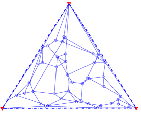
Refer to caption
Refer to caption
Figure 4: Effect of communication noise and link failures: (a) An N=50𝑁50N=50 node network and the respective triangulation sets. (d) DLRE (with a decreasing weight sequence, α=4t+1𝛼4𝑡1\alpha=\frac{4}{t+1}) implemented on the network in (a), where the iterations are shown for two arbitrarily chosen sensors.

DILOC with Noisy Distance measurements: We now consider noise on the distance measurements. We assume that we have a reasonable estimate of the required distances such that it translates into a small perturbation of the system matrices, 𝐁^(t)^𝐁𝑡\mathbf{\widehat{B}}(t) and 𝐏^(t)^𝐏𝑡\mathbf{\widehat{P}}(t). The matrices 𝐒~𝐏,𝐒~𝐁subscript~𝐒𝐏subscript~𝐒𝐁\mathbf{\widetilde{S}}_{\mathbf{P}},\mathbf{\widetilde{S}}_{\mathbf{B}} are zero-mean Gaussian i.i.d. perturbations with variance 0.10.10.1 (small signal perturbation, note that the non-zero elements of both the matrices, 𝐁𝐁\mathbf{B} and 𝐏𝐏\mathbf{P} lie in the range of 00 and 111). For a network of N=50𝑁50N=50 nodes in Fig. 5, we implement DLRE, with a decreasing weight sequence, α=1t0.55𝛼1superscript𝑡0.55\alpha=\frac{1}{t^{0}.55}, in Fig. 5. Finally, Fig. 6 shows a network of N=50𝑁50N=50 nodes, where DLRE, with a decreasing weight sequence, α=1t0.55𝛼1superscript𝑡0.55\alpha=\frac{1}{t^{0}.55}, with all of the above random scenarios is implemented in Fig. 6.
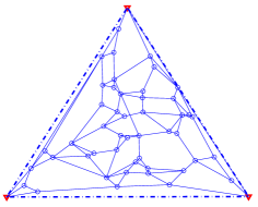
Refer to caption
Refer to caption
Figure 5: Effect of noisy distance measurements: (a) An N=50𝑁50N=50 node network and the respective triangulation sets. (d) DLRE (with a decreasing weight sequence, α=1t0.55𝛼1superscript𝑡0.55\alpha=\frac{1}{t^{0}.55}) implemented on the network in (a), where the iterations are shown for two arbitrarily chosen sensors.
Refer to caption
Refer to caption
Figure 6: Random environments (Noisy distances, communication noise, link failures): (a) An N=50𝑁50N=50 node network and the respective triangulation sets. (d) DLRE (with a decreasing weight sequence, α=1t0.55𝛼1superscript𝑡0.55\alpha=\frac{1}{t^{0}.55}) implemented on the network in (a), where the iterations are shown for two arbitrarily chosen sensors.

VIII Conclusions

The paper studies a distributed iterative sensor localization algorithm in  mlimit-from𝑚m-dimensional Euclidean space, m(m1)superscript𝑚𝑚1\mathbb{R}^{m}~{}(m\geq 1), that finds the location coordinates of the sensors in a sensor network with only local communication. The algorithm uses the minimal number, m+1𝑚1m+1, of anchors (sensors with known location) to localize an arbitrary number, M𝑀M, of sensors that lie in the convex hull of these m+1𝑚1m+1 anchors. In the deterministic case, i.e., when no noise affects the inter-sensor communication, the inter-sensor distances are known with no errors, and the communication links do not fail, we show that our distributed algorithms, DILOC and DILOC-REL, lead to convergence to the exact sensor locations. For the random environment scenario, where inter-sensor communication links may fail randomly, transmitted data is distorted by noise, and inter-sensor distance information is imprecise, we show that our modified algorithm, DLRE, leads to almost sure convergence of the iterative location estimates, and in this case we explicitly characterize the resulting error between the exact sensor locations and the converged estimates. Numerical simulations illustrate the behavior of the algorithms under different field conditions.

Appendix A Convex Hull Inclusion test

We now give an algorithm that tests if a given sensor, lm𝑙superscript𝑚l\in\mathbb{R}^{m}, lies in the convex hull of m+1𝑚1m+1 nodes in a set, κ𝜅\kappa, using only the mutual distance information among these m+2𝑚2m+2 nodes (κ{l}𝜅𝑙\kappa\cup\{l\}). Let κ𝜅\kappa denote the set of m+1𝑚1m+1 nodes and let 𝒞(κ)𝒞𝜅\mathcal{C}(\kappa) denote the convex hull formed by the nodes in κ𝜅\kappa. Clearly, if l𝒞(κ)𝑙𝒞𝜅l\in\mathcal{C}(\kappa), then the convex hull formed by the nodes in κ𝜅\kappa is the same as the convex hull formed by the nodes in κ{l}𝜅𝑙\kappa\cup\{l\}, i.e.,

𝒞(κ)=𝒞(κ{l}),if l𝒞(κ).formulae-sequence𝒞𝜅𝒞𝜅𝑙if 𝑙𝒞𝜅\mathcal{C}(\kappa)=\mathcal{C}(\kappa\cup\{l\}),\qquad\mbox{if }l\in\mathcal{C}(\kappa). (114)

With the above equation, we can see that, if l𝒞(κ)𝑙𝒞𝜅l\in\mathcal{C}(\kappa), then the generalized volumes of the two convex sets, 𝒞(κ)𝒞𝜅\mathcal{C}(\kappa) and 𝒞(κ{l})𝒞𝜅𝑙\mathcal{C}(\kappa\cup\{l\}), should be equal. Let Aκsubscript𝐴𝜅A_{\kappa} denote the generalized volume of 𝒞(κ)𝒞𝜅\mathcal{C}(\kappa) and let Aκ{l}subscript𝐴𝜅𝑙A_{\kappa\cup\{l\}} denote the generalized volume of 𝒞(κ{l})𝒞𝜅𝑙\mathcal{C}(\kappa\cup\{l\}), we have

Aκsubscript𝐴𝜅\displaystyle A_{\kappa} =\displaystyle= Aκ{l},subscript𝐴𝜅𝑙\displaystyle A_{\kappa\cup\{l\}}, (115)
=\displaystyle= kκAκ{l}{k},if l𝒞(κ).subscript𝑘𝜅subscript𝐴𝜅𝑙𝑘if 𝑙𝒞𝜅\displaystyle\sum_{k\in\kappa}A_{\kappa\cup\{l\}\setminus\{k\}},\qquad\mbox{if }l\in\mathcal{C}(\kappa).

Hence, the test becomes

l𝒞(κ),ifkκAκ{l}{k}=Aκ,formulae-sequence𝑙𝒞𝜅ifsubscript𝑘𝜅subscript𝐴𝜅𝑙𝑘subscript𝐴𝜅\displaystyle l\in\mathcal{C}(\kappa),\qquad\mbox{if}\,\,\sum_{k\in\kappa}A_{\kappa\cup\{l\}\setminus\{k\}}=A_{\kappa}, (116)
l𝒞(κ),ifkκAκ{l}{k}>Aκ.formulae-sequence𝑙𝒞𝜅ifsubscript𝑘𝜅subscript𝐴𝜅𝑙𝑘subscript𝐴𝜅\displaystyle l\notin\mathcal{C}(\kappa),\qquad\mbox{if}\,\,\sum_{k\in\kappa}A_{\kappa\cup\{l\}\setminus\{k\}}>A_{\kappa}. (117)

This is also shown in Figure 7. The above inclusion test is based entirely on the generalized volumes, which can be calculated using only the distance information in the Cayley-Menger determinants.
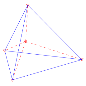
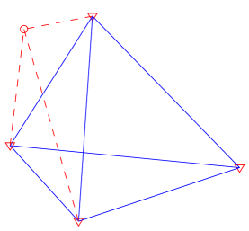
Refer to caption
Refer to caption
Figure 7: Convex Hull Inclusion Test (m=3): The sensor l𝑙l is shown by a ‘\circ’, whereas, the anchors in κ𝜅\kappa are shown by ‘\nabla’. (a) l𝒞(κ)Aκ=Aκ{l}𝑙𝒞𝜅subscript𝐴𝜅subscript𝐴𝜅𝑙l\in\mathcal{C}(\kappa)\Rightarrow A_{\kappa}=A_{\kappa\cup\{l\}}, (b) l𝒞(κ)Aκ<Aκ{l}𝑙𝒞𝜅subscript𝐴𝜅subscript𝐴𝜅𝑙l\notin\mathcal{C}(\kappa)\Rightarrow A_{\kappa}<A_{\kappa\cup\{l\}}.

Appendix B Cayley-Menger Determinant

Let κ𝜅\kappa be a set of m+1𝑚1m+1 points (sensors) in msuperscript𝑚\mathbb{R}^{m}, and dljsubscript𝑑𝑙𝑗d_{lj} be the inter-sensor distance between l𝑙l and j𝑗j. The generalized volume, Aκsubscript𝐴𝜅A_{\kappa}, of the convex hull of the points in κ𝜅\kappa can be computed by the Cayley-Menger determinant, see, e.g., [33]. The Cayley-Menger determinant is the determinant of an m+2×m+2𝑚2𝑚2m+2\times m+2 (symmetric) matrix that relates to the generalized volume, Aκsubscript𝐴𝜅A_{\kappa}, of the convex hull,  𝒞(κ)𝒞𝜅\mathcal{C}(\kappa), of the m+1𝑚1m+1 points in msuperscript𝑚\mathbb{R}^{m} through an integer sequence, sm+1subscript𝑠𝑚1s_{m+1}. The Cayley-Menger determinant is given by

sm+1Aκ2=|0111110d122d132d1,m+121d2120d232d242d2,m+121d312d3220d342d422d4320dm1,m+12dm,m+121dm+1,12dm+1,12dm+1,m12dm+1,m20|,subscript𝑠𝑚1superscriptsubscript𝐴𝜅20111missing-subexpression110superscriptsubscript𝑑122superscriptsubscript𝑑132missing-subexpressionsuperscriptsubscript𝑑1𝑚121superscriptsubscript𝑑2120superscriptsubscript𝑑232superscriptsubscript𝑑242superscriptsubscript𝑑2𝑚121superscriptsubscript𝑑312superscriptsubscript𝑑3220superscriptsubscript𝑑342missing-subexpressionmissing-subexpressionsuperscriptsubscript𝑑422superscriptsubscript𝑑4320superscriptsubscript𝑑𝑚1𝑚12superscriptsubscript𝑑𝑚𝑚121superscriptsubscript𝑑𝑚112superscriptsubscript𝑑𝑚112superscriptsubscript𝑑𝑚1𝑚12superscriptsubscript𝑑𝑚1𝑚20s_{m+1}A_{\kappa}^{2}=\left|\begin{array}[]{ccccccc}0&1&1&1&&\ldots&1\\ 1&0&d_{12}^{2}&d_{13}^{2}&&\ldots&d_{1,m+1}^{2}\\ 1&d_{21}^{2}&0&d_{23}^{2}&d_{24}^{2}&\ldots&d_{2,m+1}^{2}\\ 1&d_{31}^{2}&d_{32}^{2}&0&d_{34}^{2}&\ddots&\vdots\\ &&d_{42}^{2}&d_{43}^{2}&0&\ddots&d_{m-1,m+1}^{2}\\ \vdots&\vdots&\vdots&\ddots&\ddots&\ddots&d_{m,m+1}^{2}\\ 1&d_{m+1,1}^{2}&d_{m+1,1}^{2}&\ldots&d_{m+1,m-1}^{2}&d_{m+1,m}^{2}&0\end{array}\right|, (118)

where

sm=(1)m+12m(m!)2,m={0,1,2,},formulae-sequencesubscript𝑠𝑚superscript1𝑚1superscript2𝑚superscript𝑚2𝑚012s_{m}={(-1)^{m+1}}{2^{m}(m!)^{2}},\qquad\qquad m=\{0,1,2,\ldots\}, (119)

and its first few terms are 1,2,16,288,9216,460800,.12162889216460800-1,2,-16,288,-9216,460800,\ldots.

Appendix C Important Results

Lemma 5

If the matrix, 𝐏𝐏\mathbf{P}, corresponds to the transition probability matrix associated to the transient states of an absorbing Markov chain, then

limt𝐏t+1subscript𝑡superscript𝐏𝑡1\displaystyle\lim_{t\rightarrow\infty}\mathbf{\mathbf{P}}^{t+1} =\displaystyle= 𝟎.0\displaystyle\mathbf{0}. (120)
Proof.

For such a matrix, 𝐏𝐏\mathbf{P}, we have

ρ(𝐏)<1,𝜌𝐏1\rho(\mathbf{P})<1, (121)

from Lemma 8.3.20 and Theorem 8.3.21 in [34], where ρ()𝜌\rho(\cdot) denotes the spectral norm of a matrix and (120) follows from (121). ∎

Lemma 6

If the matrix, 𝐏𝐏\mathbf{P}, corresponds to the transition probability matrix associated to the transient states of an absorbing Markov chain, then

limtk=0t+1𝐏ksubscript𝑡superscriptsubscript𝑘0𝑡1superscript𝐏𝑘\displaystyle\lim_{t\rightarrow\infty}\sum_{k=0}^{t+1}\mathbf{\mathbf{P}}^{k} =\displaystyle= (𝐈𝐏)1.superscript𝐈𝐏1\displaystyle\left(\mathbf{\mathbf{I}-\mathbf{P}}\right)^{-1}. (122)
Proof.

The proof follows from Lemma 5 and Lemma 6.2.1 in [34]. ∎

References

  • [1] Usman A. Khan and José M. F. Moura, “Distributing the Kalman filters for large-scale systems,” IEEE Transactions on Signal Processing, Aug. 2007, accepted for publicaiton, DOI: 10.1109/TSP.2008.927480.
  • [2] G. Springer, Introduction to Riemann surfaces, Addison-Wesley, Reading, MA, 1957.
  • [3] J. G. Hocking and G. S. Young, Topology, Addison-Wesley, Reading, MA, 1961.
  • [4] R. L. Moses, D. Krishnamurthy, and R. Patterson, “A self-localization method for wireless sensor networks,” EURASIP Journal on Applied Signal Processing, , no. 4, pp. 348–358, Mar. 2003.
  • [5] N. Patwari, A. O. Hero III, M. Perkins, N. Correal, and R. J. O Dea, “Relative location estimation in wireless sensor networks,” IEEE Trans. on Signal Processing, vol. 51, no. 8, pp. 2137–2148, Aug. 2003.
  • [6] Y. Shang, W. Ruml, Y. Zhang, and M. Fromherz, “Localization from mere connectivity,” in 4th ACM international symposium on mobile ad-hoc networking and computing, Annapolis, MD, Jun. 2003, pp. 201–212.
  • [7] Y. Shang and W. Ruml, “Improved MDS-based localization,” in IEEE Infocom, Hong Kong, Mar. 2004, pp. 2640–2651.
  • [8] F. Thomas and L. Ros, “Revisiting trilateration for robot localization,” IEEE Transactions on Robotics, vol. 21, no. 1, pp. 93–101, Feb. 2005.
  • [9] M. Cao, B. D. O. Anderson, and A. S. Morse, “Localization with imprecise distance information in sensor networks,” Sevilla, Spain, Dec. 2005, pp. 2829–2834.
  • [10] S. T. Roweis and L. K. Saul, “Nonlinear dimensionality reduction by local linear embedding,” Science, vol. 290, pp. 2323–2326, Dec. 2000.
  • [11] N. Patwari and A. O. Hero III, “Manifold learning algorithms for localization in wireless sensor networks,” in IEEE International Conference on Sig. Proc., Montreal, Canada, Mar. 2004, vol. 3, pp. 857–860.
  • [12] D. Niculescu and B. Nath, “Ad-hoc positioning system,” in IEEE Globecom, Apr. 2001, pp. 2926–2931.
  • [13] A. Savvides, C. C. Han, and M. B. Srivastava, “Dynamic fine-grained localization in ad-hoc networks of sensors,” in IEEE Mobicom, Rome, Italy, Jul. 2001, pp. 166–179.
  • [14] A. Savvides, H. Park, and M. B. Srivastava, “The bits and flops of the N-hop multilateration primitive for node localization problems,” in Intl. Workshop on Sensor Networks and Applications, Atlanta, GA, Sep. 2002, pp. 112–121.
  • [15] R. Nagpal, H. Shrobe, and J. Bachrach, “Organizing a global coordinate system from local information on an ad-hoc sensor network,” in 2nd Intl. Workshop on Information Processing in Sensor Networks, Palo Alto, CA, Apr. 2003, pp. 333–348.
  • [16] J. J. Caffery, Wireless location in CDMA cellular radio systems, Kluwer Academic Publishers, Norwell, MA, 1999.
  • [17] J. A. Costa, N. Patwari, and III A. O. Hero, “Distributed weighted-multidimensional scaling for node localization in sensor networks,” ACM Transactions on Sensor Networks, vol. 2, no. 1, pp. 39–64, 2006.
  • [18] J. Albowicz, A. Chen, and L. Zhang, “Recursive position estimation in sensor networks,” in IEEE Int. Conf. on Network Protocols, Riverside, CA, Nov. 2001, pp. 35–41.
  • [19] C. Savarese, J. M. Rabaey, and J. Beutel, “Locationing in distributed ad-hoc wireless sensor networks,” in IEEE International Conference on Sig. Proc., Salt Lake City, UA, May 2001, pp. 2037–2040.
  • [20] S. Čapkun, M. Hamdi, , and J. P. Hubaux, “GPS-free positioning in mobile ad-hoc networks,” in 34th IEEE Hawaii Int. Conf. on System Sciences, Wailea Maui, HI, Jan. 2001.
  • [21] A. T. Ihler, J. W. Fisher III, R. L. Moses, and A. S. Willsky, “Nonparametric belief propagation for self-calibration in sensor networks,” in IEEE International Conference on Sig. Proc., Montreal, Canada, May 2004.
  • [22] L. Hu and D. Evans, “Localization for mobile sensor networks,” in IEEE Mobicom, Philadelphia, PA, Sep. 2004, pp. 45–57.
  • [23] M. Coates, “Distributed particle filters for sensor networks,” in IEEE Information Processing in Sensor Networks, Berkeley, CA, Apr. 2004, pp. 99–107.
  • [24] S. Thrun, “Probabilistic robotics,” Communications of the ACM, vol. 45, no. 3, pp. 52–57, Mar. 2002.
  • [25] J. C. Gower, “Euclidean distance geometry,” Mathematical Scientist, vol. 7, pp. 1–14, 1982.
  • [26] J. C. Gower, “Propoerties of Euclidean and non-Euclidean distance matrices,” Linear Algebra and its Applications, vol. 67, pp. 81–97, Jun. 1985.
  • [27] P. Hall, Introduction to the theory of coverage processes, John Wiley and Sons Inc., Chichester, UK, 1988.
  • [28] Y. Sung, L. Tong, and A. Swami, “Asymptotic locally optimal detector for large-scale sensor networks under the poisson regime,” IEEE Transactions on Signal Processing, vol. 53, no. 6, pp. 2005–2017, Jun. 2005.
  • [29] C. M. Grinstead and J. L. Snell, Introduction to probability, American Mathematical Society, 1997.
  • [30] S. Kar and J. M. F. Moura, “Distributed consensus algorithms in sensor networks: Link failures and channel noise,” November 2007, Manuscript submitted to the IEEE Transactions on Signal Processing, http://arxiv.org/abs/0711.3915.
  • [31] S. Kar and J. M. F. Moura, “Distributed consensus algorithms in sensor networks: Quantized data,” December 2007, Manuscript submitted to the IEEE Transactions on Signal Processing, http://aps.arxiv.org/abs/0712.1609.
  • [32] M.B. Nevel’son and R.Z. Has’minskii, Stochastic approximation and recursive estimation, American Mathematical Society, Providence, Rhode Island, 1973.
  • [33] M. J. Sippl and H. A. Scheraga, “Cayley–Menger coordinates,” Proceedings of the National Academy of Sciences of U.S.A., vol. 83, no. 8, pp. 2283–2287, Apr. 1986.
  • [34] A. Berman and R. J. Plemmons, Nonnegative matrices in the mathematical sciences, Academic Press, INC., New York, NY, 1970.