Abstract

Quantum ergodicity asserts that almost all infinite sequences of eigenstates of a quantized ergodic system are equidistributed in the phase space. On the other hand, there are might exist exceptional sequences which converge to different (non-Liouville) classical invariant measures $\mu$. By the remarkable result of N. Anantharaman and S. Nonnenmacher math-ph/0610019, arXiv:0704.1564 (with H. Koch), for Anosov geodesic flows the metric entropy of any semiclassical measure $\mu$ must be bounded from below. The result seems to be optimal for uniformly expanding systems, but not in general case, where it might become even trivial if the curvature of the Riemannian manifold is strongly non-uniform. It has been conjectured by the same authors, that in fact, a stronger bound (valid in general case) should hold.

In the present work we consider such entropic bounds using the model of quantized one-dimensional maps. For a certain class of non-uniformly expanding maps we prove Anantharaman-Nonnenmacher conjecture. Furthermore, for these maps we are able to construct some explicit sequences of eigenstates which saturate the bound. This demonstrates that the conjectured bound is actually optimal in that case.

1 Introduction

The theory of quantum chaos concerns with the quantum systems whose classical limit is chaotic. It is assumed in general, that chaotic dynamics induce certain characteristic patterns. For instance, the Random Matrix conjecture predicts that statistical distribution of high-lying eigenvalues in a chaotic system is the same as in certain ensembles of random matrices and depends only on symmetries of the system [1]. In the same spirit, it is believed that eigenstates of chaotic systems are delocalized over the whole available part of the phase space [2], [3] which is totally different from the case of integrable dynamics, where eigenstates are known to concentrate near KAM tori [4]. The rigorous implementation of that idea is known as Quantum Ergodicity Theorem. It was first proven by A. I. Schnirelman for Laplacians on surfaces of negative curvature [5] and later generalized [6], [7] and extended to other systems e.g., ergodic billiards [8, 9], quantized maps [10] and general Hamiltonians [11].

Very generally, the Quantum Ergodicity Theorem states that for a classically ergodic system “almost all” eigenstates in the semiclassical regime become uniformly distributed over the phase space. To give the precise meaning of such a statement it is convenient to use the notion of measure. For a Hamiltonian system a sequence of the eigenstates $\{\psi_{\Bbbk},\,\,\Bbbk=1,\dots\infty\}$ generates the corresponding sequence of the measures $\{d\mu_{\Bbbk}=W_{\Bbbk}(x,\xi)\,dxd\xi,\,\,\Bbbk=1,\dots\infty\}$ on the classical phase space, where the density $W_{\Bbbk}(x,\xi)$ can be interpreted as the “distribution” of $\psi_{\Bbbk}$ over the phase space. Although the exact form of $W_{\Bbbk}$ depends on the quantization procedure (e.g., Weyl, Anti-Wick quantization etc.), the limiting semiclassical measure:

$$\lim_{\Bbbk\to\infty}\mu_{\Bbbk}=\mu,$$ (1)

is invariant under the corresponding classical flow and does not depend on the choice of the quantization. The Quantum Ergodicity theorem asserts that for “almost all” sequences of the eigenstates the limiting measure $\mu$ is actually the Liouville measure.

Since the Quantum Ergodicity theorem does not exclude possibility that exceptional sequences of eigenstates produce non-Liouville classically invariant measures, it makes sense to ask whether such measures might actually appear. In the context of Anosov geodesic flows on surfaces of negative curvature it was conjectured [12] that a typical system posses “Quantum Unique Ergodicity” property, meaning that all sequences of eigenstates converge to the Liouville measure. However, there have been only a limited number of rigorous results supporting this conjecture. So far, the most important one was obtained by E. Lindenstrauss. In [13] he proved that all Hecke eigenstates of the Laplacian on compact arithmetic surfaces are equidistributed. If (as widely believed) all the Laplacian eigenstates are non-degenerate, this result would amount to the proof of Quantum Unique Ergodicity for the arithmetic case. On the other hand, it is known that exceptional sequences actually do appear in some quantum systems. For quantum “cat maps” such sequences were identified in [14] [15]. The limiting measure there could be, for instance, composed of two ergodic components:

$$\mu=a\mu_{{\scriptscriptstyle\mathrm{L}}}+(1-a)\mu_{{\scriptscriptstyle\mathrm{D}}},\qquad 1\geq a\geq 1/2,$$ (2)

where the first part $\mu_{{\scriptscriptstyle\mathrm{L}}}$ is the Liouville measure equidistributed over the whole phase space and the second part $\mu_{{\scriptscriptstyle\mathrm{D}}}$ is the Dirac peak concentrated on a single unstable periodic orbit. Similar sequences of eigenstates have been also constructed for the “Walsh quantization“ of the baker’s map [16]. For quantized hyperbolic automorphisms of higher-dimensional tori there exists a different type of semiclassical measures which are Lebesgue measures on some invariant co-isotropic subspaces of the torus [17].

As we know that non-Liouville semiclassical measures do appear (at least) in some systems, it would be of great interest to understand which kind of them might exist in a general case. Quite recently, it has been proven by N. Anantharaman and S. Nonnenmacher [18], [19], [20] (with H. Koch) that for the Laplacian on a compact Riemannian manifold with Anosov geodesic flow the metric (Kolmogorov-Sinai) entropy $H_{{\scriptscriptstyle\mathrm{KS}}}(\mu)$ of any semiclassical measure $\mu$ must satisfy certain bound. Particularly, in the two-dimensional case the following result holds [20]:

$$H_{{\scriptscriptstyle\mathrm{KS}}}(\mu)\geq\int|\log J^{u}(x)|d\mu-\frac{1}{2}\lambda_{\max},$$ (3)

where $J^{u}(x)$ is the unstable Jacobian of the flow at the point $x$ and $\lambda_{\max}$ is the maximum expansion rate of the flow. If the maximum expansion rate is close to its average value, this remarkable bound gives a valuable information on $\mu$ itself. In particular, for surfaces with a constant negative curvature this remarkable bound implies that maximum “half” of the measure might concentrate on periodic orbits. On the other hand, if the expansion rate varies a lot, the above bound does not give any information, as the right hand side of (3) becomes negative. Thus, it is natural to expect that (3) is not an optimal result, and a stronger bound might exist in a general case. Such a bound has been conjectured in [18, 16]. It states that for chaotic systems a semiclassical measure must satisfy:

$$H_{{\scriptscriptstyle\mathrm{KS}}}(\mu)\geq\frac{1}{2}\int|\log J^{u}(x)|d\mu.$$ (4)

Assuming that the conjecture is true, it provides a restriction on the class of possible semiclassical measures in general case. In particular, for semiclassical measures of the type (2) the bound (4) would imply that Liouville part should be always present and its proportion satisfy $a\geq\frac{\lambda_{\scriptscriptstyle\mathrm{D}}}{\lambda_{\mathrm{av}}+\lambda_{\scriptscriptstyle\mathrm{D}}}$, where $\lambda_{\mathrm{av}}$ is the average Laypunov exponent (with respect to the Liouville measure) and $\lambda_{\scriptscriptstyle\mathrm{D}}$ is the Laypunov exponent for the periodic orbit where $\mu_{{\scriptscriptstyle\mathrm{D}}}$ is localized.

2 Model and statement of the main results

The central purpose of this paper is to provide support for the conjectured bound (4) using the model of quantized one-dimensional piecewise linear maps. A procedure for quantization of one-dimensional linear maps was originally introduced in [21] in order to generate families of quantum graphs with some special properties. Being much simpler on the technical level, these models still exhibit characteristic properties of typical quantum chaotic Hamiltonian systems. Most importantly, it turns out that the quantum evolution here follows the classical evolution till the (Ehrenfest) time which grows logarithmically with the dimension of the Hilbert space. Note also that, as will be shown in the body of the paper, the construction is closely related to the Walsh quantized baker’s maps in [16].

In the present work we will consider Lebesgue measure preserving maps $T:[0,1]\to[0,1]=:I$ consisting of several linear branches. More specifically, let $\{I_{j},\,\,j=1,\dots l\}$ be a partition of the unite interval $I=\cup^{l}_{j=1}I_{j}$ into $l$ subintervals. At each subinterval $I_{j}$, $T$ is then defined as a simple linear map $T:I_{j}\to I$:

$$T(x)=x\Lambda_{j}+b_{j},\qquad\mbox{ for }x\in I_{j},\,\,\,j=1,\dots l.$$ (5)

Conditions 1.

We consider maps $T$ of the form (5) satisfying the following conditions:

• $\sum^{l}_{j=1}\Lambda^{-1}_{j}=1$ and $\Lambda_{i}$, $i=1,\cdots l$ are integers larger then one.

• Each subinterval $I_{j}$ is mapped by $T$ upon the whole unite interval $I$. Correspondingly, the Lebesgue measure of each $I_{j}$ equals to $\Lambda^{-1}_{j}$ and $b_{1}=0$, $b_{i}=-\Lambda_{i}(\sum_{k<i}\Lambda_{k}^{-1})$ for $1<i\leq l$.

Remark 1.

The first condition above is essential. It implies that the map is Lebesgue measure preserving, chaotic and the set of endpoints of partitions $\mathcal{M}_{\Bbbk}$ is forward invariant under the action of $T$ (see below). The second condition is imposed solely for the sake of simplicity of exposition. It implies that $i$’s branch of $T$ “starts” from a point $x_{i}$, where $T(x_{i})=0$ and “ends” at the point $x_{i+1}$, where $T(x_{i+1})=1$. In principle, most of the results of the paper can be extended to a more general class of expanding piecewise linear maps considered in [21].

We will now briefly describe the procedure introduced by P. Pakoński et al [21] for quantization of such maps. Let $\mathcal{M}=\{E_{i},\,\,i=0,\dots N-1\}$ be the partition of $I$ into $N$ intervals $E_{i}=[i/N,(i+1)/N]$, $i=0,\cdots N-1$ of equal lengths. For the interval $E_{i}$ we will denote by $\beta_{+}(E_{i})$ ($\beta_{-}(E_{i})$) right (resp. left) endpoint of $E_{i}$ and by $\beta(\mathcal{M})=\cup_{i=1}^{N}\beta_{\pm}(E_{i})$ the set of all endpoints of the partition $\mathcal{M}$. Obviously both $\mathcal{M}$ and $\beta(\mathcal{M})$ are uniquely determined by the size $N$ of the partition. In what follows we will consider an increasingly refined sequence of the above partitions $\mathcal{M}_{\Bbbk}$ with the sizes $N_{\Bbbk}$, $\Bbbk=1,\dots\infty$.

Conditions 2.

Given a map $T$ satisfying Conditions 1 we impose the following conditions on the sequence of $\mathcal{M}_{\Bbbk}$:

• Each partition $\mathcal{M}_{\Bbbk}$ is a refinement of the previous one. That means for each $\Bbbk\geq 1$, $N_{\Bbbk+1}/N_{\Bbbk}$ is an integer number greater then one.

• The set of the endpoints of the initial partition $\mathcal{M}_{1}$ must include all singular points of $T$ i.e., $\beta(\mathcal{M}_{1})\supseteq\beta(I_{i})$ for all $i=1,\dots l$.

For a map $T$ satisfying Conditions 1 and a sequence of partitions $\mathcal{M}_{\Bbbk}$, $\Bbbk=1,\dots\infty$ satisfying Conditions 2 consider the sequence of the corresponding transfer (Frobenius-Perron) operators given by $N_{\Bbbk}\times N_{\Bbbk}$ doubly stochastic matrices $B_{\Bbbk}$, whose elements read as:

$$B_{\Bbbk}(i,j)=\frac{|E_{i}\cap T^{-1}E_{j}|}{|E_{i}|}=\left\{\begin{array}[]{lc}\Lambda_{i}^{-1}&\mbox{ if }E_{i}\cap T^{-1}E_{j}\neq\emptyset\\ 0&\mbox{ otherwise. }\end{array}\right.$$ (6)

We will call a piecewise linear map $T$ quantizable if there exists a sequence of partitions $\mathcal{M}_{\Bbbk}$, $\Bbbk=1,\dots\infty$ such that for each matrix $B_{\Bbbk}$ one can find a unitary matrix $U_{\Bbbk}$ of the same dimension satisfying

$$B_{\Bbbk}(j,i)=|U_{\Bbbk}(i,j)|^{2}.$$ (7)

for each matrix element $(j,i)$; $j,i\in\{1,\dots N_{\Bbbk}\}$. For quantizable maps the matrices $U_{\Bbbk}$ are regarded as “quantizations” of $B_{\Bbbk}$ and play the role of quantum evolution operators acting on $N_{\Bbbk}$-dimensional Hilbert space $\mathcal{H}_{\Bbbk}\simeq\mathbbm{C}^{N_{\Bbbk}}$. As an example, consider the following linear map (see fig. 1a):

$$T(x)=2x\mod 1,\qquad x\in[0,1].$$ (8)

Figure 1: Linear maps with uniform (left) and non-uniform slopes (right) which allow “tensorial” quantization.

Here for the sequence of partitions $\mathcal{M}_{\Bbbk}$ of the unite interval into $N_{\Bbbk}=2^{\Bbbk}$ equal pieces, the matrix elements $B_{\Bbbk}(i,j)$ of the classical transfer operators take the values $1/2$ if $j=2i$, $j=2i-1$, $j+N_{\Bbbk}=2i$, $j+N_{\Bbbk}=2i-1$ and $0$ otherwise:

$$B_{2}=\frac{1}{2}\left(\begin{array}[]{cc}1&1\\ 1&1\\ \end{array}\right),\qquad B_{4}=\frac{1}{2}\left(\begin{array}[]{cccc}1&1&0&0\\ 0&0&1&1\\ 1&1&0&0\\ 0&0&1&1\\ \end{array}\right),\qquad\cdots$$

Note that the structure of $B_{\Bbbk}$, actually, resembles the structure of the map $T$ (rotated clockwise by $\pi/2$). It is easy to see that the map (8) is quantizable. By a permutation of rows $B_{\Bbbk}$ can be brought into the block diagonal form such that every block is $2\times 2$ matrix $B_{2}$ whose all elements are $1/2$. Thus the question of the quantization of $T$ reduces to finding of a unitary $2\times 2$ matrix $\mathbf{U}$ satisfying $|\mathbf{U}(l,m)|^{2}=1/2$ for all its elements. The appropriate choice is given, for instance, by the discrete Fourier transform: $\mathbf{U}(l,m)=\frac{1}{\sqrt{2}}\exp{(\pi ilm)}$. This example can be straightforwardly generalized to all other maps with a uniform slope. The question of the quantizability of general piecewise linear maps will be discussed in the body of the paper.

Note that the above quantization of one-dimensional piecewise linear maps is just a formal procedure for generation of unitary matrices $U_{\Bbbk}$. To turn it to a “meaningful” quantization one needs, in addition, to make a connection between classical observables on the unite interval and the corresponding quantum observables on the Hilbert space $\mathcal{H}_{\Bbbk}$. Such a quantization procedure has been introduced in [22]. With a classical observable $f\in L^{2}[0,1]$ one associates the sequence of the quantum observables $\mathbf{Op}_{\Bbbk}(f)$, defined by the diagonal matrices of the dimension $N_{\Bbbk}$ whose components $\mathbf{Op}_{\Bbbk}(f)_{j,j}$ equal to the average value of $f$ at $j$’s element of the partition $\mathcal{M}_{\Bbbk}$. The key observation making the above quantization interesting is the existence of the semiclassical correspondence (Egorov property) between evolutions of classical and quantum observables. Precisely, for a Lipschitz continues observable $f(x)$ one has [22]:

$$||U^{*}_{\Bbbk}\mathbf{Op}_{\Bbbk}(f)U_{\Bbbk}-\mathbf{Op}_{\Bbbk}(f\circ T)||=O\left(\frac{1}{N_{\Bbbk}}\right).$$ (10)

Note that, the size of the partition $N^{-1}_{\Bbbk}$ plays here the role of the Planck constant and the semiclassical limit corresponds to $\Bbbk\to\infty$.

Equipped with the above quantization procedure we can define now the sequence of the semiclassical measures associated with the eigenstates of $U_{\Bbbk}$. For $\psi_{\Bbbk}\in\mathcal{H}_{\Bbbk}$, $U_{\Bbbk}\psi_{\Bbbk}=e^{i\theta_{\Bbbk}}\psi_{\Bbbk}$, $\Bbbk=1,\cdots\infty$ we define $\mu_{\Bbbk}$ through the relationship:

$$\int_{I}f(x)\,d\mu_{\Bbbk}(x)=\langle\psi_{\Bbbk}\mathbf{Op}_{\Bbbk}(f)\psi_{\Bbbk}\rangle.$$ (11)

We will be concerned with the possible semiclassical limits of $\mu_{\Bbbk}$ as $\Bbbk\to\infty$ and call any such limiting measure $\mu$ as semiclassical measure. Speaking informally $\mu$ characterizes the possible sets of the localization on the interval $[0,1]$ of the eigenstates of quantized maps. (An alternative point of view (see [22]) is to look at such limits as “scars” on the sequence of quantum graphs defined by $U_{\Bbbk}$.) An immediate consequence of the Egorov property is that any semiclassical measure $\mu$ must be invariant under the map $T$. Indeed, since $\psi_{\Bbbk}$ is an eigenstate of $U_{\Bbbk}$:

$$\int_{I}f(x)\,d\mu_{\Bbbk}(x)=\langle\psi_{\Bbbk}\,U_{\Bbbk}^{*}\mathbf{Op}_{\Bbbk}(f)U_{\Bbbk}\psi_{\Bbbk}\rangle=\int_{I}f(T(x))\,d\mu_{\Bbbk}(x)+O\left(\frac{1}{N_{\Bbbk}}\right),$$ (12)

and the invariance of $\mu$ follows immediately after taking the limit $\Bbbk\to\infty$. As there exist many classical measures preserved by $T$, the invariance alone does not determine all possible outcomes for the semiclassical measures. Similarly to Hamiltonian systems, using Egorov property one can show by standard methods (see e.g., [25]) that almost any sequence of the eigenstates gives rise to the Lebesgue measure in the semiclassical limit (this was proved in [22] by somewhat a different method).

Theorem 1.

(Quantum Ergodicity [22, Thm. 2].) Let $T$ be a quantizable map (5) satisfying Condition 1 and let $U_{\Bbbk}$, $\Bbbk=1,\dots\infty$ be a sequence of its quantizations with eigenstates $\psi^{(i)}_{\Bbbk}$, $i=1,\dots N_{\Bbbk}$. Then for each $\Bbbk$ there exists subsequence of $\mathcal{N}_{\Bbbk}$ eigenstates: $\boldsymbol{\Psi}_{\Bbbk}:=\{\psi^{(i_{1})}_{\Bbbk},\dots\psi^{(i_{\mathcal{N}_{\Bbbk}})}_{\Bbbk}\}$ such that $\lim_{\Bbbk\to\infty}\mathcal{N}_{\Bbbk}/N_{\Bbbk}=1$ and for any sequence of eigenstates $\psi_{\Bbbk_{j}}\in\boldsymbol{\Psi}_{\Bbbk_{j}}$, $j=1,\dots\infty$ and a Lipschitz continues function $f$ one has:

$$\lim_{j\to\infty}\langle\psi_{\Bbbk_{j}}\mathbf{Op}_{\Bbbk_{j}}(f)\psi_{\Bbbk_{j}}\rangle=\int_{I}f(x)\,dx.$$ (13)

In the present paper we go beyond the Quantum Ergodicity and ask about the possible exceptional semiclassical measures. Our first result is the precise analog of the bound (3):

Theorem 2.

Let $T$ be a quantizable piecewise linear map (5) satisfying Condition 1. Let $U_{\Bbbk}$, $\Bbbk=1,\dots\infty$ be a sequence of its quantizations and let $\psi_{\Bbbk}$, $\Bbbk=1,\dots\infty$ be some subsequence of its eigenstates. Then the following bound holds for the metric entropy of the corresponding semiclassical measure $\mu$:

$$H_{{\scriptscriptstyle\mathrm{KS}}}(T,\mu)\geq\int_{I}\log\Lambda(x)\,d\mu(x)-\frac{1}{2}\log\Lambda_{\max}=\sum^{l}_{j=1}\mu(I_{j})\log\left(\Lambda_{j}\right)-\frac{1}{2}\log\Lambda_{\max},$$ (14)

where $\Lambda_{\max}:=\max_{1\leq j\leq l}\Lambda_{j}$ and $\mu(I_{j})$ are the measures of the intervals $I_{j}$.

As it is clear, that this bound is not optimal for the maps with non-uniform slopes, one would like to have a stronger result, analogous to the conjectured one (4). In the present we are able to prove such a bound for a particular subclass of piecewise linear maps (5). Namely, in the body of the paper we show that the maps $T_{p}$ whose slopes are given by the powers of the same integer number $p$ (see fig. 1b for an example of such a map), allow a special type of “tensorial” quantizations. For maps $T_{p}$ quantized in that way we prove the analog of Anantharaman-Nonnenmacher conjecture.

Theorem 3.

Let $T_{p}$ be a map of the form: $T_{p}(x)=\Lambda_{j}x\mod{1}$, $\Lambda_{j}=p^{n_{j}}$ for $x\in I_{j},j=1,2\dots l$ and let $U_{\Bbbk}$, $\Bbbk=1,\dots\infty$ be a sequence of “tensorial” quantization of $T_{p}$. Then for any sequence of eigenstates $\psi_{\Bbbk}$ of $U_{\Bbbk}$, $\Bbbk=1,\dots\infty$ the corresponding semiclassical measure $\mu$ satisfies:

$$H_{{\scriptscriptstyle\mathrm{KS}}}(T_{p},\mu)\geq\frac{1}{2}\sum^{l}_{j=1}\mu(I_{j})\log\left(\Lambda_{j}\right).$$ (15)

Furthermore, for these maps there exists an explicit construction of certain sequences of eigenstates of $U_{\Bbbk}$. Using these eigenstates we obtain a set of semiclassical measures which can be subsequently analyzed to test (15). It turns out that some of these semiclassical measures, in fact, saturate the bound implying that the result is sharp.

The paper is organized as follows. In Section 3 we deal with a general construction of unitary evolutions for piecewise-linear maps and prove “quantizability“ for a wide class of maps satisfying Conditions 1. Here we also introduce a special class of tensorial quantizations for the maps $T_{p}$ whose slopes are given by the powers of an integer $p$. In Section 4 we review the construction in [22] for quantization of observables and prove the Egorov property up to the Ehrenfest time. In Section 5 we connect metric entropy for the semiclassical measures with certain type of quantum observables. Based on the method of [19] we then prove Theorem 2 in Section 6 using the Entropic Uncertainty Principle. Section 7 is devoted to the proof of Theorem 15. Finally, in Section 8 we explicitly construct certain class of semiclassical measures for tensorial quantizations of maps $T_{p}$ and test the bound (15). The concluding remarks are presented in Section 9.

3 Quantization of one-dimensional piecewise linear maps

We will consider now in more details the quantizations of Lebesgue measure preserving piecewise linear maps $T$ of the form (5). Note that each map satisfying Condition 1 is uniquely determined by the ordered set of its slopes $\mathbf{\Lambda}=\{\Lambda_{1},\dots\Lambda_{l}\}$, so the notation $T=T_{\mathbf{\Lambda}}$ will be often used to define the corresponding map. Recall that a piecewise linear map $T_{\mathbf{\Lambda}}$ is ”quantizable” if there exists an infinite sequence of partitions $\mathcal{M}_{\Bbbk}$ of unite interval $I$ such that the corresponding evolution matrices $B_{\Bbbk}$ allow representation (7). In general, it is a non-trivial problem to determine whether a doubly stochastic matrix has such a representation in terms of a unitary matrix (see [21], [23] and references there). So, in principle, it is not clear in advance which of the maps $T_{\mathbf{\Lambda}}$ are actually “quantizable”. It is our purpose here to show that the class of quantizable piecewise linear maps is wide and contains many interesting maps.

3.1 General quantization

As has been already mentioned a map with a uniform slope is quantizable by means of the discrete Fourier transforms. Hence, a non-trivial question is about “quantizability” of the maps $T_{\mathbf{\Lambda}}$, $\mathbf{\Lambda}=\{\Lambda_{1},\dots\Lambda_{l}\}$ with at least two different $\Lambda_{i}$. Let $\Lambda_{i_{1}},\dots\Lambda_{i_{\ell}}$, $\ell>1$ be the maximal set of different slopes in $\mathbf{\Lambda}$, i.e., $\Lambda_{i_{n}}\neq\Lambda_{i_{m}}$ for $n\neq m$. Assuming that each slope $\Lambda_{i_{k}}$ has a multiplicity $m_{k}\geq 1$, the Lebesgue measure preservation condition

$$\sum_{k=1}^{\ell}\frac{m_{k}}{\Lambda_{i_{k}}}=1,$$ (16)

imposes certain restrictions on the values of $\Lambda_{i_{k}}$, $m_{k}$. In particular, it is clear that the set $\Lambda_{i_{k}},\,\,k=1,\dots\ell$ must have a greatest common divisor $p$ large then one. This means

$$\Lambda_{i_{k}}=p\bar{\Lambda}_{k}\qquad\bar{\Lambda}_{k}\in\mathbbm{N}\mbox{ for }k\in\{1,\dots\ell\}.$$

Assume now that all the numbers $\bar{\Lambda}_{i}$ are relatively prime. Then it follows immediately from (16) that $m_{k}$’s are of the form $m_{k}=\bar{m}_{k}\bar{\Lambda}_{k}$, $\bar{m}_{k}\in\mathbbm{N}$, $k\in\{1,\dots l\}$, where $\sum_{k=1}^{l}\bar{m}_{k}=p$. We are going now to show that the maps $T_{\mathbf{\Lambda}}$ whose slopes satisfy the above conditions are quantizable.

Theorem 4.

Let $T_{\mathbf{\Lambda}}$ be a map satisfying Condition 1 with the slopes $\Lambda_{i}=p\bar{\Lambda}_{i}$, $\bar{\Lambda}_{i+1}\geq\bar{\Lambda}_{i}$ of multiplicities $m_{i}$, $i\in\{1,\dots l\}$ such that $p\in\mathbbm{N}$ and $\bar{\Lambda}_{i}$’s are relatively prime integers, then $T_{\mathbf{\Lambda}}$ is “quantizable”.

Proof:

As the first step notice that $T_{\mathbf{\Lambda}}$ can be represented as the composition of the uniformly expanding map $\bar{T}_{p}$ and the ”block diagonal” map $T_{{\scriptscriptstyle\mathrm{BD}}}$, whose slopes are uniform at each block.

Lemma 1.

Let $T_{\mathbf{\Lambda}}$ be a map as defined above, then $T_{\mathbf{\Lambda}}=\bar{T}_{p}\circ T_{{\scriptscriptstyle\mathrm{BD}}}$, where $T_{p}(x)=xp\mod 1$ and

$$T_{{\scriptscriptstyle\mathrm{BD}}}(x)=\left(\Lambda_{i}x\mod 1\right)/p+b_{i},\qquad\mathrm{for}\,\,x\in[b_{i},b_{i+1}],\,\,\qquad b_{i}=\sum_{j<i}\frac{m_{j}}{\Lambda_{j}},$$

where $m_{i}$ is the multiplicity of $\bar{\Lambda}_{i}$.

Proof:

Straightforward calculation. $\Box$

The parameters entering into the definition of $T_{{\scriptscriptstyle\mathrm{BD}}}$ have the following simple meaning. The points $b_{i}$, $b_{i+1}$ mark the position of $i$’s block which is the square of the size $\frac{m_{j}}{\Lambda_{j}}$. Inside of each such block the map $T_{{\scriptscriptstyle\mathrm{BD}}}$ acts as a piecewise linear map with the uniform expansion rate $\bar{\Lambda}_{i}$.

Example. To illustrate the above lemma consider as an example the map with the slopes $6$ and $4$:

$$T(x)=\left\{\begin{array}[]{ll}6x\!\!\mod 1&\mbox{ if }x\in[0,1/2)\\ 4x\!\!\mod 1&\mbox{ if }x\in[1/2,1].\end{array}\right.$$ (17)

As shown in fig. 2, $T$ can be decomposed into the uniformly expanding map $\bar{T}_{2}=2x\!\!\mod 1$ and the ”block diagonal” map:

$$T_{{\scriptscriptstyle\mathrm{BD}}}(x)=\left\{\begin{array}[]{ll}(6x\!\!\mod 1)/2&\mbox{ if }x\in[0,1/2)\\ (4x\!\!\mod 1)/2+1/2&\mbox{ if }x\in[1/2,1].\end{array}\right.$$

Figure 2: A “generic” map (17) and its decomposition into the uniformly expanding and the ”block diagonal” parts.

Let us now define a set of partitions $\mathcal{M}_{\Bbbk}$ of $I$ by setting their seizes $N_{\Bbbk}$. Take $N_{0}=p\prod_{i=1}^{l}\bar{\Lambda}_{i}$, then $N_{\Bbbk}=(N_{0})^{\Bbbk}$ for $\Bbbk=\{0,\dots\infty\}$. It is clear that these partitions satisfy Conditions 2. For each partition $\mathcal{M}_{\Bbbk}$ denote by $\bar{B}_{\Bbbk}$, $B_{\Bbbk}^{{\scriptscriptstyle\mathrm{BD}}}$ the corresponding evolution operators for the map $\bar{T}_{p}$ and $T_{{\scriptscriptstyle\mathrm{BD}}}$ respectively. Note that both $\bar{B}_{\Bbbk}$ and $B_{\Bbbk}^{{\scriptscriptstyle\mathrm{BD}}}$ are quantizable i.e., one can find unitary matrices $\bar{U}_{\Bbbk}$, $U_{\Bbbk}^{{\scriptscriptstyle\mathrm{BD}}}$ satisfying (7). Indeed, this is completely obvious for $\bar{B}_{\Bbbk}$ as $\bar{T}_{p}$ has the uniform slope. Since $B_{\Bbbk}^{{\scriptscriptstyle\mathrm{BD}}}$ has the block diagonal form, the corresponding quantum evolution $U_{\Bbbk}^{{\scriptscriptstyle\mathrm{BD}}}$ can be defined as the block diagonal matrix of the same structure where each block is quantized with the help of the discrete Fourier transform. Given matrices $\bar{B}_{\Bbbk}$, $B_{\Bbbk}^{{\scriptscriptstyle\mathrm{BD}}}$, and the quantizations $\bar{U}_{\Bbbk}$, $U_{\Bbbk}^{{\scriptscriptstyle\mathrm{BD}}}$ one can easily construct the transfer operator for the composition map $T_{\Lambda}=\bar{T}_{p}\circ T_{{\scriptscriptstyle\mathrm{BD}}}$ and the corresponding quantization.

Lemma 2.

Let $T_{\mathbf{\Lambda}}$, $\mathcal{M}_{\Bbbk}$ be the map and partition as above and let $B_{\Bbbk}$ be the corresponding evolution operator, then $B_{\Bbbk}=B_{\Bbbk}^{{\scriptscriptstyle\mathrm{BD}}}\bar{B}_{\Bbbk}$ and the matrix $U_{\Bbbk}=\bar{U}_{\Bbbk}U_{\Bbbk}^{{\scriptscriptstyle\mathrm{BD}}}$ satisfies (7).

Proof:

Straightforward check. $\Box$

From this the proof of the theorem follows immediately. $\Box$

3.2 ”Tensorial” quantizations

In this subsection we will consider a special class of the maps $T_{\mathbf{\Lambda}}$, for which all $\Lambda_{i}=p^{n_{i}}$ are powers of some integer $p$. We will denote such maps by $T_{p}$. These maps are of interest as they posses several peculiar properties. In particular, as we show below, $T_{p}$ allow a special type of “tensorial” quantizations which will be of use in the subsequent parts of the paper.

Maps with a uniform slope. We will first consider piecewise linear maps with the uniform slope $\Lambda_{j}\equiv p\in\mathbbm{N}$ i.e, the maps:

$$\bar{T}_{p}(x)=px\!\!\mod{1},\qquad x\in I.$$ (18)

(Here and after we will use the bar symbol to distinguish the above uniform maps from non-uniform ones.) For any point $x\in I$ it will be convenient to use p-base numeral system: $x=0.\mathrm{x}_{1}\mathrm{x}_{2}\mathrm{x}_{3}\dots$, $\mathrm{x}_{i}\in\{0,\dots,p-1\}$ to represent $x$. Obviously, each point is then encoded by an infinite sequence (not necessarily unique) of symbols $\mathrm{x}_{1},\mathrm{x}_{2},\mathrm{x}_{3}\dots$. With such representation for the points in $I$ the action of $\bar{T}_{p}$ becomes equivalent to the simple shift map:

$$\bar{T}_{p}:\mathrm{x}_{1}\mathrm{x}_{2}\mathrm{x}_{3}\mathrm{x}_{4}\dots\to\mathrm{x}_{2}\mathrm{x}_{3}\mathrm{x}_{4}\mathrm{x}_{5}\dots.$$ (19)

In the following we will use symbol $\mathrm{x}=\mathrm{x}_{1}\mathrm{x}_{2}\mathrm{x}_{3}\dots\mathrm{x}_{m}$ for both finite and infinite sequences with the notation $|\mathrm{x}|:=m$ reserved for the length of the sequence. So for $\mathrm{x}$ with $|\mathrm{x}|=\infty$ the symbol $\mathrm{x}$ will stand for the corresponding point $x=0.\mathrm{x}$ in the interval $I$. For a sequence $\mathrm{x}$, with finite $|\mathrm{x}|=m$ we will use notation $\llbracket\mathrm{x}\rrbracket$ to denote the corresponding cylinder set, where the point $x\in\llbracket\mathrm{x}\rrbracket$ if the first $m$ digits of $x$ after the point coincide with $\mathrm{x}_{1},\mathrm{x}_{2},\dots\mathrm{x}_{m}$. For any map $\bar{T}_{p}$, there exists a sequence of natural Markov partitions $\mathcal{M}_{\Bbbk}$ into $N_{\Bbbk}=p^{\Bbbk}$ cylinder sets of the length $\Bbbk$:

$$\{E_{\mathrm{x}}=\llbracket\mathrm{x}\rrbracket,|\mathrm{x}|=\Bbbk\}.$$

The corresponding transfer operator is then given by the matrix $B_{\Bbbk}$, whose matrix elements:

$$B_{\Bbbk}(\mathrm{x},\mathrm{x}^{\prime})=\left\{\begin{array}[]{lc}p^{-1}&\mbox{ if }\mathrm{x}_{i}=\mathrm{x}^{\prime}_{i+1},\qquad i=1,\dots\Bbbk-1\\ 0&\mbox{ otherwise, }\end{array}\right.$$ (20)

give the transition probabilities for reaching $E_{\mathrm{x}^{\prime}}$, $\mathrm{x}^{\prime}=\mathrm{x}^{\prime}_{1},\mathrm{x}^{\prime}_{2},\dots\mathrm{x}^{\prime}_{\Bbbk}$ starting from $E_{\mathrm{x}}$, $\mathrm{x}=\mathrm{x}_{1},\mathrm{x}_{2},\dots\mathrm{x}_{\Bbbk}$ after one step of classical evolution. These matrices can be now “quantized” as follows. Let $\mathcal{H}\simeq\mathbbm{C}^{p},$ be the vector space of dimension $p$ with the scalar product $\langle\cdot,\cdot\rangle$ and an orthonormal basis $\{|j\rangle,j\in\{0\dots p-1\}\}$. Take $\mathbf{U}$ be a unitary transformation on $\mathcal{H}$ such that in the basis above:

$$|\mathbf{U}_{i,j}|^{2}=1/p,\qquad\mathbf{U}_{i,j}:=\langle i|\mathbf{U}|j\rangle.$$ (21)

(One possible choice for the matrix $\mathbf{U}_{i,j}$ is provided by the $p$-dimensional discrete Fourier transform.) With each partition $\mathcal{M}_{\Bbbk}$ we now associate $N_{\Bbbk}$-dimensional Hilbert space:

$$\mathcal{H}_{\Bbbk}=\underbrace{\mathcal{H}\otimes\mathcal{H}\otimes\dots\otimes\mathcal{H}}_{\Bbbk}.$$

Using an orthonormal basis in $\mathcal{H}_{\Bbbk}$ given by the vectors:

$$|\mathrm{x}\rangle:=|\mathrm{x}_{1}\rangle\otimes|\mathrm{x}_{2}\rangle\otimes\dots\otimes|\mathrm{x}_{\Bbbk}\rangle,\qquad\mathrm{x}=\mathrm{x}_{1}\dots\mathrm{x}_{\Bbbk},\,\,\mathrm{x}_{i}\in\{0\dots p-1\},$$

one defines the unitary transformation $\bar{U}_{\Bbbk}$ as:

$$\bar{U}_{\Bbbk}|\mathrm{x}\rangle=|\mathrm{x}_{2}\rangle\otimes|\mathrm{x}_{3}\rangle\otimes\dots\otimes|\mathrm{x}_{\Bbbk}\rangle\otimes\mathbf{U}|\mathrm{x}_{1}\rangle.$$ (22)

and the corresponding adjoint:

$$\bar{U}_{\Bbbk}^{*}|\mathrm{x}\rangle=\mathbf{U}^{*}|\mathrm{x}_{\Bbbk}\rangle\otimes|\mathrm{x}_{1}\rangle\otimes|\mathrm{x}_{2}\rangle\otimes\dots\otimes|\mathrm{x}_{\Bbbk-1}\rangle.$$ (23)

The action of $\bar{U}_{\Bbbk}$ basically mimics the action of the shift map. From this and property (21) of $\mathbf{U}$ matrix it follows immediately that $\bar{U}_{\Bbbk}$ satisfies (7) and therefore, indeed, a quantization of $B_{\Bbbk}$. Note that if $\mathbf{U}$ is given by the discrete Fourier transform, the matrix $\bar{U}_{\Bbbk}$ coincides with the evolution operator of the Walsh-quantized Baker map in [16]. In that case $\bar{U}_{\Bbbk}^{2}=-\mathbbm{1}$ and the spectrum of $\bar{U}_{\Bbbk}$ is highly degenerate. Note also that $\mathbf{U}$ matrix in the definition (22) of $\bar{U}_{\Bbbk}$ should not necessarily be a constant. More general construction is obtained if one takes $\mathbf{U}$ in the form

$$\mathbf{U}(\mathrm{x})=\exp(i\phi(\mathrm{x}))\mathbf{U}^{\prime}(\mathrm{x}_{2},\mathrm{x}_{3}\dots\mathrm{x}_{\Bbbk}),$$

where $\phi(\mathrm{x})$ is a real function of $\mathrm{x}$ and $\mathbf{U}^{\prime}(\mathrm{x}_{2},\mathrm{x}_{3}\dots\mathrm{x}_{\Bbbk})$ is a unitary matrix depending on $\mathrm{x}_{2},\mathrm{x}_{3}\dots\mathrm{x}_{\Bbbk}$ and satisfying (21).

Maps with non-uniform slopes. Let us consider now the maps of the form

$$T_{p}(x)=p^{n_{j}}x\!\!\mod{1},\qquad\mbox{ for }x\in I_{j},j=1,2\dots l,$$ (24)

where $n_{j}$ and $p$ are integers such that $\sum_{j}^{l}p^{-n_{j}}=1$. For a given $p$ we will use exactly the same representation $\mathrm{x}=\mathrm{x}_{1}\mathrm{x}_{2}\mathrm{x}_{3}\mathrm{x}_{4}\dots$, $\mathrm{x}_{i}\in\{0,1\dots p-1\}$ for the point $x=0.\mathrm{x}$, and the same set of the partitions $\mathcal{M}_{\Bbbk}$ as for the maps $\bar{T}_{p}$ with the uniform expansion rate. The action of $T_{p}$ is again given by the shift map, but the size of the shift depends now on the point itself:

$${T}_{p}:\mathrm{x}_{1}\mathrm{x}_{2}\mathrm{x}_{3}\mathrm{x}_{4}\dots\to\mathrm{x}_{n_{j}}\mathrm{x}_{n_{j}+1}\mathrm{x}_{n_{j}+2}\dots,\qquad\mbox{ if }0.\mathrm{x}\in I_{j},j=1,2\dots l.$$ (25)

The corresponding classical evolution matrix for the partition $\mathcal{M}_{\Bbbk}$ is then given by

$$B_{\Bbbk}(\mathrm{x},\mathrm{x}^{\prime})=\left\{\begin{array}[]{lc}p^{-n_{i}}&\mbox{ if }\llbracket\mathrm{x}\rrbracket\subseteq I_{j}\mbox{ and }\mathrm{x}^{\prime}_{j}=\mathrm{x}_{n_{i}+j},\qquad j=1,\dots\Bbbk-n_{i}\\ 0&\mbox{ otherwise. }\end{array}\right.$$ (26)

It is not difficult now to “quantize” these matrices using exactly the same Hilbert space as in the uniform case. For each state $|\mathrm{x}\rangle$, $\mathrm{x}=\mathrm{x}_{1}\dots\mathrm{x}_{\Bbbk}$ such that $\llbracket\mathrm{x}\rrbracket\subseteq I_{j}$, define the action of $U_{\Bbbk}$ on $|\mathrm{x}\rangle$ by:

$$U_{\Bbbk}|\mathrm{x}\rangle=|\mathrm{x}_{n_{j}+1}\rangle\otimes\dots\otimes|\mathrm{x}_{\Bbbk}\rangle\otimes\mathbf{U}_{n_{j}}|\mathrm{x}_{n_{j}}\rangle\otimes\mathbf{U}_{n_{j}-1}|\mathrm{x}_{n_{j}-1}\rangle\otimes\dots\otimes\mathbf{U}_{1}|\mathrm{x}_{1}\rangle,$$ (27)

where all the matrices $\mathbf{U}_{i}$, $i=1,\dots n_{j}$ satisfy (21). It follows straightforwardly from the definition that $U_{\Bbbk}$ is unitary and fulfills (7), thereby it is a “quantization” of $B_{\Bbbk}$. As for the maps with uniform slopes, the matrices $\mathbf{U}_{i}$ do not need, in fact, be constant but could depend on $\mathrm{x}_{n_{\max}},\mathrm{x}_{n_{\max}+1}\dots\mathrm{x}_{\Bbbk}$, $n_{\max}=\max_{j}n_{j}$ as well.

Example: As an example of the above quantization construction consider the map $T_{2}=T_{\{2,4,4\}}$ (see fig. 1b) which will be a principle model for us in what follows. Explicitly, for $\mathrm{x}=\mathrm{x}_{1}\mathrm{x}_{2}\mathrm{x}_{3}\dots$, $\mathrm{x}_{i}\in\{0,1\}$ the action of $T_{2}$ on $x=0.\mathrm{x}$ is given by

$$T_{2}(x)=\left\{\begin{array}[]{ll}2x\!\!\mod 1&\mbox{ if }0\leq x\leq 1/2\\ 4x\!\!\mod 1&\mbox{ if }1/2\leq x\leq 1.\end{array}\right.$$ (28)

For the vector space $\mathcal{H}_{\Bbbk}=\mathcal{H}\otimes\dots\otimes\mathcal{H}$ ($\Bbbk$ times), $\mathcal{H}\simeq\mathbbm{C}^{2}$ the corresponding quantum evolution acts on $|\mathrm{x}\rangle\in\mathcal{H}_{\Bbbk}$ as:

$$U_{\Bbbk}|\mathrm{x}\rangle=\left\{\begin{array}[]{ll}|\mathrm{x}_{2}\rangle\otimes|\mathrm{x}_{3}\rangle\otimes\dots\otimes|\mathrm{x}_{\Bbbk}\rangle\otimes\mathbf{U}_{1}|\mathrm{x}_{1}\rangle&\mbox{ if }\mathrm{x}_{1}=0\\ |\mathrm{x}_{3}\rangle\otimes\dots\otimes\mathbf{U}_{2}|\mathrm{x}_{2}\rangle\otimes\mathbf{U}_{1}|\mathrm{x}_{1}\rangle&\mbox{ if }\mathrm{x}_{1}=1.\end{array}\right.$$ (29)

4 Quantization of observables

We recall now the procedure for the quantization of observables introduced in [22]. Let $\mathcal{M}_{\Bbbk}$ be the partition of the unite interval into $N_{\Bbbk}$ intervals $\{E_{i}=\left[(i-1){N^{-1}_{\Bbbk}},i{N^{-1}_{\Bbbk}}\right],i=1,\dots N_{\Bbbk}\}$ and let $\mathcal{H}_{\Bbbk}\simeq\mathbbm{C}^{N_{\Bbbk}}$ denote the corresponding Hilbert space. For each function $f\in L^{2}(I)$ the corresponding quantum observable $\mathbf{Op}(f)$ is given by the matrix, whose elements are

$$\mathbf{Op}(f)_{i,j}{:=}\delta_{i,j}\frac{1}{N_{\Bbbk}}\int_{E_{i}}f(x)\,dx,\qquad i,j=1,\dots N_{\Bbbk}.$$ (30)

Set $I_{c}$ be the circle corresponding to $I=[0,1]$ where the endpoints $0$ and $1$ are identified. It will be assumed that $I_{c}$ is equipped with the standart Euclidian metric coming from $\mathbbm{R}$. In particular the distance $d(x,y)$ between two points $x,y\in I_{c}$ is defined by $d(x,y):=\min\{|x-y|,|x-y-1|\}$. In the present work we will often deal with a class of observables $f\in\mathrm{Lip}(I_{c})$ which are Lipschitz continues on $I_{c}$. Recall that the space $\mathrm{Lip}(I_{c})$ is equipped with the Lipschitz norm:

$$\|f\|_{\mathrm{Lip}}=\sup_{x\in I}|f(x)|+\sup_{x\neq y\in I}\frac{|f(x)-f(y)|}{d(x,y)}$$ (31)

and $f\in\mathrm{Lip}(I_{c})$ iff $\|f\|_{\mathrm{Lip}}$ is finite. The definition (30) is strongly motivated by the existence of the correspondence between classical and quantum evolutions of observables (Egorov property). In the context of quantized one-dimensional maps the Egorov property was proved in [22, Thm. 3] for Lipschitz continues observables undergoing one step evolution. The following theorem is a straightforward extension of that result up to the time $n_{\scriptscriptstyle\mathrm{E}}:=\lfloor\log N_{\Bbbk}/\log\Lambda_{\max}\rfloor$ which is a sort of Ehrenfest time for the model. (Here and after $\lfloor y\rfloor$ denotes the largest integer smaller then $y$.)

Theorem 5.

Let $U=U_{\Bbbk}$ be a quantum evolution operator for a quantizable one-dimensional map $T$ (satisfying Conditions 1) and let $f$ be a Lipschitz continuous function on $I_{c}$, then

$$\|U^{-n}\mathbf{Op}(f)U^{n}-\mathbf{Op}(f\circ T^{n})\|\leq D(T)\|f\|_{\mathrm{Lip}}\frac{\Lambda^{n}_{\max}}{N_{\Bbbk}}.$$ (32)

where $D(T)$ is a constant independent of $n$ and $N_{\Bbbk}$.

Proof:

For $n=1$ the following bound was proved in [22]:

$$\|U^{-1}\mathbf{Op}(f)U-\mathbf{Op}(f\circ T)\|\leq\|f\|_{\mathrm{Lip}}\frac{D(T)}{N_{\Bbbk}}.$$ (33)

From this one immediately gets for $n$ iterations:

$$\|U^{-n}\mathbf{Op}(f)U^{n}-\mathbf{Op}(f\circ T^{n})\| \leq \sum_{i=1}^{n}\|U^{-i}\mathbf{Op}(f\circ T^{n-i})U^{i}-U^{1-i}\mathbf{Op}(f\circ T^{n-i+1})U^{i-1}\|$$ (34)

$$\leq \sum_{i=1}^{n}\frac{D(T)}{N_{\Bbbk}}\|f\circ T^{i-1}\|_{\mathrm{Lip}}\leq D(T)\|f\|_{\mathrm{Lip}}\frac{\Lambda^{n}_{\max}}{N_{\Bbbk}},$$

where we used the fact that $f\circ T^{i}\in\mathrm{Lip}(I_{c})$ and $\|f\circ T^{i}\|_{\mathrm{Lip}}\leq\Lambda^{i}_{\max}\|f\|_{\mathrm{Lip}}$. $\Box$

A direct consequence of Theorem 32 is the following bound on the commutators which will be of use in what follows.

Proposition 1.

Let $f\in\mathrm{Lip}(I_{c})$, $g\in\mathrm{Lip}(I_{c})$ then

$$\|[U^{-n}\mathbf{Op}(f)U^{n},\mathbf{Op}(g)]\|\leq 2D(T)\|g\|_{\mathrm{Lip}}\|f\|_{\mathrm{Lip}}\frac{\Lambda^{n}_{\max}}{N_{\Bbbk}}.$$ (35)

Proof:

Since $\mathbf{Op}(f\circ T^{n})$ commutes with $\mathbf{Op}(g)$ one has by Theorem 32:

$$\|[U^{-n}\mathbf{Op}(f)U^{n},\mathbf{Op}(g)]\| = \|[U^{-n}\mathbf{Op}(f)U^{n}-\mathbf{Op}(f\circ T^{n}),\mathbf{Op}(g)]\|$$

$$\leq 2D(T)\|f\|_{\mathrm{Lip}}\|\mathbf{Op}(g)\|\frac{\Lambda^{n}_{\max}}{N_{\Bbbk}}.$$

$\Box$

It is worth to notice that for a certain class of observables the Egorov property turns out to be exact. Let $x_{1},x_{2}$ be two points on the lattice $\beta(\mathcal{M}_{\Bbbk})$ then with an interval $X=[x_{1},x_{2}]\subset I$ we can associate projection operator $P_{X}:=\mathbf{Op}(\chi_{\scriptscriptstyle{X}})$, where $\chi_{\scriptscriptstyle{X}}$ is the characteristic function on the set $X$. For such operators one has the following result.

Proposition 2.

Let $X\subset I$ be an interval (or union of intervals) such that all the endpoints $\beta(X)$ and $\beta(T^{-1}X)$ belong to $\beta(\mathcal{M}_{\Bbbk})$, then

$$U^{-1}P_{X}U=P_{T^{-1}X}.$$ (36)

Proof:

Written in the matrix form the left side of (36) is given by

$$(U^{*}P_{X}U)_{l,m}=\sum_{\{j|E_{j}\subseteq X\}}(U_{j,l})^{*}U_{j,m},$$ (37)

where $E_{j}$ denotes $j$’s element of the partition $\mathcal{M}_{\Bbbk}$. Observe that when $E_{j}\subseteq X$, the elements $({U}_{j,l})^{*}\neq 0$, ($U_{j,m}\neq 0$) only if $T(E_{l})\subseteq X$ (resp. $T(E_{m})\subseteq X$). On the other hand, if the last condition holds, one can extend the summation in (37) to all values of $j$. By the unitarity of $U$ it gives the right side of (36). $\Box$

For the class of maps $T_{p}$ the proposition above implies the exact correspondence between classical and quantum evolutions of some projection operators up to the times of order $n_{\scriptscriptstyle\mathrm{E}}$.

Corollary 1.

Let $T_{p}$, be a map of the form (24). Denote $U$ a quantization of $T_{p}$ acting on the vector space $\mathcal{H}_{\Bbbk}$ of the dimension $N_{\Bbbk}=p^{\Bbbk}$. For a cylinder $\llbracket\mathrm{x}\rrbracket$ of the length $|\mathrm{x}|=m$ the evolution of the corresponding projection operator $P_{\llbracket\mathrm{x}\rrbracket}$ is given by

$$U^{-n}P_{\llbracket\mathrm{x}\rrbracket}U^{n}=P_{T^{-n}\llbracket\mathrm{x}\rrbracket}\qquad\mbox{ \rm{for all} }n+m\leq n_{\scriptscriptstyle\mathrm{E}}.$$ (38)

Remark 2.

Note that by approximating continues observables with projection operators and using Proposition 36 it is possible, in principle, to obtain an alternative proof of Theorem 32.

5 Metric entropy of semiclassical measures

Let $U_{\Bbbk}:\mathcal{H}_{\Bbbk}\to\mathcal{H}_{\Bbbk}$, $\Bbbk=1,\cdots\infty$ be a sequence of unitary quantizations of a quantizable map $T$ satisfying Conditions 1. For a given sequence of the eigenstates: $\psi_{\Bbbk}\in\mathcal{H}_{\Bbbk}$, $U_{\Bbbk}\psi_{\Bbbk}=e^{i\theta_{\Bbbk}}\psi_{\Bbbk}$, the corresponding measures $\mu_{\Bbbk}$, $\Bbbk=1,\cdots\infty$ are defined by eq. (11) through the Riesz representation theorem. We will be concerned with the possible outcome for semiclassical T-invariant measures $\mu=\lim_{\Bbbk\to\infty}\mu_{\Bbbk}$. Following the approach of [16, 18, 19] we will consider the metric entropy $H_{{\scriptscriptstyle\mathrm{KS}}}(T,\mu)$ of $\mu$. Below we recall some basic properties of classical entropies and connect them to a certain type of quantum entropies.

Let $\pi=\bigvee^{s}_{i=1}\mathcal{I}_{i}$ be a certain partition of $I$ into $s$ intervals. Given a measure $\mu$ on $I$ the entropy function of $\mu$ with respect to the partition $\pi$ is defined by

$$h_{\pi}(\mu):=-\sum_{i}\mu(\mathcal{I}_{i})\log(\mu(\mathcal{I}_{i})).$$

More generally, one can consider the pressure function:

$$p_{\pi,v}(\mu):=-\sum_{i}\mu(\mathcal{I}_{i})\log(v^{2}_{i}\mu(\mathcal{I}_{i})),$$

where the weights $v=\{v_{i}:i=1,\dots s\}$ are given by a set of real numbers fixed for a given partition. Obviously, if all $v_{i}$ equal to one, then $p_{\pi,v}$ is just the entropy defined above. An important feature of $h_{\pi}(\mu)$ its subadditivity property. If $\pi=\bigvee^{s}_{i=1}\mathcal{I}_{i}$ and $\tau=\bigvee^{s^{\prime}}_{i=1}\mathcal{J}_{i}$ are two partitions, then for the partition $\pi\vee\tau$ consisting of the elements $\mathcal{I}_{i}\cap\mathcal{J}_{j}$ and a measure $\mu$ one has:

$$h_{\pi\vee\tau}(\mu)\leq h_{\pi}(\mu)+h_{\tau}(\mu).$$ (39)

Now consider dynamically generated refinements of $\pi$. Define $\varepsilon=\varepsilon_{0}\varepsilon_{1}\dots\varepsilon_{n-1}$, be a sequence of the elements $\varepsilon_{i}\in\{1,\dots s\}$ of the length $|\varepsilon|=n$. For any $n\geq 1$ set partition $\pi^{(n)}=\bigvee_{|\varepsilon|=n}\llbracket\varepsilon\rrbracket$ of $I$ be collection of the sets:

$$\llbracket\varepsilon\rrbracket:=T^{-(n-1)}\mathcal{I}_{\varepsilon_{n-1}}\cap T^{-(n-2)}\mathcal{I}_{\varepsilon_{n-2}}\cap\dots\mathcal{I}_{\varepsilon_{0}}.$$

Each cylinder $\llbracket\varepsilon\rrbracket$ has a simple meaning as the set of the points with the same “$\varepsilon$-future” up to $n$ iteration. One is interested in the entropies for $T$-invariant measures $\mu$ with respect to the partitions $\pi^{(n)}$:

$$h_{n}(\mu):=h_{\pi^{(n)}}(\mu)=-\sum_{|\varepsilon|=n}\mu(\llbracket\varepsilon\rrbracket)\log(\mu(\llbracket\varepsilon\rrbracket)).$$

If $\mu$ is $T$-invariant, it follows (see e.g., [24]) by the subadditivity (39) that:

$$h_{n+m}(\mu)\leq h_{n}(\mu)+h_{m}(\mu).$$ (40)

For the entropy function this implies the existence of the limit:

$$H_{\pi}(T,\mu)=\lim_{n\to\infty}\frac{1}{n}h_{n}(\mu).$$ (41)

The metric (Kolmogorov-Sinai) entropy is then defined as the supremum over all finite measurable initial partitions $\pi$:

$$H_{{\scriptscriptstyle\mathrm{KS}}}(T,\mu)=\sup_{\pi}H_{\pi}(T,\mu).$$

It worth to notice that the above supremum is actually reached automatically if one starts from the generating partition (e.g., $\bigvee^{l}_{i=1}I_{i}$).

In the quantum mechanical framework one needs to define a quantum observable reproducing $h_{n}(\mu)$ (resp. $p_{n,v}(\mu)$) in the semiclassical limit. Note that a measure of each set $\mathcal{I}_{i}$ can be written as the average $\mu(\mathcal{I}_{i})=\int\chi_{\scriptscriptstyle{\mathcal{I}_{i}}}(x)\,d\mu$ over the classical observable $\chi_{\scriptscriptstyle{\mathcal{I}_{i}}}(x)$ which is the characteristic function of the set $\mathcal{I}_{i}$. The quantum observable corresponding to $\chi_{\scriptscriptstyle{\mathcal{I}_{i}}}$ is then simply projection operator $P_{i}:=P_{\scriptscriptstyle{\mathcal{I}_{i}}}=\mathbf{Op}(\chi_{\scriptscriptstyle{\mathcal{I}_{i}}})$ on the set $\mathcal{I}_{i}$. Now we need to “quantize” the refined partitions $\bigvee_{|\varepsilon|=n}\llbracket\varepsilon\rrbracket$. The most straightforward approach would be considering quantization of observables $\chi_{\scriptscriptstyle\llbracket\varepsilon\rrbracket}$. A different scheme was suggested in [19]. Instead of taking classically refined observables $\chi_{\scriptscriptstyle\llbracket\varepsilon\rrbracket}$ and then quantizing them, one considers a natural quantum dynamical refinement of the initial quantum partition. We will say that a sequence of operators $\hat{\pi}=\{\hat{\pi}_{i},i=1\dots s\}$ defines quantum partition of $\mathcal{H}$ if they resolve the unity operator:

$$\mathbbm{1}_{\mathcal{H}}=\sum_{i=1}^{s}\hat{\pi}^{*}_{i}\hat{\pi}_{i}.$$

For a quantum partition $\hat{\pi}$ the entropy (resp. pressure) of a state $\psi\in\mathcal{H}$ is given by

$$\hat{h}_{\hat{\pi}}(\psi):=-\sum_{i=1}^{s}\|\hat{\pi}_{i}\psi\|^{2}\log(\|\hat{\pi}_{i}\psi\|^{2}),\qquad\hat{p}_{\hat{\pi},v}(\psi):=-\sum_{i=1}^{s}\|\hat{\pi}_{i}\psi\|^{2}\log(\|\hat{\pi}_{i}\psi\|^{2}v^{2}_{i}).$$

Now with each set $\llbracket\varepsilon\rrbracket$ of $\pi^{(n)}$ one associates the operator defined by:

$$P_{\varepsilon}:=P_{\varepsilon_{n-1}}(n-1)\dots P_{\varepsilon_{1}}(1)P_{\varepsilon_{0}}(0),\qquad P_{\varepsilon_{i}}(p)=U^{-p}P_{\varepsilon_{i}}U^{p}.$$ (42)

As follows immediately from the definition of $P_{\varepsilon}$, the sets of the operators $\hat{\pi}^{(n)}=\{P_{\varepsilon},\,|\varepsilon|=n\}$, $\hat{\pi}^{*(n)}=\{P^{*}_{\varepsilon},\,|\varepsilon|=n\}$ define quantum partitions of $\mathbbm{1}_{\mathcal{H}_{\Bbbk}}$. Note that $P^{*}_{\varepsilon}$ and $P_{\varepsilon}$ differ only by the order of the components $P_{\varepsilon_{i}}(i)$ and both $\hat{\pi}^{*(n)}$, $\hat{\pi}^{*(n)}$ correspond to the same classical partition ${\pi}^{(n)}$. For an eigenfunction $\psi_{\Bbbk}\in\mathcal{H}_{\Bbbk}$ of the operator $U_{\Bbbk}$ let $\hat{h}_{\hat{\pi}^{(n)}}(\psi_{\Bbbk})$, $\hat{h}_{\hat{\pi}^{*(n)}}(\psi_{\Bbbk})$ be the corresponding entropies. After introducing the weight functions:

$$\hat{\mu}_{\Bbbk}(\llbracket\varepsilon\rrbracket):=\|P_{\varepsilon}\psi_{\Bbbk}\|^{2},\qquad\hat{\mu}^{*}_{\Bbbk}(\llbracket\varepsilon\rrbracket):=\|P^{*}_{\varepsilon}\psi_{\Bbbk}\|^{2}$$

for the elements $\llbracket\varepsilon\rrbracket$ of the corresponding classical partition $\pi^{(n)}$, the “quantum” entropies of $\psi_{\Bbbk}$ can be written with a slight abuse of notation (in principle, $\hat{\mu}_{\Bbbk}$, $\hat{\mu}^{*}_{\Bbbk}$ are not measures but merely positive weight functions defined only on the elements of the partitions) as the classical entropy function of $\hat{\mu}_{\Bbbk}$, $\hat{\mu}^{*}_{\Bbbk}$:

$$\hat{h}_{\hat{\pi}^{(n)}}(\psi_{\Bbbk})=h_{n}(\hat{\mu}_{\Bbbk}), \qquad h_{n}(\hat{\mu}_{\Bbbk})=-\sum_{|\varepsilon|=n}\hat{\mu}_{\Bbbk}(\llbracket\varepsilon\rrbracket)\log\hat{\mu}_{\Bbbk}(\llbracket\varepsilon\rrbracket)$$ (43)

$$\hat{h}_{\hat{\pi}^{*(n)}}(\psi_{\Bbbk})=h_{n}(\hat{\mu}^{*}_{\Bbbk}), \qquad h_{n}(\hat{\mu}^{*}_{\Bbbk})=-\sum_{|\varepsilon|=n}\hat{\mu}^{*}_{\Bbbk}(\llbracket\varepsilon\rrbracket)\log\hat{\mu}^{*}_{\Bbbk}(\llbracket\varepsilon\rrbracket).$$

Note that the weight functions $\hat{\mu}_{\Bbbk}$, $\hat{\mu}^{*}_{\Bbbk}$ are closely related to the measure $\mu_{\Bbbk}$ induced by the eigenstate $\psi_{\Bbbk}$. For a finite $|\varepsilon|=n$ by the Egorov property both $\hat{\mu}_{\Bbbk}(\llbracket\varepsilon\rrbracket)$ and $\hat{\mu}^{*}_{\Bbbk}(\llbracket\varepsilon\rrbracket)$ equal to $\mu_{\Bbbk}(\llbracket\varepsilon\rrbracket)$ up to semiclassically small errors. Hence in the semiclassical limit:

$$\lim_{\Bbbk\to\infty}h_{n}(\hat{\mu}_{\Bbbk})=\lim_{\Bbbk\to\infty}h_{n}(\hat{\mu}^{*}_{\Bbbk})=h_{n}(\mu),$$ (44)

where $\mu=\lim_{\Bbbk\to\infty}\mu_{\Bbbk}$ is the corresponding semiclassical measure. To extract from $h_{n}(\mu)$ the metric entropy $H_{\scriptscriptstyle\mathrm{KS}}(T,\mu)$ of the measure $\mu$ it is necessary to apply the classical limit (41). In complete analogy, the quantum pressures of $\psi_{\Bbbk}$:

$$\hat{p}_{\hat{\pi}^{(n)},v}(\psi_{\Bbbk})=p_{n,v}(\hat{\mu}_{\Bbbk}), \qquad p_{n,v}(\hat{\mu}_{\Bbbk})=-\sum_{|\varepsilon|=n}\hat{\mu}_{\Bbbk}(\llbracket\varepsilon\rrbracket)\log\left(\hat{\mu}_{\Bbbk}(\llbracket\varepsilon\rrbracket v^{2}_{\varepsilon}\right)$$ (45)

$$\hat{p}_{\hat{\pi}^{*(n)},v}(\psi_{\Bbbk})=p_{n,v}(\hat{\mu}^{*}_{\Bbbk}), \qquad p_{n,v}(\hat{\mu}^{*}_{\Bbbk})=-\sum_{|\varepsilon|=n}\hat{\mu}^{*}_{\Bbbk}(\llbracket\varepsilon\rrbracket)\log\left(\hat{\mu}^{*}_{\Bbbk}(\llbracket\varepsilon\rrbracket v^{2}_{\varepsilon}\right)$$

converge in the limit $\Bbbk\to\infty$ to the classical pressure $p_{n,v}(\mu)$ of $\mu$.

Note that so far we defined operators $P_{i}$ as quantizations of the characteristic functions of the intervals $\mathcal{I}_{i}$. Since $\chi_{\scriptscriptstyle\mathcal{I}_{i}}\not\in\mathrm{Lip}(I_{c})$ one can not directly apply Theorem 32 to the operators $P_{\varepsilon}$. For maps $T_{p}$ this can be circumvented by applying Conjecture 38 instead. However, for general maps Proposition 36 would imply the Egorov property only up to certain times usually shorter than $n_{\scriptscriptstyle\mathrm{E}}$. In order to remedy this problem one can consider a smoothened version $\chi^{(\delta)}_{\scriptscriptstyle{\mathcal{I}_{i}}}(x)\in\mathrm{Lip}(I_{c})$ of the characteristic function. For the interval $\mathcal{I}_{i}=[\beta_{-}(\mathcal{I}_{i}),\beta_{+}(\mathcal{I}_{i})]$ the function $\chi^{(\delta)}_{\scriptscriptstyle{\mathcal{I}_{i}}}(x)$ is $1$ inside of the interval $\mathcal{I}^{(\delta)}_{i}=[\beta_{-}(\mathcal{I}_{i})+\delta,\beta_{+}(\mathcal{I}_{i})-\delta]\subset\mathcal{I}_{i}$ and smoothly decaying to $0$ outside of $\mathcal{I}^{(\delta)}_{i}$ in a way that

$$1=\sum_{i=1}^{s}\left(\chi^{(\delta)}_{\scriptscriptstyle{\mathcal{I}_{i}}}\right)^{2}.$$

The corresponding quantum observables $P_{i}=\mathbf{Op}(\chi^{(\delta)}_{\scriptscriptstyle{\mathcal{I}_{i}}})$, $i=1,\dots s$ then resolve the unity operator and thereby the operators $P_{\varepsilon},P^{*}_{\varepsilon}$, $|\varepsilon|=n$ defined by eq. (42). Using quantum partition $\hat{\pi}^{(n)}_{\delta}=\{P_{\varepsilon},|\varepsilon|=n\}$, $\hat{\pi}^{*(n)}_{\delta}=\{P^{*}_{\varepsilon},|\varepsilon|=n\}$ we can define now by (43) the “smoothened” version $\hat{h}_{\hat{\pi}^{(n)}_{\delta}}(\psi_{\Bbbk})$, $\hat{h}_{\hat{\pi}^{*(n)}_{\delta}}(\psi_{\Bbbk})$ of the quantum entropy (resp. pressure) of $\psi_{\Bbbk}$. After taking the limits:

$$\lim_{\delta\to 0}\lim_{\Bbbk\to\infty}\hat{h}_{\hat{\pi}^{(n)}_{\delta}}(\psi_{\Bbbk})=\lim_{\delta\to 0}\lim_{\Bbbk\to\infty}\hat{h}_{\hat{\pi}^{*(n)}_{\delta}}(\psi_{\Bbbk})=h_{n}(\mu)$$

one reveals (assuming that $\mu$ does not charge the boundary points $\beta_{\pm}(\llbracket\varepsilon\rrbracket)$ of the elements of the partition $\pi^{(n)}$) the entropy of the semiclassical measure $\mu$. In what follows, depending on the context, we will use either “smooth” ($\delta>0$) or “sharp” ($\delta=0$) versions of the quantum partitions $\hat{\pi}^{(n)}_{\delta}$, $\hat{\pi}^{*(n)}_{\delta}$. To simplify notation we will make use of the same symbol $P_{\varepsilon}$ for the partition’s elements in both cases but will state explicitly whether it is of “smooth“ or “sharp“ type. Also, for the sake of convenience we will fix throughout the paper the initial classical partition to be $\pi=\pi^{(1)}=\bigvee_{i=1}^{l}I_{i}$.

6 Bound on metric entropy

The main purpose of this section is to prove the bound (14) on the possible values of $H_{{\scriptscriptstyle\mathrm{KS}}}(T,\mu)$. In what follows we will closely follow the approach developed in [19, 20] for Anosov geodesic flows. The main technical tool is a variant of entropic uncertainty relation first proposed in [26, 27] and later generalized and proved in [28]. Here we will make use of a particular case of the statement appearing in [19, 20].

Theorem 6.

(Entropic Uncertainty Principle [19, Thm. 6.5].) Let $\hat{\pi}=\{\hat{\pi}_{i}\}_{i=1}^{s}$, $\hat{\tau}=\{\hat{\tau}_{i}\}_{i=1}^{s^{\prime}}$, be two partitions of unity operator $\mathbbm{1}_{\mathcal{H}}$ on a complex Hilbert space $(\mathcal{H},\langle.,.\rangle)$ and let $v=\{v_{i}\}_{i=1}^{s}$, $w=\{w_{i}\}_{i=1}^{s^{\prime}}$ be the families of the associated weights. For any normalized $\psi\in\mathcal{H}$ and any isometry $\mathcal{U}$ on $\mathcal{H}$ the corresponding pressures satisfy:

$$\hat{p}_{\hat{\pi},v}(\psi)+\hat{p}_{\hat{\tau},w}(\mathcal{U}\psi)\geq-2\log(\sup_{j,k}v_{j}w_{k}\|\hat{\pi}_{j}\mathcal{U}\,\hat{\tau}^{*}_{k}\|).$$ (46)

In what follows we will use Theorem 46 for the Hilbert space $\mathcal{H}_{\Bbbk}$, quantum partitions $\hat{\pi}=\{P_{\varepsilon},|\varepsilon|=n\}$, $\hat{\tau}=\{P^{*}_{\varepsilon},|\varepsilon|=n\}$, defined by (42) as ”quantizations“ of the classical partition $\pi^{(n)}$, $\pi=\bigvee_{i=1}^{l}I_{i}$ and the corresponding weights $v_{\varepsilon}=w_{\varepsilon}=\prod^{n-1}_{i=0}\Lambda^{-1/2}_{\varepsilon_{i}}$, $\varepsilon=\varepsilon_{0}\dots\varepsilon_{n-1}$. Furthermore, the isometry $\mathcal{U}$ will be the unitary transformation $(U_{\Bbbk})^{n}$ and the normalized state $\psi$ will be an eigenstate $\psi_{\Bbbk}$ of $U_{\Bbbk}$. With such a choice the left side of (46) reads as:

$$p_{n,v}(\hat{\mu}_{\Bbbk})+p_{n,v}(\hat{\mu}^{*}_{\Bbbk})=-\sum_{|\varepsilon|=n}\hat{\mu}_{\Bbbk}(\llbracket\varepsilon\rrbracket)\log(\hat{\mu}_{\Bbbk}({\llbracket\varepsilon\rrbracket})v^{2}_{\varepsilon})+\hat{\mu}^{*}_{\Bbbk}(\llbracket\varepsilon\rrbracket)\log(\hat{\mu}^{*}_{\Bbbk}({\llbracket\varepsilon\rrbracket})v^{2}_{\varepsilon}).$$

Thus, in order to bound $p_{n,v}(\mu_{\Bbbk})$ from below we need an estimation on the right hand side of (46). This amounts to the control over the elements:

$$\|P_{\varepsilon}U^{n}P_{\varepsilon^{\prime}}\|=\|\mathcal{P}_{\varepsilon\varepsilon^{\prime}}\|,\qquad\mathcal{P}_{\varepsilon}=UP_{\varepsilon_{0}}UP_{\varepsilon_{1}}\dots UP_{\varepsilon_{n-1}},\,\,\,\mbox{ where }\,\,\,U=U_{\Bbbk}.$$

The following proposition gives the required estimation.

Proposition 3.

Let $\mathcal{P}_{\varepsilon}=UP_{\varepsilon_{0}}UP_{\varepsilon_{1}}\dots UP_{\varepsilon_{n-1}}$, then

$$\|\mathcal{P}_{\varepsilon}\|\leq e^{nc\delta}N_{\Bbbk}^{1/2}\prod_{i=1}^{n}\Lambda^{-1/2}_{\varepsilon_{i}},$$ (47)

where $c$ is a constant and $\delta$ is the smoothening parameter in the definition of $P_{\varepsilon_{i}}$’s.

Proof:

For any $v\in\mathcal{H}_{\Bbbk}$, the absolute values of the components of the vector $v^{\prime}=UP_{\varepsilon_{i}}v$ satisfy the bound

$$|v^{\prime}_{i}|\leq(\Lambda^{-1/2}_{\varepsilon_{i}}+2\delta)\max_{i=1,\dots N_{\Bbbk}}|v_{i}|.$$

Applying this inequality $n$ times one gets for the components of the vector $v^{(n)}=\mathcal{P}_{\varepsilon}v$:

$$|v^{(n)}_{i}|\leq\left(\prod_{i=1}^{n}\Lambda_{\varepsilon_{i}}\right)^{-1/2}\left(1+2\Lambda^{1/2}_{\max}\delta\right)^{n}\max_{i=1,\dots N_{\Bbbk}}|v_{i}|.$$

From this the desired estimation follows immediately with $c=2\Lambda^{1/2}_{\max}$. $\Box$

The entropic uncertainty principle together with Proposition 3 then give the bound on the pressure of $\psi_{\Bbbk}$:

$$p_{n,v}(\hat{\mu}_{\Bbbk})+p_{n,v}(\hat{\mu}^{*}_{\Bbbk})\geq-2\log\left(e^{nc\delta}N_{\Bbbk}^{1/2}\right),$$ (48)

which can be also written as

$$h_{n}(\hat{\mu}_{\Bbbk})+h_{n}(\hat{\mu}^{*}_{\Bbbk})\geq-\sum_{|\varepsilon|=n}\left(\hat{\mu}_{\Bbbk}(\llbracket\varepsilon\rrbracket)+\hat{\mu}^{*}_{\Bbbk}(\llbracket\varepsilon\rrbracket)\right)\log v_{\varepsilon}-2\log\left(e^{nc\delta}N_{\Bbbk}^{1/2}\right).$$ (49)

Note that such a bound becomes nontrivial only for times $n$ when $v^{-1}_{\varepsilon}=\prod_{i=1}^{n}\Lambda^{1/2}_{\varepsilon_{i}}$ is comparable with $N_{\Bbbk}^{1/2}$. In other words, $n$ should be of the same order as the Ehrenfest time $n_{\scriptscriptstyle\mathrm{E}}$. For shorter times (49) would only imply that $h_{n}(\hat{\mu}_{\Bbbk})+h_{n}(\hat{\mu}^{*}_{\Bbbk})>C_{0}$, where $C_{0}<0$ (which is completely redundant as $h_{n}$ is a positive function).

It is now tempting to use the inequality (49) for $n=n_{\scriptscriptstyle\mathrm{E}}$ to get a bound on the metric entropy. Recall, however, that in such a case the relevant partition used to define $h_{n_{\scriptscriptstyle\mathrm{E}}}$ is of the quantum size $N_{\Bbbk}^{-1}$. On the other hand, the correct order of the semiclassical and classical limits in the definition of $H_{{\scriptscriptstyle\mathrm{KS}}}(T,\mu)$ requires a bound on the entropy function for partitions of a finite (classical) size, independent of $\Bbbk$. Thus in order to extract useful information from (48,49) it is necessary to connect the pressure $p_{n_{\scriptscriptstyle\mathrm{E}},v}(\hat{\mu}_{\Bbbk})$ for the quantum time $n_{\scriptscriptstyle\mathrm{E}}$ with the pressure $p_{n,v}(\hat{\mu}_{\Bbbk})$ for an arbitrary classical time $n$ (independent of $\Bbbk$). To this end it has been suggested in [16] to make use of the subadditivity of the metric entropy. More specifically, for a classical invariant measure $\mu$ the subadditivity of the entropy function implies:

$$p_{n+m,v}(\mu)\leq p_{n,v}(\mu)+p_{m,v}(\mu),\qquad\Rightarrow$$

$$p_{m,v}(\mu)\leq qp_{n,v}(\mu)+p_{r,v}(\mu),\qquad m=qn+r.$$ (50)

This cannot be applied straightforwardly, as the weights $\hat{\mu}^{*}_{\Bbbk},\hat{\mu}_{\Bbbk}$, in general, are not invariant under the action of $T$. However, by virtue of the Egorov property (Theorem 32) the measures $\mu_{\Bbbk}(\llbracket\varepsilon\rrbracket)$ of sufficiently large cylinders $\llbracket\varepsilon\rrbracket$ are still approximately invariant. As a result, for $n\leq n_{\scriptscriptstyle\mathrm{E}}$ the functions $p_{n,v}(\hat{\mu}_{\Bbbk}),p_{n,v}(\hat{\mu}^{*}_{\Bbbk})$ turn out to be subadditive up to a semiclassical error. In such a situation one can exploit the inequality (48) in conjunction with the approximate subadditivity of $p_{n,v}(\hat{\mu}_{\Bbbk}),p_{n,v}(\hat{\mu}^{*}_{\Bbbk})$ in order to prove the bound (14).

6.1 $T_{p}$ maps.

To see precisely how the above scheme works out it is instructive first to treat the maps $T_{p}$ which were defined in Section 4. Here it will be convenient to use sharp version of the partition ($\delta=0$) as we can utilize Corollary 38 instead of Theorem 32. In comparison to general maps, $T_{p}$-maps have an advantage, since by Corollary 38 $\mu_{\Bbbk}(\llbracket\varepsilon\rrbracket)=\hat{\mu}^{*}_{\Bbbk}(\llbracket\varepsilon\rrbracket)=\hat{\mu}_{\Bbbk}(\llbracket\varepsilon\rrbracket)$ if $|\varepsilon|=m\leq n_{\scriptscriptstyle\mathrm{E}}$ and the measures $\mu_{\Bbbk}(\llbracket\varepsilon\rrbracket)$ of the sets $\llbracket\varepsilon\rrbracket$, remain exactly invariant under $T^{-n}$:

$$\mu_{\Bbbk}(\llbracket\varepsilon\rrbracket)=\mu_{\Bbbk}(T^{-n}\llbracket\varepsilon\rrbracket),\qquad\mbox{ for }n+m\leq n_{\scriptscriptstyle\mathrm{E}}.$$ (51)

From this immediately follows the desired connection between the pressures for partitions of classical and quantum sizes.

Proposition 4.

Let $T_{p}$, $\mu_{\Bbbk}$ and $p_{n,v}(\mu_{\Bbbk})$ be as defined above, then for $n_{\scriptscriptstyle\mathrm{E}}=qn+r$, $q,n,r\in\mathbbm{N}$, $0\leq r<n$:

$$p_{n_{\scriptscriptstyle\mathrm{E}},v}(\mu_{\Bbbk})\leq qp_{n,v}(\mu_{\Bbbk})+p_{r,v}(\mu_{\Bbbk}).$$ (52)

Proof:

Straightforwardly follows from the subadditivity of $h_{n}$ and (51). $\Box$

Equipped with the above proposition we can prove now the bound (14) on the metric entropy for maps $T_{p}$.

Theorem 7.

Let $U_{\Bbbk}$, $\Bbbk=0,\dots\infty$ be a sequence of unitary quantizations of a map $T_{p}$, and let $\{\psi_{\Bbbk}\}$ be a sequence of their eigenstates. Then the corresponding limiting invariant measure $\mu=\lim_{\Bbbk\to\infty}\mu_{\Bbbk}$ satisfies:

$$H_{{\scriptscriptstyle\mathrm{KS}}}(T_{p},\mu)\geq\sum_{j}\mu(I_{j})\log\Lambda_{j}-\frac{1}{2}\log\Lambda_{\max}.$$ (53)

Proof:

From the bound (49) and Proposition 52 it follows that the pressure for the partition of an arbitrary fixed size $0<n<n_{\scriptscriptstyle\mathrm{E}}$ satisfies the inequality:

$$\frac{p_{n,v}(\mu_{\Bbbk})}{n}\geq-\frac{1}{2}\log\Lambda_{\max}-\frac{p_{r,v}(\mu_{\Bbbk})}{n_{\scriptscriptstyle\mathrm{E}}}-\frac{r}{n}\frac{p_{n,v}(\mu_{\Bbbk})}{n_{\scriptscriptstyle\mathrm{E}}}.$$ (54)

Because $r$, $p_{r,v}$ are bounded for a fixed $n$, the last three terms in the righthand side of (54) vanish when $\Bbbk\to\infty$ and one gets:

$$\frac{p_{n,v}(\mu)}{n}\geq-\frac{1}{2}\log\Lambda_{\max}.$$ (55)

To complete the proof it remains to notice that

$$p_{n,v}(\mu)=h_{n}(\mu)-\sum_{|\varepsilon|=n}\mu(\llbracket\varepsilon\rrbracket)\log\left(\prod_{i=1}^{n}\Lambda_{\varepsilon_{i}}\right),$$

and

$$\lim_{n\to\infty}\frac{1}{n}\sum_{|\varepsilon|=n}\mu(\llbracket\varepsilon\rrbracket)\log\left(\prod_{i=1}^{n}\Lambda_{\varepsilon_{i}}\right)=\sum_{j}\mu(I_{j})\log\Lambda_{j}$$

by Birkhoff’s ergodic theorem. $\Box$

6.2 General maps.

To extend the bound (53) to all maps satisfying Condition 1 one needs an analog of Proposition 52 for a general $T$. Note that in order to make use of the Egorov property up to the Ehrenfest time $n_{\scriptscriptstyle\mathrm{E}}$, we need for a general $T$ a smoothened version ($\delta>0$) of the projection operators $P_{\varepsilon}$ which we adopt in that section. As follows from the lemma below, by virtue of the Egorov property the measure $\mu_{\Bbbk}$ is invariant up to a semiclassically small error till the time $n_{\scriptscriptstyle\mathrm{E}}$.

Lemma 3.

Let $\llbracket\varepsilon\rrbracket$, $\varepsilon=\varepsilon_{0}\varepsilon_{2}\dots\varepsilon_{m-1}$ be cylinder of the length $m=|\varepsilon|$. Then

$$\hat{\mu}_{\Bbbk}(\llbracket\varepsilon\rrbracket)=\hat{\mu}_{\Bbbk}(T^{-n}\llbracket\varepsilon\rrbracket)+R_{n,m},\qquad|R_{n,m}|\leq nC(g,m)\Lambda^{m+n}_{\max}/N_{\Bbbk},$$ (56)

where the constant $C(m)$ depends only on $m$. The same result holds for $\hat{\mu}^{*}_{\Bbbk}$.

Proof:

This lemma can be proven using exactly the same chain of arguments as for a similar result in the case of Anosov geodesic flows in [19, Prop. 4.1]. For the sake of completeness, we outline the proof for $m=1$. By the definition $\hat{\mu}_{\Bbbk}$-weight of the set $T^{-n}\llbracket\varepsilon\rrbracket=\cup_{|\varepsilon^{\prime}|=n}\llbracket\varepsilon^{\prime}\varepsilon_{0}\rrbracket$, $\varepsilon^{\prime}:=\varepsilon^{\prime}_{0}\varepsilon^{\prime}_{2}\dots\varepsilon^{\prime}_{n-1}$ is given by:

$$\hat{\mu}_{\Bbbk}(T^{-n}\llbracket\varepsilon_{0}\rrbracket) = \sum_{|\varepsilon^{\prime}|=n}\langle\psi P^{*}_{\varepsilon^{\prime}\varepsilon_{0}}P_{\varepsilon^{\prime}\varepsilon_{0}}\psi\rangle=\sum_{|\varepsilon^{\prime}|=n}\langle\psi\mathcal{P}^{*}_{\varepsilon^{\prime}}(P_{\varepsilon_{0}})^{2}\mathcal{P}_{\varepsilon^{\prime}}\psi\rangle$$ (57)

$$= \sum_{|\varepsilon^{\prime}|=n}\langle\psi\mathcal{P}^{*}_{\varepsilon^{\prime}_{0},\varepsilon^{\prime}_{1}\dots\varepsilon^{\prime}_{n-2}}P_{\varepsilon^{\prime}_{n-1}}(P_{\varepsilon_{0}}(1))^{2}P_{\varepsilon^{\prime}_{n-1}}\mathcal{P}_{\varepsilon^{\prime}_{0}\varepsilon^{\prime}_{2}\dots\varepsilon^{\prime}_{n-2}}\psi\rangle,$$

where $P_{\varepsilon_{i}}(m)=U^{-m}P_{\varepsilon_{i}}U^{m}$. Since the commutator $[(P_{\varepsilon_{0}}(1))^{2},P_{\varepsilon^{\prime}_{n-1}}]$ is bounded by Proposition 35 and $\sum_{\varepsilon^{\prime}_{n-1}\in\{1,\dots s\}}P^{2}_{\varepsilon^{\prime}_{n-1}}=\mathbbm{1}$, it is useful to change the order of $P_{\varepsilon_{0}}(1)$ and $P_{\varepsilon^{\prime}_{n-1}}$. The result is:

$$\hat{\mu}_{\Bbbk}(T^{-n}\llbracket\varepsilon_{0}\rrbracket) = \sum_{|\varepsilon^{\prime\prime}|=n-1}\langle\psi\mathcal{P}^{*}_{\varepsilon^{\prime\prime}}(P_{\varepsilon_{0}}(1))^{2}\mathcal{P}_{\varepsilon^{\prime\prime}}\psi\rangle+R^{(1)}_{n,1},$$

$$R^{(1)}_{n,1} \leq \|[(P_{\varepsilon_{0}}(1))^{2},P_{\varepsilon^{\prime}_{n-1}}]\|\sum_{|\varepsilon^{\prime\prime}|=n-1}\langle\psi\mathcal{P}^{*}_{\varepsilon^{\prime\prime}}(P_{\varepsilon_{0}}(1))^{2}\mathcal{P}_{\varepsilon^{\prime\prime}}\psi\rangle\leq\|[(P_{\varepsilon_{0}}(1))^{2},P_{\varepsilon^{\prime}_{n-1}}]\|,$$

where $\varepsilon^{\prime\prime}:=\varepsilon^{\prime}_{0}\varepsilon^{\prime}_{2}\dots\varepsilon^{\prime}_{n-2}$ and we used $\sum_{|\varepsilon^{\prime\prime}|=n-1}P^{*}_{\varepsilon^{\prime\prime}}P_{\varepsilon^{\prime\prime}}=\mathbbm{1}$. Repeating this procedure $n$ times one gets:

$$\hat{\mu}_{\Bbbk}(T^{-n}\llbracket\varepsilon_{0}\rrbracket)=\langle\psi_{\Bbbk}(P_{\varepsilon_{0}}(n))^{2}\psi_{\Bbbk}\rangle+R_{n,1}=\hat{\mu}_{\Bbbk}(\llbracket\varepsilon_{0}\rrbracket)+R_{n,1}$$ (58)

with the reminder $R_{n,1}$ bounded by:

$$|R_{n,1}|\leq n\max_{a,0<i\leq n-1}\|[(P_{\varepsilon_{0}})^{2}(i),P_{a}]\|.$$ (59)

The lemma then follows from Proposition 35. The cases of $\hat{\mu}^{*}_{\Bbbk}$ and $m>1$ are treated analogously. $\Box$

Thanks to the lemma above we can show now that $p_{n,v}(\hat{\mu}_{\Bbbk})$, $p_{n,v}(\hat{\mu}^{*}_{\Bbbk})$ are semiclassically subadditive functions.

Proposition 5.

Let $\psi_{\Bbbk}$ be a normalized eigenstate of $U_{\Bbbk}$ and let $\hat{\mu}_{\Bbbk}(\llbracket\varepsilon\rrbracket)=\|P_{\varepsilon}\psi_{\Bbbk}\|^{2}$ be the corresponding weight function, then for any $1>\alpha\geq 0$ and times $n$ such that, $n+m\leq(1-\alpha)\log N_{\Bbbk}/\log\Lambda_{\max}$:

$$p_{n+m,v}(\hat{\mu}_{\Bbbk})\leq p_{n,v}(\hat{\mu}_{\Bbbk})+p_{m,v}(\hat{\mu}_{\Bbbk})+R^{\prime}_{m},\qquad|R^{\prime}_{m}|<C^{\prime}(m)\log(N_{\Bbbk})N_{\Bbbk}^{-\alpha},$$ (60)

where the constant $C^{\prime}(m)$ does not depend on $N_{\Bbbk}$. The same result holds for the weight function $\hat{\mu}^{*}_{\Bbbk}(\llbracket\varepsilon\rrbracket)=\|P^{*}_{\varepsilon}\psi_{\Bbbk}\|^{2}$:

$$p_{n+m,v}(\hat{\mu}^{*}_{\Bbbk})\leq p_{n,v}(\hat{\mu}^{*}_{\Bbbk})+p_{m,v}(\hat{\mu}^{*}_{\Bbbk})+R^{\prime*}_{m},\qquad|R^{\prime*}_{m}|<C^{\prime\prime}(m)\log(N_{\Bbbk})N_{\Bbbk}^{-\alpha}.$$ (61)

Proof:

The subadditivity property (39) of the entropy function implies:

$$p_{n+m,v}(\hat{\mu}_{\Bbbk})\leq p_{n,v}(\hat{\mu}_{\Bbbk})+p_{m,v}(T^{n}_{*}\circ\hat{\mu}_{\Bbbk}),\qquad\left(T^{n}_{*}\circ\hat{\mu}_{\Bbbk}\right)(\llbracket\varepsilon\rrbracket):=\hat{\mu}_{\Bbbk}(T^{-n}\llbracket\varepsilon\rrbracket).$$ (62)

Furthermore, since $\hat{\mu}_{\Bbbk}$ is invariant up to a semiclassical error the second term could be written as

$$p_{m,v}(T^{-n}\circ\hat{\mu}_{\Bbbk})=-\sum_{|\varepsilon|=m}\hat{\mu}_{\Bbbk}(T^{-n}\llbracket\varepsilon\rrbracket)\log\left(\hat{\mu}_{\Bbbk}(T^{-n}\llbracket\varepsilon\rrbracket)\prod_{i=1}^{m}\Lambda(\varepsilon_{i})\right)=p_{m,v}(\hat{\mu}_{\Bbbk})+R^{\prime}_{m},$$ (63)

where $R^{\prime}_{m}$ can be easily estimated using Lemma 3 and continuity of the function $x\log x$:

$$|R^{\prime}_{m}|\leq C_{1}(m)|R_{n,m}|.$$

Here the constant $C_{1}(m)$ depends only on $m$ and the proposition follows immediately from the bound on $|R_{n,m}|$. The case of $p_{n,v}(\hat{\mu}^{*}_{\Bbbk})$ is treated analogously. $\Box$

Proof of Theorem 2:

Precisely as for the maps $T_{p}$, we can make use of Proposition 61 and inequality (48) to get the bound on the pressure for finite times. Let $n_{\scriptscriptstyle\mathrm{E}}^{\alpha}:=\lfloor(1-\alpha)\log N_{\Bbbk}/\log\Lambda_{\max}\rfloor$, with ${\alpha}$ being as in Proposition 61. Fixing a number $n$ and using the decomposition $n_{\scriptscriptstyle\mathrm{E}}^{\alpha}=qn+r$, with $n,q,r\in\mathbbm{N}$, $r\leq n$ one gets from (60):

$$p_{n_{\scriptscriptstyle\mathrm{E}}^{\alpha},v}(\hat{\mu}_{\Bbbk})\leq qp_{n,v}(\hat{\mu}_{\Bbbk})+p_{r,v}(\hat{\mu}_{\Bbbk})+q|R^{\prime}_{n}|,$$ (64)

and a similar inequality for the pressures of $\hat{\mu}^{*}_{\Bbbk}$. Now, (48) at the time $n=n_{\scriptscriptstyle\mathrm{E}}^{\alpha}$ and the above subadditivity property provide us with the following bound:

$$\frac{p_{n,v}(\hat{\mu}_{\Bbbk})+p_{n,v}(\hat{\mu}^{*}_{\Bbbk})}{n}\geq - \frac{\log\Lambda_{\max}}{(1-\alpha)}-\frac{p_{r,v}(\hat{\mu}_{\Bbbk})+p_{r,v}(\hat{\mu}^{*}_{\Bbbk})}{n_{\scriptscriptstyle\mathrm{E}}^{\alpha}}-\left(\frac{r}{n}\right)\frac{p_{n,v}(\hat{\mu}_{\Bbbk})+p_{n,v}(\hat{\mu}^{*}_{\Bbbk})}{n_{\scriptscriptstyle\mathrm{E}}^{\alpha}}$$ (65)

$$- \frac{(|R^{\prime}_{n}|+|R^{\prime*}_{n}|)(1-r/n_{\scriptscriptstyle\mathrm{E}}^{\alpha})}{n}-2c\delta,$$

which after taking the semiclassical limit $\Bbbk\to\infty$ reads as

$$\frac{p_{n,v(\Lambda)}(\mu)}{n}\geq-\frac{1}{2(1-\alpha)}\log\Lambda_{\max}-2c\delta.$$ (66)

Finally, it remains to relate the pressure to the corresponding entropy function and take the limits $n\to\infty$, $\alpha\to 0$, $\delta\to 0$. $\Box$

7 Proof of Anantharaman-Nonnenmacher conjecture for $T_{p}$ maps

As we have shown in the previous section, the method of N. Anantharaman and S. Nonnenmacher can be employed for the proof of the bound (14). However, exactly as for Anosov geodesics flows, such an approach does not allow to prove a stronger result (15). Very roughly, the reason for this can be explained in the following way. For a generic map the entropy function $h_{n}(\mu_{\Bbbk})$ is a “non-homogeneous” quantity which contains contributions from the cylinders $\llbracket\varepsilon\rrbracket$ with different ”expansion rates” $\Lambda_{\varepsilon}$. The domain of validity for subadditivity of the entropy function is determined by an entry (cylinder) with the largest expansion rate and thus, restricted to the times $n\leq n_{\scriptscriptstyle\mathrm{E}}$. On the other hand, the bound (48) becomes informative for times $n\geq\bar{n}$, where $\bar{n}=n_{\scriptscriptstyle\mathrm{E}}\frac{\log\Lambda_{\max}}{2\,\overline{\log\Lambda}}$, $\overline{\log\Lambda}=\sum_{i=1}^{l}\mu(I_{i})\log\Lambda_{i}$. When the expansion rate is highly non-uniform one is unable to match long “quantum“ times $n>\bar{n}$ with short “classical“ times $n<n_{\scriptscriptstyle\mathrm{E}}$, see fig. 3. This results in the bound (14) which is clearly non-optimal (or even trivial in some cases). Below we formulate a certain modification to the original strategy to overcome the problem.

7.1 General idea

Speaking informally, the basic idea here is to “homogenize” the original system, making it uniformly expanding first and only then apply the method used in the previous section. More specifically, we consider the class of maps $T=T_{p}$, defined in Section 3.2. In what follows we adopt the tower construction widely used in the theory of dynamical systems (see e.g., [29]). As we show in the next subsection, $T$ can be regarded as the first return map for a certain uniformly expanding dynamical system. Namely, the action of $T$ on $I$ turns out to be equivalent to the action of the so-called tower map $\widetilde{T}:\widetilde{I}\to\widetilde{I}$ on a subset (“zero level”) of the tower phase space $\widetilde{I}$. By a standard construction for first return maps, any invariant measure $\mu$ for $T$ induces a measure $\widetilde{\mu}$ on $\widetilde{I}$ invariant under $\widetilde{T}$. The corresponding metric entropies $H_{{\scriptscriptstyle\mathrm{KS}}}(\widetilde{T},\widetilde{\mu})$, $H_{{\scriptscriptstyle\mathrm{KS}}}(T,\mu)$ are then related to each other by Abramov’s formula and the entropic bound (15) turns out to be equivalent to:

$$H_{{\scriptscriptstyle\mathrm{KS}}}(\widetilde{T},\widetilde{\mu})\geq\frac{1}{2}\log p.$$ (67)

Thus, in order to prove conjecture of S. Nonnenmacher and N. Anantharaman for maps $T_{p}$ one needs to show (67) for the measure $\widetilde{\mu}$.

It turns out that a pure classical construction above can be “lifted” to the quantum level. Recall that $\mu$ is a semiclassical measure generated by eigenstates of a sequence $\{U_{\Bbbk}\}$ of unitary quantizations of $T$. A key observation is that $\widetilde{\mu}$ is actually a semiclassical measure for a sequence $\{\widetilde{U}_{\Bbbk}\}$ of quantizations of $\widetilde{T}$. In Subsection 7.3 we show that for each sequence $\{\psi_{\Bbbk}\}$ of the eigenstates of $\{U_{\Bbbk}\}$ generating in the semiclassical limit the measure $\mu$ there exists a sequence $\{\Psi_{\Bbbk}\}$ of eigenstates of $\{\widetilde{U}_{\Bbbk}\}$ generating the measure $\widetilde{\mu}$. This is schematically depicted by the following diagram:

(68)

Since $\widetilde{T}$ is a map with a uniform expansion rate one can apply the method used in the previous section in order to prove (67). From this the metric bound (15) follows immediately.

Remark 3.

As we would like to keep the exposition and notation below as simple as possible, we will first consider in details the map $T_{2}=T_{\{2,4,4\}}$ defined in (28). Most of the results can then be straightforwardly extended to all other maps $T_{p}=T_{\mathbf{\Lambda}}$, $\mathbf{\Lambda}=\{p^{n_{1}},\dots p^{n_{l}}\}$, where $p,n_{i}\in\mathbbm{N}$.

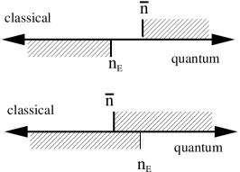
Figure 3: On the left down (up) is shown the case when (14) provides non-trivial (resp. trivial) bound on the metric entropy $H_{{\scriptscriptstyle\mathrm{KS}}}(T,\mu)$. On the right is depicted the tower for the map $T_{\{2,4,4\}}$.

7.2 Classical towers

In what follows we construct the tower dynamical system corresponding to the map $T:=T_{\{2,4,4\}}$ (as defined by eq. (28)). To this end let us double the original phase space and consider the set $\widetilde{I}:=I\times\{0,1\}$. We will referee to the sets $\widetilde{I}_{0}=\{(x,0),x\in I\}$, $\widetilde{I}_{1}=\{(x,1),x\in I\}$ as the first and second levels of the tower $\widetilde{I}=\widetilde{I}_{0}\cup\widetilde{I}_{1}$ respectively. The tower map $\widetilde{T}:\widetilde{I}\to\widetilde{I}$ is then defined by:

$$\widetilde{T}(x,\eta)=\left\{\begin{array}[]{rl}(\bar{T}(x),0)&\mbox{ if }\eta=0,x\in[1/2,1]\mbox{ or }\eta=1\mbox{ and any }x\\ (\bar{T}(x),1)&\mbox{ if }\eta=0,x\in[0,1/2]\end{array}\right.$$ (69)

where $\bar{T}:=T_{\{2,2\}}$ is the uniformly expanding map corresponding to $T$. Consider now the first return map $\widetilde{T}_{\widetilde{I}_{0}}$ on the set $\widetilde{I}_{0}$. It is then straightforward to see that the action of $\widetilde{T}_{\widetilde{I}_{0}}$ on $\widetilde{I}_{0}\cong I$ coincides with the action of $T$ on $I$. In other words, $T$ can be regarded as the first return map for the lowest level of the tower (see fig. 3).

Given an invariant measure $\mu$ for $T$ (equivalently for $\widetilde{T}_{\widetilde{I}_{0}}$) one can construct (using a standard procedure, see e.g., [24], [30]) the probability measure $\widetilde{\mu}$ which is invariant under the tower map $\widetilde{T}$. Precisely, for a set $A\subseteq I$ one defines the measures of the sets $(A\times\{0\})$, $(A\times\{1\})$ by

$$\widetilde{\mu}(A\times\{0\})=\Gamma^{-1}\mu(A),\qquad\widetilde{\mu}(A\times\{1\})=\Gamma^{-1}\mu(\bar{T}^{-1}A\cap[1/2,1]),$$

with the normalization constant $\Gamma=1+\mu([1/2,1])$. If $A=\llbracket\mathrm{x}\rrbracket$ is a cylinder set this can be rewritten as:

$$\widetilde{\mu}(\llbracket\mathrm{x}\rrbracket\times\{0\})=\Gamma^{-1}\mu(\llbracket\mathrm{x}\rrbracket),\qquad\widetilde{\mu}(\llbracket\mathrm{x}\rrbracket\times\{1\})=\Gamma^{-1}\mu(\llbracket 1\mathrm{x}\rrbracket).$$ (70)

Since $\widetilde{\mu}$ is invariant under $\widetilde{T}$ it makes sense to consider the corresponding metric entropy $H_{{\scriptscriptstyle\mathrm{KS}}}(\widetilde{T},\widetilde{\mu})$. An important observation is that $H_{{\scriptscriptstyle\mathrm{KS}}}(\widetilde{T},\widetilde{\mu})$ is related to $H_{{\scriptscriptstyle\mathrm{KS}}}(T,\mu)$. As $T$ is the first return map for $\widetilde{I}_{0}$, and $\mu(\widetilde{I}_{0})=\Gamma^{-1}$, by Abramov’s formula (see e.g., [24]) one gets:

$$H_{{\scriptscriptstyle\mathrm{KS}}}(T,\mu)=\Gamma H_{{\scriptscriptstyle\mathrm{KS}}}(\widetilde{T},\widetilde{\mu}).$$ (71)

Having an invariant measure $\widetilde{\mu}$ on $\widetilde{I}$ it is possible in turn to construct a measure $\bar{\mu}$ on $I$ which is invariant under the homogeneous map $\bar{T}$. Let $\boldsymbol{\pi}_{I}:\widetilde{I}\to I$ be a natural projection on the tower: $\boldsymbol{\pi}_{I}(x,\eta)=x$, for all $x\in I$, $\eta=\{0,1\}$. As

$$\boldsymbol{\pi}_{I}\circ\widetilde{T}=\bar{T}\circ\boldsymbol{\pi}_{I},$$

it follows immediately that the measure

$$\bar{\mu}:=\widetilde{\mu}\circ\boldsymbol{\pi}_{I}^{-1}$$ (72)

is invariant under $\bar{T}$. Furthermore, the metric entropy of $\bar{\mu}$ turns out to be equal to the metric entropy of $\widetilde{\mu}$:

$$H_{{\scriptscriptstyle\mathrm{KS}}}(\bar{T},\bar{\mu})=H_{{\scriptscriptstyle\mathrm{KS}}}(\widetilde{T},\widetilde{\mu}).$$ (73)

This equality can be deduced, from a version of the Abramov-Rokhlin relative entropy formula in [31]. For the sake of completeness we give a simple proof of (73) in the appendix of the paper.

The above construction allows a straightforward extension to the case of an arbitrary map of the form $T_{p}=T_{\mathbf{\Lambda}}$, where $\Lambda_{j}=p^{n_{j}},\,\,j=1,\dots l$ and $1<p\in\mathbbm{N}$. The tower phase space here is defined as $l_{\scriptscriptstyle\mathrm{tow}}:=\max_{j=1,\dots l}\{n_{j}\}$ copies of $I$:

$$\widetilde{I}=I\times\{0,1,\dots,l_{\scriptscriptstyle\mathrm{tow}}-1\}\cong\cup_{j=1}^{l-1}\widetilde{I_{j}},$$ (74)

where the set $\widetilde{I}_{j}=I\times\{j\}$ stands for $j$’s level of the tower. The tower map $\widetilde{T}_{p}:\widetilde{I}\to\widetilde{I}$ is then defined with the help of the uniformly expanding map $\bar{T}_{p}$ given by eq. (18). For each level $\eta\in\{0,1,\dots,l_{\scriptscriptstyle\mathrm{tow}}-1\}$ define the corresponding “jumping” set by

$$\mathcal{D}_{\eta}:=\cup_{\{j|n_{j}=\eta\}}I_{j},$$

then the action of the map $\widetilde{T}_{p}$ is given by:

$$\widetilde{T}_{p}(x,\eta)=\left\{\begin{array}[]{lr}(\bar{T}_{p}(x),0)&\mbox{ if }x\in\mathcal{D}_{\eta}\\ (\bar{T}_{p}(x),\eta+1)&\mbox{ if }x\not\in\mathcal{D}_{\eta}.\end{array}\right.$$ (75)

Such a definition implies that with each iteration a point in the tower phase space climbs one step upstairs up to the moment when it reaches at some level $\eta$ the set $\mathcal{D}_{\eta}$. Then it “jumps” downstare to zero level and the process is repeated.

It is now straightforward to see that the map $T_{p}$ coincides with the first return map of $\widetilde{T}_{p}$ for zero level $\widetilde{I}_{0}$ of the tower. As a result, starting from an invariant measure $\mu$ for $T_{p}$ one can easily construct the invariant measure $\widetilde{\mu}$ for the tower map $\widetilde{T}_{p}$. For a set $A\times\eta\subseteq\widetilde{I}$, with $A\subseteq I$ and level $\eta\in\{0,\dots l_{\scriptscriptstyle\mathrm{tow}}-1\}$ the corresponding measure is given by

$$\widetilde{\mu}(A\times\eta)=\Gamma^{-1}\sum_{\{k|n_{k}\geq\eta\}}\mu(\bar{T}^{-\eta}_{p}(A)\cap I_{k}),$$ (76)

where $\Gamma=\sum_{j=1}^{l}n_{j}\mu(I_{j})$ is the average return time to zero level of the tower. Precisely as for the map $T_{\{2,4,4\}}$, one can also construct the measure $\bar{\mu}$ invariant under the action of $\bar{T}_{p}$. The corresponding metric entropies are then related by:

$$H_{{\scriptscriptstyle\mathrm{KS}}}(T_{p},\mu)=\Gamma H_{{\scriptscriptstyle\mathrm{KS}}}(\bar{T}_{p},\bar{\mu})=\Gamma H_{{\scriptscriptstyle\mathrm{KS}}}(\widetilde{T}_{p},\widetilde{\mu}).$$ (77)

7.3 Quantum towers

We are going now to consider the quantum analog of the above tower construction.

Construction. Let $U=U_{\Bbbk}$ be a tensorial quantization of the map $T=T_{\{2,4,4\}}$, acting on the Hilbert space $\mathcal{H}=\mathcal{H}_{\Bbbk}$ of the dimension $2^{\Bbbk}=\mathrm{dim}(\mathcal{H}_{\Bbbk})$. We will assume that $U$ is of the form (29). In that case $U$ allows an obvious decomposition:

$$U=\bar{U}P_{\llbracket 0\rrbracket}+\bar{U}_{1}\bar{U}P_{\llbracket 1\rrbracket},$$ (78)

where $\bar{U}$ stands for a tensorial quantization of the uniformly expanding map $\bar{T}=T_{\{2,2\}}$ acting on the Hilbert space $\mathcal{H}$ and $\bar{U}_{1}=\sigma\bar{U}$ with the unitary $\sigma$ given by the exchange operation of the last two symbols in $|\mathrm{x}_{1}\rangle\otimes\dots\otimes|\mathrm{x}_{\Bbbk-1}\rangle\otimes|\mathrm{x}_{\Bbbk}\rangle\in\mathcal{H}$:

$$\sigma|\mathrm{x}_{1}\rangle\otimes\dots\otimes|\mathrm{x}_{\Bbbk-1}\rangle\otimes|\mathrm{x}_{\Bbbk}\rangle=|\mathrm{x}_{1}\rangle\otimes\dots\otimes|\mathrm{x}_{\Bbbk}\rangle\otimes|\mathrm{x}_{\Bbbk-1}\rangle.$$

In addition to $P_{\llbracket 0\rrbracket}$, $P_{\llbracket 1\rrbracket}$ it will be also convenient to use the projection operators:

$$P^{\prime}_{\llbracket 0\rrbracket}=\bar{U}P_{\llbracket 0\rrbracket}\bar{U}^{*},\qquad P^{\prime}_{\llbracket 1\rrbracket}=\bar{U}P_{\llbracket 1\rrbracket}\bar{U}^{*}.$$ (79)

Explicitly their action on the basis states of $\mathcal{H}$ is given by:

$$P^{\prime}_{\llbracket j\rrbracket}|\mathrm{x}_{1}\rangle\otimes\dots\otimes|\mathrm{x}_{\Bbbk-1}\rangle\otimes|\mathrm{x}_{\Bbbk}\rangle=|\mathrm{x}_{1}\rangle\otimes\dots\otimes|\mathrm{x}_{\Bbbk-1}\rangle\otimes\mathbf{U}\mathbf{P}_{j}\mathbf{U}^{*}|\mathrm{x}_{\Bbbk}\rangle,$$

where $\mathbf{P}_{j}|i\rangle=\delta_{i,j}|i\rangle$, $i,j\in\{0,1\}$. It worth to notice that $P^{\prime}_{\llbracket j\rrbracket}$’s commute with $\bar{U}_{1}$:

$$\bar{U}_{1}P^{\prime}_{\llbracket 1\rrbracket}=P^{\prime}_{\llbracket 1\rrbracket}\bar{U}_{1},\qquad\bar{U}_{1}P^{\prime}_{\llbracket 0\rrbracket}=P^{\prime}_{\llbracket 0\rrbracket}\bar{U}_{1}.$$ (80)

We define now the “tower” Hilbert space $\widetilde{\mathcal{H}}=\widetilde{\mathcal{H}}_{0}\oplus\widetilde{\mathcal{H}}_{1}$, $\mathrm{dim}(\widetilde{\mathcal{H}})=2^{\Bbbk}+2^{\Bbbk-1}$ with

$$\widetilde{\mathcal{H}}_{0}:=\mathcal{H},\mbox{ and }\widetilde{\mathcal{H}}_{1}:=\bar{U}P_{\llbracket 1\rrbracket}\mathcal{H}\equiv P^{\prime}_{\llbracket 1\rrbracket}\mathcal{H},$$ (81)

corresponding to zero and first levels of the tower. The scalar product on $\widetilde{\mathcal{H}}$ is defined in a standard way using the scalar product at each level. Namely for $\Phi=(\phi_{0},\phi_{1})\in\widetilde{\mathcal{H}}$, $\Phi^{\prime}=(\phi^{\prime}_{0},\phi^{\prime}_{1})\in\widetilde{\mathcal{H}}$, with $\phi_{0},\phi^{\prime}_{0}\in\widetilde{\mathcal{H}}_{0}$ and $\phi_{1},\phi^{\prime}_{1}\in\widetilde{\mathcal{H}}_{1}$:

$$\boldsymbol{(}\Phi,\Phi^{\prime}\boldsymbol{)}=\langle\phi_{0},\phi^{\prime}_{0}\rangle+\langle\phi_{1},\phi^{\prime}_{1}\rangle.$$

An orthonormal basis in $\widetilde{\mathcal{H}}$ can be easily constructed from an orthonormal basis in $\mathcal{H}$. A convenient choice is provided by the vectors:

$$\mathcal{E}_{(\mathrm{x},0)} :=(|\mathrm{x}_{1}\rangle\otimes\dots\otimes|\mathrm{x}_{\Bbbk-1}\rangle\otimes|\mathrm{x}_{\Bbbk}\rangle,\,0), \mathrm{x} =\mathrm{x}_{1}\dots\mathrm{x}_{\Bbbk-1}\mathrm{x}_{\Bbbk};$$

$$\mathcal{E}_{(\mathrm{x},1)} :=(0,\,|\mathrm{x}_{1}\rangle\otimes\dots\otimes|\mathrm{x}_{\Bbbk-1}\rangle\otimes|1^{\prime}\rangle), \mathrm{x} =\mathrm{x}_{1}\dots\mathrm{x}_{\Bbbk-2}\mathrm{x}_{\Bbbk-1},$$ (82)

where $|0^{\prime}\rangle:=\mathbf{U}|0\rangle$, $|1^{\prime}\rangle:=\mathbf{U}|1\rangle$ and $\mathrm{x}_{i}$, $i=1,\dots\Bbbk$ (resp. $i=1,\dots\Bbbk-1$) run over all possible sequences of $\{0,1\}$.

In what follows we will consider one-parameter family of tower evolution operators $\widetilde{U}_{\theta}:\widetilde{\mathcal{H}}\to\widetilde{\mathcal{H}}$ defined in the following way. For any $\Phi=(\phi_{0},\,\phi_{1})\in\widetilde{\mathcal{H}}$, with $\phi_{0}\in\widetilde{\mathcal{H}}_{0}$ and $\phi_{1}\in\widetilde{\mathcal{H}}_{1}$:

$$\widetilde{U}_{\theta}\Phi:=(\bar{U}_{1}P^{\prime}_{\llbracket 1\rrbracket}\phi_{1}+\bar{U}P_{\llbracket 0\rrbracket}\phi_{0},\,e^{i\theta}\bar{U}P_{\llbracket 1\rrbracket}\phi_{0}).$$ (83)

Correspondingly, the adjoint operation $\widetilde{U}_{\theta}^{*}:\widetilde{\mathcal{H}}\to\widetilde{\mathcal{H}}$ is given by:

$$\widetilde{U}^{*}_{\theta}\Phi=(e^{-i\theta}P_{\llbracket 1\rrbracket}\bar{U}^{*}\phi_{1}+P_{\llbracket 0\rrbracket}\bar{U}^{*}\phi_{0},\,P^{\prime}_{\llbracket 1\rrbracket}\bar{U}_{1}^{*}\phi_{0}).$$ (84)

Main properties. It is straightforward to see that $\widetilde{U}_{\theta}\,\Phi,\,\widetilde{U}_{\theta}^{*}\,\Phi\in\widetilde{\mathcal{H}}$ and $\widetilde{U}_{\theta}$ is a unitary operation on $\widetilde{\mathcal{H}}$:

Proposition 6.

Let $\widetilde{U}_{\theta},\widetilde{U}^{*}_{\theta}$ be as above, then

$$\widetilde{U}_{\theta}\,\widetilde{U}^{*}_{\theta}=\widetilde{U}_{\theta}^{*}\,\widetilde{U}_{\theta}=\mathbbm{1}.$$

Proof:

Straightforward calculation using eqs. (79, 80). $\Box$

Below we demonstrate that the Egorov property holds for $\widetilde{U}_{\theta}$. Specifically the short time evolution of projection operators is prescribed by the classical evolution of the corresponding tower map.

Proposition 7.

Let $\llbracket\mathrm{x}\rrbracket\subset I$ be a cylinder of the length $m=|\mathrm{x}|<\Bbbk-1$, then:

$$\widetilde{U}^{*}_{\theta}\,(P_{\llbracket\mathrm{x}\rrbracket}\oplus 0)\,\widetilde{U}_{\theta}=(P_{\llbracket 0\rrbracket}P_{\bar{T}^{-1}\llbracket\mathrm{x}\rrbracket}\oplus P^{\prime}_{\llbracket 1\rrbracket}P_{\bar{T}^{-1}\llbracket\mathrm{x}\rrbracket}),$$ (85)

$$\widetilde{U}^{*}_{\theta}\,(0\oplus P^{\prime}_{\llbracket 1\rrbracket}P_{\llbracket\mathrm{x}\rrbracket})\,\widetilde{U}_{\theta}=(P_{\llbracket 1\rrbracket}P_{\bar{T}^{-1}\llbracket\mathrm{x}\rrbracket}\oplus 0).$$ (86)

Proof:

In the matrix representation the left side of (85) reads as:

$$\left(\begin{array}[]{cc}P_{\llbracket 0\rrbracket}\bar{U}^{*}&e^{-i\theta}P_{\llbracket 1\rrbracket}\bar{U}^{*}\\ P^{\prime}_{\llbracket 1\rrbracket}\bar{U}_{1}^{*}&0\end{array}\right)\left(\begin{array}[]{cc}P_{\llbracket\mathrm{x}\rrbracket}&0\\ 0&0\end{array}\right)\left(\begin{array}[]{cc}\bar{U}P_{\llbracket 0\rrbracket}&\bar{U}_{1}P^{\prime}_{\llbracket 1\rrbracket}\\ e^{i\theta}\bar{U}P_{\llbracket 1\rrbracket}&0\end{array}\right).$$ (93)

By eqs. (79, 80) the off diagonal terms of the above product are zeros, and the diagonal part:

$$\left(\begin{array}[]{cc}P_{\llbracket 0\rrbracket}\bar{U}^{*}P_{\llbracket\mathrm{x}\rrbracket}\bar{U}P_{\llbracket 0\rrbracket}&0\\ 0&P^{\prime}_{\llbracket 1\rrbracket}\bar{U}_{1}^{*}P_{\llbracket\mathrm{x}\rrbracket}\bar{U}_{1}P^{\prime}_{\llbracket 1\rrbracket}\end{array}\right)$$

coincides with the right side of (85) by Corollary 38 and obvious equality: $\sigma P_{\llbracket\mathrm{x}\rrbracket}\sigma=P_{\llbracket\mathrm{x}\rrbracket}$. Eq. (86) is then proved analogously. $\Box$

Corollary 2.

Let $\widetilde{P}_{\bar{T}^{-n}\llbracket\mathrm{x}\rrbracket}=(P_{\bar{T}^{-n}\llbracket\mathrm{x}\rrbracket}\oplus P^{\prime}_{\llbracket 1\rrbracket}P_{\bar{T}^{-n}\llbracket\mathrm{x}\rrbracket})$ be the projection operator on the subset $(\bar{T}^{-n}\llbracket\mathrm{x}\rrbracket,0)\cup(0,\bar{T}^{-n}\llbracket\mathrm{x}\rrbracket)$, $|\mathrm{x}|=m$ of the tower. Then for all $n+m<\Bbbk-1$:

$$\widetilde{U}^{*}_{\theta}\,\widetilde{P}_{\bar{T}^{-n}\llbracket\mathrm{x}\rrbracket}\,\widetilde{U}_{\theta}=\widetilde{P}_{\bar{T}^{-n-1}\llbracket\mathrm{x}\rrbracket}.$$ (94)

Eigenfunctions and semiclassical measures. Given an eigenfunction $\psi$ of the original evolution operator $U$, $U\psi=e^{i\theta}\psi$ we can construct the eigenfunction of the tower evolution operator $\widetilde{U}_{\theta}$. Precisely, the state:

$$\Psi=(\psi,\bar{U}P_{\llbracket 1\rrbracket}\psi)/\Gamma_{\psi}^{1/2},\qquad\Gamma_{\psi}=1+\langle\psi,P_{\llbracket 1\rrbracket}\psi\rangle,$$ (95)

is the normalized eigenstate of the operator $\widetilde{U}_{\theta}$: $\widetilde{U}_{\theta}\Psi=e^{i\theta}\Psi$, $\boldsymbol{(}\Psi,\Psi\boldsymbol{)}=1$.

For any sequence of eigenstates $\{\psi_{\Bbbk}\}$ of quantizations $\{U_{\Bbbk}\}$ of $T$ one obtains applying (95) the corresponding sequence of the eigenstates $\{\Psi_{\Bbbk}\}$ of the quantizations $\{\widetilde{U}_{\theta_{\Bbbk}}\}$ of the tower map $\widetilde{T}$. As a result, a sequence of semiclassical measures $\mu_{\Bbbk}$ on $I$ induces the sequence of semiclassical measures $\widetilde{\mu}_{\Bbbk}$ on $\widetilde{I}$. For a cylinder $\llbracket\mathrm{x}\rrbracket\subset I$ the measures $\widetilde{\mu}_{\Bbbk}$ of the tower sets $\llbracket\mathrm{x}\rrbracket\times\{0\}$, $\llbracket\mathrm{x}\rrbracket\times\{1\}$ are defined as:

$$\widetilde{\mu}_{\Bbbk}(\llbracket\mathrm{x}\rrbracket\times\{0\})=\boldsymbol{(}\Psi_{\Bbbk},\,P_{\llbracket\mathrm{x}\rrbracket}\oplus 0\,\Psi_{\Bbbk}\boldsymbol{)},\qquad\widetilde{\mu}_{k}(\llbracket\mathrm{x}\rrbracket\times\{1\})=\boldsymbol{(}\Psi_{\Bbbk},\,0\oplus P_{\llbracket\mathrm{x}\rrbracket}\,\Psi_{\Bbbk}\boldsymbol{)}.$$

By eq. (95) these measures are related to the measure $\mu_{\Bbbk}$ of the set $\llbracket\mathrm{x}\rrbracket$:

$$\widetilde{\mu}_{\Bbbk}(\llbracket\mathrm{x}\rrbracket\times\{0\})=\Gamma^{-1}_{\Bbbk}{\mu}_{\Bbbk}(\llbracket\mathrm{x}\rrbracket),\qquad\widetilde{\mu}_{k}(\llbracket\mathrm{x}\rrbracket\times\{1\})=\Gamma^{-1}_{\Bbbk}{\mu}_{\Bbbk}(\llbracket 1\mathrm{x}\rrbracket),$$ (96)

where we set $\Gamma_{\Bbbk}=\Gamma_{\psi_{\Bbbk}}$. Note that after taking the limit $\Bbbk\to\infty$ in (96) one obtains eqs. (70), where $\widetilde{\mu}=\lim_{\Bbbk\to\infty}\widetilde{\mu}_{\Bbbk}$ is precisely the measure of the classical tower obtained from the semiclassical measure $\mu=\lim_{\Bbbk\to\infty}{\mu}_{\Bbbk}$ by the procedure from the previous section. Also, defining the measure $\bar{\mu}_{\Bbbk}$ on $I$ by

$$\bar{\mu}_{\Bbbk}(\llbracket\mathrm{x}\rrbracket):=\boldsymbol{(}\Psi_{\Bbbk},\widetilde{P}_{\llbracket\mathrm{x}\rrbracket}\Psi_{\Bbbk}\boldsymbol{)}=\Gamma^{-1}_{\Bbbk}\left({\mu}_{\Bbbk}(\llbracket\mathrm{x}\rrbracket)+{\mu}_{\Bbbk}(\llbracket 1\mathrm{x}\rrbracket)\right),$$ (97)

one reveals in the semiclassical limit the measure $\bar{\mu}=\lim_{\Bbbk\to\infty}\bar{\mu}_{\Bbbk}$ related to $\widetilde{\mu}$ by eq. (72).

We leave it to the reader to check that the above construction can be extended to all maps $T_{p}$.

7.4 Proof of Theorem 15

Let us now prove the bound (15) for the map $T_{2}$.

Theorem 8.

Let $\{U_{\Bbbk}\}_{\Bbbk=1}^{\infty}$ be a sequence of tensorial quantizations of $T=T_{\{2,4,4\}}$. For a sequence $\{\psi_{\Bbbk}\}_{\Bbbk=1}^{\infty}$ of eigenstates $U_{\Bbbk}\psi_{\Bbbk}=e^{i\theta_{\Bbbk}}\psi_{\Bbbk}$ let $\mu=\lim_{\Bbbk\to\infty}\mu_{\Bbbk}$ be the corresponding semiclassical measure, then:

$$H_{{\scriptscriptstyle\mathrm{KS}}}(T,\mu)\geq\frac{\mu(\llbracket 0\rrbracket)+2\mu(\llbracket 1\rrbracket)}{2}\log 2.$$ (98)

Proof:

To prove (98) it is possible, in principle, to follow precisely the scheme described in the beginning of the section i.e., to prove the bound on $H_{{\scriptscriptstyle\mathrm{KS}}}(\widetilde{T},\widetilde{\mu})$ for the corresponding semiclassical measure $\widetilde{\mu}$ on the tower and then deduce the bound (98) using Abramov’s formula. From the technical point of view, however, it turns out to be easier to prove an equivalent bound for the metric entropy $H_{{\scriptscriptstyle\mathrm{KS}}}(\bar{T},\bar{\mu})$ of the measure $\bar{\mu}$.

Let $\{\Psi_{\Bbbk}\}_{\Bbbk=1}^{\infty}$ be the sequence of the tower eigenstates corresponding to the sequence of $\psi_{\Bbbk}$’s, and let $\hat{h}_{n}(\Psi_{\Bbbk})\equiv h_{n}(\bar{\mu}_{\Bbbk})$ be the entropy function for the corresponding measures $\bar{\mu}_{\Bbbk}$:

$$h_{n}(\bar{\mu}_{\Bbbk})=-\sum_{|\mathrm{x}|=n}\bar{\mu}_{\Bbbk}(\llbracket\mathrm{x}\rrbracket)\log\bar{\mu}_{\Bbbk}(\llbracket\mathrm{x}\rrbracket)=-\sum_{|\mathrm{x}|=n}\|\widetilde{P}_{\llbracket\mathrm{x}\rrbracket}\Psi_{\Bbbk}\|^{2}\log(\|\widetilde{P}_{\llbracket\mathrm{x}\rrbracket}\Psi_{\Bbbk}\|^{2}).$$ (99)

Then the metric entropy $H_{{\scriptscriptstyle\mathrm{KS}}}(\bar{T},\bar{\mu})$ is obtained after first applying the semiclassical limit:

$$h_{n}(\bar{\mu})=\lim_{\Bbbk\to\infty}h_{n}(\bar{\mu}_{\Bbbk}).$$ (100)

and then the classical limit:

$$H_{{\scriptscriptstyle\mathrm{KS}}}(\bar{T},\bar{\mu})=\lim_{n\to\infty}\frac{1}{n}h_{n}(\bar{\mu}).$$ (101)

To prove the bound on $H_{{\scriptscriptstyle\mathrm{KS}}}(\bar{T},\bar{\mu})$ we will make use of the same scheme as in [16]. The first step is to get the bound on the entropy function, when $n$ is of of the same order as $\Bbbk$. This is provided by the following proposition.

Proposition 8.

Let $h_{n}(\bar{\mu}_{\Bbbk})$ be as in (99) and set $n=\Bbbk-1$, then

$$h_{\Bbbk-1}(\bar{\mu}_{\Bbbk})\geq\left(\frac{\Bbbk-1}{2}-1\right)\log 2.$$ (102)

Proof:

We will use the Uncertainty Entropic principle (Theorem 46) for the partitions: $\pi=\tau=\{\widetilde{P}_{\llbracket\mathrm{y}\rrbracket},\,\,|\mathrm{y}|=\Bbbk-1\}$, weights: $v_{\mathrm{y}}=w_{\mathrm{y}}\equiv 1$ and isometry operation $\mathcal{U}=(\widetilde{U}_{\theta_{\Bbbk}})^{\Bbbk-1}$. Since $\Psi_{\Bbbk}$ is an eigenstate of $\widetilde{U}_{\theta_{\Bbbk}}$ it follows immediately from (46):

$$h_{\Bbbk-1}(\Psi_{\Bbbk})\geq-\log(\sup_{|\mathrm{y}|=|\mathrm{y}^{\prime}|=\Bbbk-1}\|\widetilde{P}_{\llbracket\mathrm{y}\rrbracket}(\widetilde{U}_{\theta_{\Bbbk}})^{\Bbbk-1}\widetilde{P}_{\llbracket\mathrm{y}^{\prime}\rrbracket}\|).$$ (103)

Thus one needs to estimate the norm of the matrix $\mathcal{C}(\mathrm{y},\mathrm{y}^{\prime})=\widetilde{P}_{\llbracket\mathrm{y}\rrbracket}(\widetilde{U}_{\theta_{\Bbbk}})^{\Bbbk-1}\widetilde{P}_{\llbracket\mathrm{y}^{\prime}\rrbracket}$. To this end let us calculate the matrix elements of $\mathcal{C}(\mathrm{y},\mathrm{y}^{\prime})$:

$$\boldsymbol{(}\mathcal{E}_{(\mathrm{x},i)},\mathcal{C}(\mathrm{y},\mathrm{y}^{\prime})\mathcal{E}_{(\mathrm{x}^{\prime},i^{\prime})}\boldsymbol{)},$$

in the basis of orthogonal states (82) with the parameters: $i,i^{\prime}\in\{0,1\}$, $|\mathrm{x}|=\Bbbk-1$, ($|\mathrm{x}^{\prime}|=\Bbbk-1$) if $i=0$ (resp. $i^{\prime}=0$) and $|\mathrm{x}|=\Bbbk$, ($|\mathrm{x}^{\prime}|=\Bbbk$) if $i=1$ (resp. $i^{\prime}=1$). The action of the projection operator on the basis states is given by

$$\widetilde{P}_{\llbracket\mathrm{y}\rrbracket}\mathcal{E}_{(\mathrm{x},i)}=\mathcal{E}_{(\mathrm{x},i)}\left(\prod_{m=1}^{\Bbbk-1}\delta_{\mathrm{x}_{m},\mathrm{y}_{m}}\right).$$ (104)

Hence for each pair of $\mathrm{y},\mathrm{y}^{\prime}$ there exist at most two values of $\mathrm{x}$ and two values of $\mathrm{x}^{\prime}$ such that the matrix elements $\boldsymbol{(}\mathcal{E}_{(\mathrm{x},i)},\mathcal{C}(\mathrm{y},\mathrm{y}^{\prime})\mathcal{E}_{(\mathrm{x}^{\prime},i^{\prime})}\boldsymbol{)}$ are not zeros. From that follows:

$$\|\mathcal{C}(\mathrm{y},\mathrm{y}^{\prime})\|\leq 2\max_{(\mathrm{x},i),(\mathrm{x}^{\prime},i^{\prime})}|\boldsymbol{(}\mathcal{E}_{(\mathrm{x},i)},\mathcal{C}(\mathrm{y},\mathrm{y}^{\prime})\mathcal{E}_{(\mathrm{x}^{\prime},i^{\prime})}\boldsymbol{)}|=2\max_{(\mathrm{x},i),(\mathrm{x}^{\prime},i^{\prime})}|\boldsymbol{(}\mathcal{E}_{(\mathrm{x},i)},(\widetilde{U}_{\theta_{\Bbbk}})^{\Bbbk-1}\mathcal{E}_{(\mathrm{x}^{\prime},i^{\prime})}\boldsymbol{)}|.$$ (105)

Therefore, it remains to estimate the elements of the operator $(\widetilde{U}_{\theta_{\Bbbk}})^{\Bbbk-1}$ in the basis of $\{\mathcal{E}_{(\mathrm{x},i)}\}$. To this end, let us notice that the action of $\widetilde{U}_{\theta_{\Bbbk}}$ on $\{\mathcal{E}_{(\mathrm{x},i)}\}$ up to times $\Bbbk$ closely connected to the action of the corresponding tower map $\widetilde{T}$ on the sets $\llbracket\mathrm{x}\rrbracket\times\{i\}$ of $\widetilde{I}$. Specifically, let $\mathcal{E}=(\widetilde{U}_{\theta_{\Bbbk}})^{\Bbbk-1}\mathcal{E}_{(\mathrm{x},i)}$. Then, as follows from eq. (83), depending on $\mathrm{x}$, $i$ the state $\mathcal{E}$ might take the values $(e,0)$ or $(0,e)$, where

$$e=e^{iQ\theta_{\Bbbk}}|\mathrm{x}^{\prime}_{\Bbbk}\rangle\otimes\mathbf{U}|\mathrm{x}_{i_{1}}\rangle\otimes\mathbf{U}|\mathrm{x}_{i_{2}}\rangle\otimes\dots\otimes\mathbf{U}|\mathrm{x}_{i_{\Bbbk-1}}\rangle.$$ (106)

Here $\mathrm{x}_{i_{1}},\mathrm{x}_{i_{2}}\dots\mathrm{x}_{i_{\Bbbk-1}}$ is some permutation of the original sequence $\mathrm{x}_{1},\mathrm{x}_{2}\dots\mathrm{x}_{\Bbbk-1}$ and $Q$ is an integer number. Since $|\langle\mathrm{x}_{j},\mathbf{U}\mathrm{x}_{i}\rangle|=1/\sqrt{2}$ for any pair $\mathrm{x}_{i},\mathrm{x}_{j}\in\{0,1\}$,

$$|\boldsymbol{(}\mathcal{E}_{(\mathrm{x}^{\prime},i^{\prime})},(\widetilde{U}_{\theta_{\Bbbk}})^{\Bbbk-1}\mathcal{E}_{(\mathrm{x},i)}\boldsymbol{)}|=|\boldsymbol{(}\mathcal{E}_{(\mathrm{x}^{\prime},i^{\prime})},\mathcal{E}\boldsymbol{)}|\leq 2^{-\left(\frac{\Bbbk-1}{2}\right)}.$$

Together with (103) and (105) this gives the proof of the proposition. $\Box$

The second necessary step is to connect values $h_{\Bbbk-1}(\bar{\mu}_{\Bbbk})$ of the entropy at quantum times of order $\Bbbk$ to its values $h_{n}(\bar{\mu}_{\Bbbk})$ at short fixed classical times $n$.

Proposition 9.

Let $h_{n}(\bar{\mu}_{\Bbbk})$ be as in (99), and let $\Bbbk-1=qn+r$, $r\leq n$ where $n<\Bbbk-1$ is a fixed (classical) time and $q$, $r$ are integers, then

$$\frac{1}{n}h_{n}(\bar{\mu}_{\Bbbk})\geq\frac{1}{\Bbbk-1}h_{\Bbbk-1}(\bar{\mu}_{\Bbbk})-\frac{n\log 2}{\Bbbk-1}.$$ (107)

Proof:

To prove (107) one makes use of the fact that the measure $\bar{\mu}_{\Bbbk}$ is invariant under the transformation $\bar{T}^{j}$ up to certain times $j$. From the definition of $\bar{\mu}_{\Bbbk}$ and eq. (38) it follows that for any cylinder $\llbracket\mathrm{x}\rrbracket$ of a length $|\mathrm{x}|=m$:

$$\bar{\mu}_{\Bbbk}(\llbracket\mathrm{x}\rrbracket)=\bar{\mu}_{\Bbbk}(\bar{T}^{-n}\llbracket\mathrm{x}\rrbracket),\mbox{ for }m+n\leq\Bbbk-1.$$ (108)

Let $n,q,r$ be as in the conditions of the proposition. Then the subadditivity property (40) of the entropy function implies

$$h_{\Bbbk-1}(\bar{\mu}_{\Bbbk})\leq-\sum_{j=0}^{q-1}\sum_{|\mathrm{x}|=n}\bar{\mu}_{\Bbbk}(\bar{T}^{-jn}\llbracket\mathrm{x}\rrbracket)\log\bar{\mu}_{\Bbbk}(\bar{T}^{-jn}\llbracket\mathrm{x}\rrbracket)-\sum_{|\mathrm{x}|=r}\bar{\mu}_{\Bbbk}(\bar{T}^{-qn}\llbracket\mathrm{x}\rrbracket)\log\bar{\mu}_{\Bbbk}(\bar{T}^{-qn}\llbracket\mathrm{x}\rrbracket),$$

and by eq. (108) this reads as

$$h_{\Bbbk-1}(\bar{\mu}_{\Bbbk})\leq qh_{n}(\bar{\mu}_{\Bbbk})+h_{r}(\bar{\mu}_{\Bbbk}).$$ (109)

Since $|h_{r}(\bar{\mu}_{\Bbbk})|$ is bounded from above by $n\log 2$ one gets immediately the inequality (107). $\Box$

End of the proof of Theorem 98: The final step is to combine Propositions 102 and 107:

$$\frac{1}{n}h_{n}(\bar{\mu}_{\Bbbk})\geq\frac{\log 2}{2}-\frac{(n+1)\log 2}{\Bbbk-1},\mbox{ for all }n<\Bbbk.$$ (110)

Taking in (110) first limit $\Bbbk\to\infty$ and then $n\to\infty$ gives:

$$H_{{\scriptscriptstyle\mathrm{KS}}}(\bar{T},\bar{\mu})\geq\frac{\log 2}{2},$$

which by (73, 71) implies the bound:

$$H_{{\scriptscriptstyle\mathrm{KS}}}({T},\mu)\geq\frac{\Gamma\log 2}{2}.$$ (111)

Since $\Gamma=\mu(\llbracket 0\rrbracket)+2\mu(\llbracket 1\rrbracket)$ this gives the bound (98). $\Box$

Theorem 98 can be straightforwardly generalized to other one-dimensional maps with slopes given by powers of the same integer.

Scetch of proof of Theorem 15:

All the ingredients of the above construction can be straightforwardly extended from the map $T_{\{2,4,4\}}$ to a general map $T_{p}$. In particular, starting from an invariant semiclassical measure $\mu$ of $T_{p}$ one can construct the invariant semiclassical measure $\widetilde{\mu}$ of the corresponding tower map $\widetilde{T}_{p}$ and the invariant semiclassical measure $\bar{\mu}$ of the corresponding uniformly expanding map $\bar{T}_{\Lambda}$. Repeating then all the previous steps of the present section one can show the bound:

$$H_{{\scriptscriptstyle\mathrm{KS}}}(\bar{T}_{p},\bar{\mu})\geq\frac{\log p}{2}.$$

Since the metric entropies $H_{{\scriptscriptstyle\mathrm{KS}}}(\bar{T}_{p},\bar{\mu}),H_{{\scriptscriptstyle\mathrm{KS}}}(\widetilde{T}_{p},\widetilde{\mu}),H_{{\scriptscriptstyle\mathrm{KS}}}({T}_{p},{\mu})$ are connected to each other one immediately gets

$$H_{{\scriptscriptstyle\mathrm{KS}}}(T_{p},\mu)\geq\Gamma\frac{\log p}{2},$$ (112)

where $\Gamma$ is the measure $\mu$ of the tower. Finally, it remains to check that $\Gamma$ gives the correct prefactor. $\Box$

8 Explicit sequences of “non-ergodic” eigenstates

Below we construct some explicit sequences of eigenstates for maps $\bar{T}_{p}$, $T_{p}$ quantized as in Section 3.2. Having such sequences we can calculate the induced semiclassical measures and test the bound (15) for the corresponding metric entropies.

8.1 Maps with uniform slopes

Let us first consider the map $\bar{T}_{p}$ with the uniform slope $p$ whose quantization is given by eq. (22). Note that if $\mathbf{U}$ is given by the discrete Fourier transform matrix, the evolution operator $\bar{U}_{\Bbbk}$ and the corresponding eigenstates are precisely the same as for Walsh-quantized baker’s map treated in [16]. For a general $\mathbf{U}$ the construction can be carried out in an analogous way. Let $w\in\mathcal{H}$ be an eigenstate of $\mathbf{U}$, then

$$\psi^{(w)}_{\Bbbk}=\underbrace{w\otimes w\otimes\dots w}_{\Bbbk},\qquad\psi^{(w)}_{\Bbbk}\in\mathcal{H}_{\Bbbk}$$ (113)

is the eigenstate of $\bar{U}_{\Bbbk}$. The semiclassical measure $\mu_{w}$ corresponding to the sequence $\psi^{(w)}_{\Bbbk}$, $\Bbbk=1,\dots\infty$ and the associated metric entropy of $\mu_{w}$ can be then easily calculated. Assuming that $w=\sum_{i=0}^{p-1}w_{i}|i\rangle$, where $\{|i\rangle,i=0,\dots p-1\}$ is an orthonormal basis in $\mathcal{H}$, the $\mu_{w}$-measure of the cylinder set $\llbracket\mathrm{x}\rrbracket$, $\mathrm{x}=\mathrm{x}_{1}\dots\mathrm{x}_{m}$ is given by:

$$\mu_{w}(\llbracket\mathrm{x}\rrbracket)=\lim_{\Bbbk\to\infty}\langle\psi_{\Bbbk}^{(w)}P_{\llbracket\mathrm{x}\rrbracket}\psi_{\Bbbk}^{(w)}\rangle=\prod_{i=1}^{m}|w_{\mathrm{x}_{i}}|^{2}.$$ (114)

As this is the product measure, one gets for the metric entropy:

$$H_{{\scriptscriptstyle\mathrm{KS}}}(\bar{T}_{p},\mu_{w})=-\sum_{i=0}^{p-1}|w_{i}|^{2}\log(|w_{i}|^{2}).$$ (115)

A more general class of eigenstates can be constructed by taking a set of states $\mathbf{w}:=\{w^{(j)}\in\mathcal{H},j=0,\dots d-1\}$ cyclically related to each other: $\mathbf{U}w^{(j)}=w^{(j+1\mod d)}$. Now define $\mathbf{w}_{0}:=w^{(0)}\otimes w^{(1)}\dots\otimes w^{(d-1)}$ and let $\mathbf{w}_{1},\mathbf{w}_{2},\dots\mathbf{w}_{d-1}$ be the vectors obtained from $\mathbf{w}_{0}$ by cyclic permutation of its components, e.g.,

$$\mathbf{w}_{i}:=w^{(i\mod d)}\otimes w^{(1+i\mod d)}\dots\otimes w^{(d-1+i\!\mod d)},\qquad i=0,\dots d-1.$$

For each $\Bbbk$ satisfying $\Bbbk\!\!\mod d=0$ one looks for eigenstates of $\bar{U}_{\Bbbk}$ in the form

$$\psi_{\Bbbk}^{(\mathbf{w})}=\sum_{i=0}^{d-1}\mathcal{C}^{(\Bbbk)}_{i}\,\underbrace{\mathbf{w}_{i}\otimes\mathbf{w}_{i}\otimes\dots\mathbf{w}_{i}}_{\Bbbk/d},\qquad\psi_{\Bbbk}^{(\mathbf{w})}\in\mathcal{H}_{\Bbbk}.$$ (116)

The normalization condition $\|\psi_{\Bbbk}^{(\mathbf{w})}\|=1$ implies:

$$\sum_{i=0}^{d-1}\left(\mathcal{C}_{i}\right)^{2}=1,\qquad\mathcal{C}_{i}=\lim_{\Bbbk\to\infty}|\mathcal{C}^{(\Bbbk)}_{i}|.$$

When all $\mathcal{C}^{(\Bbbk)}_{i}$ are equal, one gets by (116) the eigenstate of $\bar{U}_{\Bbbk}$ . (Note that the eigenstates (113) could be seen as a particular case of (116) when $d=1$.) The corresponding semiclassical measure is then given by the sum of the product measures

$$\mu_{\mathbf{w}}(\llbracket\mathrm{x}\rrbracket)=\lim_{\Bbbk\to\infty}\langle\psi_{\Bbbk}^{(\mathbf{w})}P_{\llbracket\mathrm{x}\rrbracket}\psi_{\Bbbk}^{(\mathbf{w})}\rangle=\sum_{i=0}^{d-1}(\mathcal{C}_{i})^{2}\mu^{(i)}_{\mathbf{w}}(\llbracket\mathrm{x}\rrbracket),$$

$$\mu^{(i)}_{\mathbf{w}}(\llbracket\mathrm{x}\rrbracket)=\prod_{j=1}^{m}|w^{(i+j-1\!\!\!\mod d)}_{\mathrm{x}_{j}}|^{2},$$ (117)

where $w^{(j)}_{i}$ is $i$’s component of the vector $w^{(j)}$ in the basis $\{|i\rangle,i=0,\dots p-1\}$. Although $\mu_{\mathbf{w}}$ is not a simple product measure, it is still possible to calculate the metric entropy explicitly:

$$H_{{\scriptscriptstyle\mathrm{KS}}}(\bar{T}_{p},\mu_{\mathbf{w}})=-\sum_{i=0}^{d-1}\sum_{j=0}^{p-1}|w^{(i)}_{j}|^{2}\log(|w^{(i)}_{j}|^{2}).$$ (118)

From a simple application of Uncertainty Entropic Principle it follows that $H_{{\scriptscriptstyle\mathrm{KS}}}(\bar{T}_{p},\mu_{w})\geq\frac{1}{2}\log p$ which is precisely the bound (14) (equivalent to (15) in that case). Furthermore, for $\mathbf{U}$ given by the discrete Fourier transform and $d=1$ there exist vectors $w$ such that measures $\mu_{w}$ saturate the above bound [16].

Note that if all $w^{(i)}_{j}\neq 0$ the measures above are supported on the whole $I$. As has been shown in [16] in the case when $\mathbf{U}$ is the discrete Fourier transform matrices, it is also possible to construct an entirely different class of exceptional sequences of eigenstates where parts of the corresponding semiclassical measures are localized on the periodic trajectories. This is due to the fact that when $\mathbf{U}^{n}=\mathbbm{1}$ for some small integer $n$, the spectrum of $\bar{U}_{\Bbbk}$ becomes highly degenerate. Since no such degeneracies are expected for quantized maps with non-uniform slopes, it seems that this type of semiclassical measures can be constructed only for the maps $\bar{T}_{p}$. We refer the reader to [16], [14] for the details of the construction.

8.2 Maps with non-uniform slope

For maps $T_{p}$ we will look for sequences of eigenstates having exactly the same form (116, 116) as for the uniform case. As we show, one can construct such sequences by choosing the matrices $\mathbf{U}_{i}$ and the constants $\mathcal{C}^{(\Bbbk)}_{i}$ in an appropriate way. Below we give several concrete examples of such a construction for the map (28) whose quantization is given by (29).

Example 1. Let $\mathbf{U}_{1}=\mathbf{U}_{2}=\mathbf{U}$ be two by two matrix satisfying $\mathbf{U}^{2}=-\mathbbm{1}$, $|\mathbf{U}(i,j)|=1/\sqrt{2}$, e.g., discrete Fourier transform. Let $\mathbf{U}|1\rangle=:|e_{+}\rangle$. Since $\mathbf{U}|e_{+}\rangle=-|1\rangle$ it can be easily seen that for even $\Bbbk$

$$\psi_{\Bbbk}^{(1)}=\underbrace{|1\rangle\otimes|e_{+}\rangle\dots|1\rangle\otimes|e_{+}\rangle}_{\Bbbk}$$ (119)

is an eigenstate of $U_{\Bbbk}$. For the sequence of states $\psi_{\Bbbk}^{(1)}$ the induced semiclassical measure $\mu_{\Bbbk}^{(1)}$ has entire support at the Cantor set. The metric entropy for this measure can be easily calculated: $H_{{\scriptscriptstyle\mathrm{KS}}}(T_{2},\mu^{(1)}_{\Bbbk})=\log 2$. Note that $H_{{\scriptscriptstyle\mathrm{KS}}}(T_{2},\mu^{(1)}_{\Bbbk})$ saturates the bound (15) which in that case coincides with (14).

Example 2. For the same map $T_{2}$ consider a slightly different quantization. Let $\mathbf{U}$ be an arbitrary unitary matrix whose elements have modules $1/\sqrt{2}$ and let $w$ be one of its eigenvectors with the eigenvalue $e^{i\gamma}$. We now fix $\mathbf{U}_{1}$, $\mathbf{U}_{2}$ by the conditions $\mathbf{U}_{2}=e^{-i\gamma}\mathbf{U}$, $\mathbf{U}_{1}=\mathbf{U}$. The state

$$\psi_{\Bbbk}^{(2)}=\underbrace{w\otimes w\otimes\dots w}_{\Bbbk},$$

is then the eigenstate of $U_{\Bbbk}$. Denote $\mu^{(2)}_{w}$ the corresponding semiclassical measure. Unlike the previous example, in general, $\mu^{(2)}_{w}$ is supported over all $I$. For a given state $w=w_{0}|0\rangle+w_{1}|1\rangle$ the measures of the sets $\llbracket\varepsilon_{0}\rrbracket,\varepsilon_{0}=\{1,2,3\}$ are:

$$\mu^{(2)}_{w}(\llbracket\varepsilon_{0}\rrbracket)=\lim_{\Bbbk\to\infty}\langle\psi_{\Bbbk}^{(2)}P_{\varepsilon_{0}}\psi_{\Bbbk}^{(2)}\rangle=\left\{\begin{array}[]{ll}p&\mbox{ for }\varepsilon_{0}=1\\ pq&\mbox{ for }\varepsilon_{0}=2\\ q^{2}&\mbox{ for }\varepsilon_{0}=3,\\ \end{array}\right.$$

where $|w_{0}|^{2}=p$, $|w_{1}|^{2}=q$. Since $\mu^{(2)}_{w}$ is a product measure the corresponding metric entropy is given by:

$$H_{{\scriptscriptstyle\mathrm{KS}}}(T_{2},\mu^{(2)}_{w})=-\sum_{\varepsilon_{0}=\{1,2,3\}}\mu^{(2)}_{w}(\llbracket\varepsilon_{0}\rrbracket)\log\mu^{(2)}_{w}(\llbracket\varepsilon_{0}\rrbracket)=-(p\log p+pq\log(pq)+q^{2}\log q^{2}).$$

Recall that $w$ is an eigenvector of a unitary matrix whose entries have the same modules. This restricts the possible values of $q$, $p=1-q$ to the interval $[(2-\sqrt{2})/4,(2+\sqrt{2})/4]$. As can be easily checked for all values of $q,p$ in this interval the strict inequality (15) holds. It worth to notice that this example allows straightforward generalization to all maps $T_{p}$.

Example 3. It is also possible to construct eigenstates of $U_{\Bbbk}$ using two state products:

$$\psi_{\Bbbk}^{(3)} = \mathcal{C}^{(\Bbbk)}_{1}\underbrace{w^{(1)}\otimes w^{(2)}\otimes w^{(1)}\otimes w^{(2)}\dots w^{(1)}\otimes w^{(2)}}_{\Bbbk}$$

$$+ \mathcal{C}^{(\Bbbk)}_{2}\underbrace{w^{(2)}\otimes w^{(1)}\otimes w^{(2)}\otimes w^{(1)}\dots w^{(2)}\otimes w^{(1)}}_{\Bbbk}.$$

Take

$$\mathbf{U}_{2}=\mathbf{U}_{1}=\mathbf{U},\qquad\mathbf{U}=\frac{1}{\sqrt{2}}\left(\begin{array}[]{cc}1&e^{i\alpha}\\ e^{-i\alpha}&-1\end{array}\right),\qquad(\mathbf{U})^{2}=\mathbbm{1}.$$

and set $\mathcal{C}^{(\Bbbk)}_{1}=z\mathcal{C}^{(\Bbbk)}_{2}$, $c=1+|z\sqrt{2}-1|^{2}$,

$$w^{(1)}=c^{-1/2}\left(|0\rangle+e^{-i\alpha}(z\sqrt{2}-1)|1\rangle\right),\qquad w^{(2)}=c^{-1/2}\left(z|0\rangle+e^{-i\alpha}(\sqrt{2}-z)|1\rangle\right).$$

It is easy to check that $\psi_{\Bbbk}^{(3)}$ is the eigenstate of $U_{\Bbbk}$ for any $z\in\mathbbm{C}$. The resulting semiclassical measure $\mu_{z}^{(3)}$ is the sum of two product measures (defined by eq. (117)). Note that $\mu_{z}^{(3)}$ is symmetric under the inversion $z\to z^{-1}$. Denote $p_{1,2}=|w^{(1,2)}_{2}|^{2}$, $q_{1,2}=|w^{(1,2)}_{1}|^{2}$. As will be shown in the rest of the section, the metric entropy of $\mu_{z}^{(3)}$ can be explicitly calculated and it is given by

$$H_{{\scriptscriptstyle\mathrm{KS}}}({T_{2},\mu_{z}^{(3)}})=-\frac{\Gamma}{2}\sum_{k=1,2}p_{k}\log p_{k}+q_{k}\log q_{k},$$

where

$$\Gamma=2(\mu([10])+\mu([11]))+\mu([0])=1+\mathcal{C}_{1}p_{1}+\mathcal{C}_{2}p_{2}.$$

The plot in fig. 4 shows both the metric entropy and the bound (15): $\frac{\Gamma}{2}\log 2$ as functions of the real part of $z$ for $\mathrm{Im}(z)=0$.

Some special cases: 1) $|z|=1$. In this case $p_{1}=p_{2}$, $q_{1}=q_{2}$ and the resulting measures of the simple product type. Furthermore, both $w^{(1)}$ and $w^{(2)}$ are the eigenvectors of the same unitary matrix whose elements have equal modulus. Thus one actually, gets the measures of the same type as for one vector product states $\psi_{\Bbbk}^{(2)}$ in the previous example. 2) $z=0,z=\infty$. In that case either $\mathcal{C}_{2}$ or $\mathcal{C}_{1}$ vanishes and we get the states considered in Example 1. 3) $z=\sqrt{2},z^{-1}=\sqrt{2}$. In such a case $p_{1}=q_{1}=1/2$, $p_{2}=0,q_{2}=1$ and the metric entropy $H_{{\scriptscriptstyle\mathrm{KS}}}({T_{2},\mu_{\scriptscriptstyle{\sqrt{2}}}^{(3)}})=\frac{2}{3}\log 2$ saturates the bound.

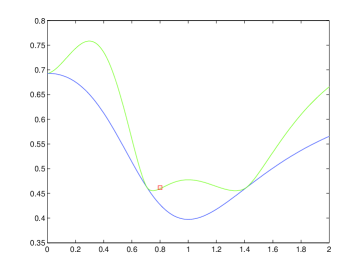
Figure 4: Metric entropy (green) and the corresponding bound (blue) (15) for the semiclassical measure in Example 3 as function of $\mathrm{Re}(z)$ when $\mathrm{Im}(z)=0$.

The above examples can be generalized to other maps $T_{p}$ to construct d-state product eigenstates of the type (116). More specifically, assume that by an appropriate choice of constants $\mathcal{C}^{(\Bbbk)}_{i}$ in one can construct an eigenstate $\psi_{\Bbbk}^{(\mathbf{w})}$ of the quantum evolution operator $U_{\Bbbk}$ (27) with $\mathbf{U}_{i}=\mathbf{U}$, for all $i$. It is instructive to see how the metric entropy of the corresponding semiclassical measures $\mu_{\mathbf{w}}$ can be calculated in general case.

Note that $\psi_{\Bbbk}^{(\mathbf{w})}$ being an eigenstate of $U_{\Bbbk}$, is in addition, an eigenstate for the operator $(\bar{U}_{\Bbbk})^{d}$, where $\bar{U}_{\Bbbk}$ is the quantization (22) of the map $\bar{T}_{p}$ with the uniform slope $p$. Since $(\bar{U}_{\Bbbk})^{d}$ is also a quantization of the map $\bar{T}_{p^{d}}$, the semiclassical measure $\mu_{\mathbf{w}}$ turns out to be invariant both for $T_{p}$ and $\bar{T}_{p^{d}}$ maps. The corresponding metric entropies $H_{{\scriptscriptstyle\mathrm{KS}}}(T_{p},\mu_{\mathbf{w}})$ and $H_{{\scriptscriptstyle\mathrm{KS}}}(\bar{T}_{p^{d}},\mu_{\mathbf{w}})$ can be connected to each other in the following way. Using either $T_{p}$ or $\bar{T}_{p}$ and the corresponding dynamically generated partitions, one can encode any point $\zeta\in I$ according to its dynamical “history“ in a two-fold way. The ”history“ with respect to $T_{p}$ and $\bar{T}_{p}$ are given by the sequences $\varepsilon(\zeta)=\varepsilon_{0}\varepsilon_{1}\dots$, $\varepsilon_{i}\in\{1,\dots l\}$ and $\mathrm{x}(\zeta)=\mathrm{x}_{1}\mathrm{x}_{2}\dots$, $\mathrm{x}_{i}\in\{0,\dots p-1\}$ respectively. Furthermore, each of these sequences generates the set of cylinders: $\{\llbracket\varepsilon_{0}\dots\varepsilon_{n}\rrbracket,n=0,1,\dots\}$, $\{\llbracket\mathrm{x}_{1}\dots\mathrm{x}_{n}\rrbracket,n=1,2,\dots\}$ corresponding to the ”partial histories“ of the point evolution with regards to $T_{p}$ and $\bar{T}_{p}$ respectively. The Shannon-McMillan-Breiman theorem asserts then that for almost every (with respect to $\mu_{\mathbf{w}}$) $\zeta\in I$ the metric entropy of $T_{p}$ is given by:

$$H_{{\scriptscriptstyle\mathrm{KS}}}(T_{p},\mu_{\mathbf{w}})=-\lim_{n\to\infty}\frac{1}{n}\log\mu_{\mathbf{w}}(\llbracket\varepsilon_{0}\dots\varepsilon_{n}\rrbracket).$$ (120)

Analogously, using the second representation for the same point $\zeta$ one gets:

$$\frac{1}{d}H_{{\scriptscriptstyle\mathrm{KS}}}(\bar{T}_{p^{d}},\mu_{\mathbf{w}})=-\lim_{n\to\infty}\frac{1}{n}\mu_{\mathbf{w}}(\llbracket\mathrm{x}_{1}\dots\mathrm{x}_{n}\rrbracket).$$ (121)

Thus the connection between two entropies is given by:

$$H_{{\scriptscriptstyle\mathrm{KS}}}(T_{p},\mu_{\mathbf{w}})=\frac{\Gamma}{d}H_{{\scriptscriptstyle\mathrm{KS}}}(\bar{T}_{p^{d}},\mu_{\mathbf{w}}).$$ (122)

The coefficient $\Gamma$ is defined by the limit:

$$\Gamma=\lim_{n\to\infty}m_{n}/n,$$

where $n$ is the length of the cylinder $G_{n}=\llbracket\varepsilon_{0}\dots\varepsilon_{n-1}\rrbracket$ in $\varepsilon$-representation and $m_{n}$ is the length of the same set $G_{n}=\llbracket\mathrm{x}_{1}\dots\mathrm{x}_{m_{n}}\rrbracket$ in the $\mathrm{x}$-representation. By the Birkhoff’s ergodic theorem this limit is equal to:

$$\Gamma=\sum_{i=1}^{l}q_{i}\mu_{\mathbf{w}}(I_{i}).$$ (123)

The formula for the metric entropy of $H_{{\scriptscriptstyle\mathrm{KS}}}(T_{p},\mu_{\mathbf{w}})$ is then follows immediately from (122) and the metric entropy (118) of the “homogeneous” map $\bar{T}_{p^{d}}$. Note also that as the right side of (15) amounts to $\Gamma\frac{\log p}{2}$ the proof of the Anantharaman-Nonnenmacher conjecture for the measure $\mu_{\mathbf{w}}$ amounts to the proof of

$$H_{{\scriptscriptstyle\mathrm{KS}}}(\bar{T}_{p^{d}},\mu_{\mathbf{w}})\geq\frac{\log p^{d}}{2}$$

for the uniformly expanding map $\bar{T}_{p^{d}}$.

9 Conclusions and outlook

In the current paper we proved Anantharaman-Nonnenmacher conjecture for a class of ”tensorial” quantizations of one-dimensional piecewise linear maps $T_{p}$ whose all slopes are powers of the same integer $p$. It should be stated that we deal here with ”tensorial” quantization mostly for the sake of convenience, as these quantizations allow very explicit treatment. Actually we believe that the current method with minimal adjustments can be used to prove the result for all quantizations of maps $T_{p}$. On the other hand, it is clear that the present strategy is restricted to the class of maps $T_{p}$, since only these maps can be represented precisely as first return maps for towers with uniform expansion rates. To prove the conjecture for general maps or Hamiltonian systems (e.g., Anosov geodesic flows) the current approach must be made more flexible. We believe that such a modification is in fact possible and it is currently under investigation. Another question of interest would be about quantum unique ergodicity in quantized one dimensional maps. Since we know already that various exceptional semiclassical measures appear for the ”tensorial” quantizations of maps $T_{p}$ it would be interesting to identify an opposite class of quantizations for which there are no such sequences at all.

The present application demonstrates that quantized one-dimensional maps can be useful as toy models for understanding of general features of quantum chaotic systems. On the technical level these systems are much simpler then Hamiltonian, but still exhibit generic features of chaotic systems. A quite rare opportunity (for chaotic systems) to construct explicit sequences of eigenstates make them potentially useful as test systems. Another possibility is to use one dimensional maps as models for scattering systems. By opening a ”gap” in the unite interval one can produce quantized one-dimensional maps with an ”absorption” (in complete analogy with the open Walsh-Baker maps introduced in [32]).

Appendix: Proof of eq. (73)

Let $T$, $\bar{T}$ be as in Section 7.2 and $\tilde{T}$ be the corresponding tower map given by (69). From the Markov partition of $I$: $\{\llbracket\varepsilon_{0}\rrbracket,\varepsilon_{0}\in\{1,2\}\}$ one can easily construct the Markov partition of $\tilde{I}$: $\{\llbracket\varepsilon_{0}\rrbracket\times\{\eta\},\varepsilon_{0}\in\{1,2\}\mbox{ and }\eta\in\{0,1\}\}$. The corresponding n-times refined (with respect to $\tilde{T}$) partition is given then by the set of cylinders: $\{\llbracket\tilde{\varepsilon}\rrbracket,\tilde{\varepsilon}=\tilde{\varepsilon}_{0}\dots\tilde{\varepsilon}_{n-1}\}$, where $\tilde{\varepsilon}_{i}=(\varepsilon_{i},\eta_{i})$, $\varepsilon_{i}\in\{1,2\}\mbox{ and }\eta_{i}\in\{0,1\}\}$. The metric entropy $H_{{\scriptscriptstyle\mathrm{KS}}}(\tilde{T},\tilde{\mu})$ is determined by the corresponding limit of the entropy function:

$$h_{n}(\tilde{\mu})=-\sum_{|\tilde{\varepsilon}|=n}\tilde{\mu}(\llbracket\tilde{\varepsilon}\rrbracket)\log\tilde{\mu}(\llbracket\tilde{\varepsilon}\rrbracket).$$ (124)

For a cylinder $\llbracket\tilde{\varepsilon}\rrbracket$ let $\llbracket\varepsilon\rrbracket=\boldsymbol{\pi}_{I}\llbracket\tilde{\varepsilon}\rrbracket$ be the corresponding cylinder in $I$ containing exactly the same sequence of $\varepsilon$ as in $\tilde{\varepsilon}$. Note that the time evolution of any point $\tilde{\zeta}\in\tilde{I}$ is completely determined by the sequence $\varepsilon$ and the initial level $\eta_{0}$. Therefore, for a given $\llbracket\varepsilon\rrbracket$ there are precisely two non-empty cylinders $\llbracket\tilde{\varepsilon}\rrbracket,\llbracket\tilde{\varepsilon}^{\prime}\rrbracket$ such that $\boldsymbol{\pi}_{I}\llbracket\tilde{\varepsilon}\rrbracket=\boldsymbol{\pi}_{I}\llbracket\tilde{\varepsilon}^{\prime}\rrbracket=\llbracket\varepsilon\rrbracket$. Furthermore, $\tilde{\mu}(\llbracket\tilde{\varepsilon}\rrbracket)=\Gamma^{-1}\mu(\llbracket\varepsilon\rrbracket)$, $\tilde{\mu}(\llbracket\tilde{\varepsilon}^{\prime}\rrbracket)=\Gamma^{-1}\mu(\llbracket 1\varepsilon\rrbracket)$ and $h_{n}(\tilde{\mu})$ can be rewritten as:

$$h_{n}(\tilde{\mu})=-\Gamma^{-1}\sum_{|\varepsilon|=n}\mu(\llbracket\varepsilon\rrbracket)\log\left({\mu(\llbracket\varepsilon\rrbracket)}{\Gamma^{-1}}\right)+\mu(\llbracket 1\varepsilon\rrbracket)\log\left(\mu(\llbracket 1\varepsilon\rrbracket)\Gamma^{-1}\right).$$

On the other hand, the entropy of the measure $\bar{\mu}$ is given by

$$h_{n}(\bar{\mu})=-\Gamma^{-1}\sum_{|\varepsilon|=n}\left(\bar{\mu}(\llbracket\varepsilon\rrbracket)+\bar{\mu}(\llbracket 1\varepsilon\rrbracket)\right)\log\left(\frac{\bar{\mu}(\llbracket\varepsilon\rrbracket)+\bar{\mu}(\llbracket 1\varepsilon\rrbracket)}{\Gamma}\right).$$

It remains to see that two limits $\lim_{n\to\infty}h_{n}(\tilde{\mu})/n$, $\lim_{n\to\infty}h_{n}(\bar{\mu})/n$ coincide. By the convexity of the entropy function

$$h_{n}(\bar{\mu})\geq h_{n}(\tilde{\mu})+\log 2$$ (125)

Since, $\log(x+y)\geq\log x$ one also has:

$$h_{n}(\bar{\mu})\leq h_{n}(\tilde{\mu}).$$ (126)

From (125, 126) immediately follows the claim.

References

- [1] O. Bohigas, Random matrix theory and chaotic dynamics, in M.J. Giannoni, A. Voros and J. Zinn-Justin eds., Chaos et physique quantique, (École d’été des Houches, Session LII, 1989), North Holland, 1991
- [2] M.V. Berry, Regular and irregular semiclassical wave functions, J.Phys. A 10, 2083–2091 (1977)
- [3] A. Voros, Semiclassical ergodicity of quantum eigenstates in the Wigner representation, Lect. Notes Phys. 93, 326-333 (1979) in: Stochastic Behavior in Classical and Quantum Hamiltonian Systems, G. Casati, J. Ford, eds., Proceedings of the Volta Memorial Conference, Como, Italy, 1977, Springer, Berlin
- [4] V. F. Lazutkin, Semiclassical asymptotics of eigenfunctions Partial Differential Equations V (Berlin: Springer) (1999)
- [5] A. I. Schnirelman, “Ergodic properties of eigenfunctions,” Uspehi Mat. Nauk, vol. 29, no. 6(180), pp. 181–182, 1974.
- [6] S. Zelditch, Uniform distribution of the eigenfunctions on compact hyperbolic surfaces, Duke Math. J. 55, 919–941 (1987)
- [7] Y. Colin de Verdière, Ergodicité et fonctions propres du laplacien, Commun. Math. Phys. 102, 497–502 (1985)
- [8] P. Gérard and É. Leichtnam, “Ergodic properties of eigenfunctions for the Dirichlet problem,” Duke Math. J., vol. 71, no. 2, pp. 559–607, 1993. exponent,” Phys. Rev. Lett., vol. 90, 2003.
- [9] M. Zvorskij, S. Zelditch, Ergodicity of eigenfunctions for ergodic billiards Comm. Math. Phys. 175 , 673-682 (1996)
- [10] A. Bouzouina and S. De Bièvre, Equipartition of the eigenfunctions of quantized ergodic maps on the torus, Commun. Math. Phys. 178 (1996) 83–105
- [11] B. Helffer, A. Martinez and D. Robert, Ergodicité et limite semi-classique, Commun. Math. Phys. 109, 313–326 (1987)
- [12] Z. Rudnick and P. Sarnak, The behavior of eigenstates of arithmetic hyperbolic manifolds, Commun. Math. Phys. 161, 195–213 (1994)
- [13] E. Lindenstrauss, Invariant measures and arithmetic quantum unique ergodicity, Annals of Math. 163, 165-219 (2006)
- [14] F. Faure, S. Nonnenmacher and S. De Bièvre, Scarred eigenstates for quantum cat maps of minimal periods, Commun. Math. Phys. 239, 449–492 (2003).
- [15] F. Faure and S. Nonnenmacher, On the maximal scarring for quantum cat map eigenstates, Commun. Math. Phys. 245, 201–214 (2004)
- [16] N. Anantharaman and S. Nonnenmacher, Entropy of semiclassical measures of the Walsh-quantized baker’s map, Ann. H. Poincaré 8, 37–74 (2007)
- [17] D. Kelmer, Arithmetic quantum unique ergodicity for symplectic linear maps of the multidimensional torus, preprint (2005) math-ph/0510079
- [18] N. Anantharaman, Entropy and the localization of eigenfunctions, to appear in Ann. Math.
- [19] N. Anantharaman, S. Nonnenmacher, Half–delocalization of eigenfunctions of the laplacian on an Anosov manifold, Annales de l’Institut Fourier 57, 7 (2007) 2465-2523
- [20] N. Anantharaman, S. Nonnenmacher and H. Koch , Entropy of eigenfunctions, arXiv:0704.1564
- [21] P. Pakoński, K. Życzkowski, and M. Kuś, “Classical 1D maps, quantum graphs and ensembles of unitary matrices,” J. Phys. A, vol. 34, no. 43, pp. 9303–9317, 2001.
- [22] G. Berkolaiko, J. K. Keating and U. Smilansky, Quantum Ergodicity for Graphs Related to Interval Maps, Commun. Math. Phys. 273 (2007) 137-159
- [23] K. Życzkowski, M. Kuś, W. Słomczyński, and H.-J. Sommers, “Random unistochastic matrices,” J. Phys. A, vol. 36, no. 12, pp. 3425–3450, 2003.
- [24] G. Keller Equilibrium States in Ergodic Theory London Mathematical Society Student Texts 42 Cambridge University Press (1998)
- [25] S. De Bièvre, “Quantum chaos: a brief first visit,” in Second Summer School in Analysis and Mathematical Physics (Cuernavaca, 2000), vol. 289 of Contemp. Math., pp. 161–218, Providence, RI: Amer. Math. Soc., 2001.
- [26] D. Deutsch, Uncertainty in quantum measurements, Phys. Rev. Lett. 50, 631–633 (1983)
- [27] K. Kraus, Complementary observables and uncertainty relations, Phys. Rev. D 35, 3070–3075 (1987)
- [28] H. Maassen and J.B.M. Uffink, Generalized entropic uncertainty relations, Phys. Rev. Lett. 60, 1103–1106 (1988)
- [29] L. Young Statistical properties of dynamical systems with some hyperbolicity, Annals of Math., (1998), 585-650.
- [30] S. Luzzatto, Stochastic-like behavior in non-uniformly expanding maps Handbook of Dynamical Systems, Vol. 1B, 265–326 B. Hasselblatt and A. Katok (Eds), Elsevier. (2006)
- [31] M. Denker, H. Holzmann Markov partitions for fibre expanding systems, Colloq. Math. 110 (2008), 485-492
- [32] S. Nonnenmacher, M. Rubin, Resonant eigenstates for a quantized chaotic system, Nonlinearity 20 1387-1420, (2007)