Thermodynamics of Heisenberg ferromagnets with arbitrary spin in a magnetic field

Abstract

The thermodynamic properties (magnetization, magnetic susceptibility, transverse and longitudinal correlation lengths, specific heat) of one- and two-dimensional ferromagnets with arbitrary spin $S$ in a magnetic field are investigated by a second-order Green-function theory. In addition, quantum Monte Carlo simulations for $S=1/2$ and $S=1$ are performed using the stochastic series expansion method. A good agreement between the results of both approaches is found. The field dependence of the position of the maximum in the temperature dependence of the susceptibility fits well to a power law at low fields and to a linear increase at high fields. The maximum height decreases according to a power law in the whole field region. The longitudinal correlation length may show an anomalous temperature dependence: a minimum followed by a maximum with increasing temperature. Considering the specific heat in one dimension and at low magnetic fields, two maxima in its temperature dependence for both the $S=1/2$ and $S=1$ ferromagnets are found. For $S>1$ only one maximum occurs, as in the two-dimensional ferromagnets. Relating the theory to experiments on the $S=1/2$ quasi-one-dimensional copper salt TMCuC [(CH₃)₄NCuCl₃], a fit to the magnetization as a function of the magnetic field yields the value of the exchange energy which is used to make predictions for the occurrence of two maxima in the temperature dependence of the specific heat.

I INTRODUCTION

The study of low-dimensional quantum spin systemsSRF04 is of growing interest and is motivated by the progress in the synthesis of new materials, where ferromagnetic compounds attract increasing attention. For example, besides the spin $S=1/2$ quasi-one-dimensional (1D) ferromagnetic systems, such as the copper salt TMCuC,LW79 ; DRS82 the organic magnets p-NPNNTTN91 ; TKI92 and $\beta$-BBDTA$\cdot$GaBr₄,SGM06 and the CuCl₂-sulfoxide complexes,SLW79 recently the $S=1/2$ quasi-2D ferromagnet Cs₂AgF₄, which has a structure similar to the high-$T_{c}$ parent compound La₂CuO₄, was studiedMTT05 and found to be magnetically reminescent of K₂CuF₄.LPS87 In ferromagnetic systems with $S\geqslant 1$ mainly the effects of single-ion spin anisotropies were investigated, such as in the quasi-1D $S=1$ easy-plane ferromagnet CsNiF₃KV87 and in 2D easy-axis Heisenberg models in a magnetic fieldFJK00 ; HFK02 ; SKN05 for describing the spin reorientation transition in thin ferromagnetic films (see Ref. SFM01, and references therein).

The 2D anisotropic $S\geqslant 1$ Heisenberg ferromagnets in a magnetic field were investigated by Green-function methods,FJK00 ; FKS02 ; SKN05 where the exchange term was treated in the random-phase approximation (RPA),Tjab67 and by quantum Monte Carlo (QMC) simulations.HFK02 In a previous paperJIR04 we have developed a second-order Green-function theory of 1D and 2D $S=1/2$ ferromagnets in a magnetic field which goes one step beyond the RPA and provides a rather good description of magnetic short-range order (SRO) and of the thermodynamics. This can be seen from the comparison with the exact calculations by the Bethe-ansatz method for the quantum transfer matrix in the 1D model and with the exact diagonalizations on finite lattices. In particular, for the $S=1/2$ ferromagnetic chain two maxima in the temperature dependence of the specific heat at very low magnetic fields were found. On the contrary, the RPA was shown to fail in describing the SRO, reflected, e.g., in the specific heat, whereas the magnetization and the magnetic susceptibility are quite well reproduced. Recently, a similar Green-function approach for $S=1/2$ ferromagnets was presentedAPP07 which improves the theory of Ref. JIR04, concerning the agreement with exact methods. The results obtained for $S=1/2$ are stimulating to investigate ferromagnets with $S>1/2$ in a magnetic field, for which a second-order Green-function theory of SRO is not yet developed. Second-order Green-function approaches for ferromagnets with arbitrary spin exist in the case of zero magnetic field only,SSI94 ; JIR05 where in Ref. JIR05, ferromagnetic chains with an easy-axis single-ion anisotropy were studied.

In this paper we extend both our previous theory for $S=1/2$ (Ref. JIR04, ) to arbitrary spins and the theory of Ref. SSI94, for zero field to arbitrary fields. We start from the ferromagnetic Heisenberg model with arbitrary spin $S$,

$$H=-J\sum_{\langle ij\rangle}\bm{S}_{i}\bm{S}_{j}-h\sum_{i}S_{i}^{z}$$ (1)

[$\langle ij\rangle$ denote nearest-neighbor (NN) bonds along a chain or on a square lattice; throughout we set $J=1$] with $\bm{S}_{i}^{2}=S(S+1)$. We calculate thermodynamic properties (magnetization, magnetic susceptibility, correlation length, specific heat) at arbitrary temperatures and fields. For comparison, we perform QMC simulations of the $S=1/2$ and $S=1$ models on a chain up to $N=L=1024$ sites and on a square lattice up to $N=L\times L=64\times 64$.

The rest of the paper is organized as follows. In Sec. II the second-order Green-function theory for model (1) is developed, where the extensions of previous second-order Green-function approachesJIR04 ; SSI94 ; APP07 to arbitrary spins and fields imply novel technical aspects. Moreover, considering the case $S=1/2$ the theory is extended as compared with Refs. JIR04, and APP07, by the introduction of two additional vertex parameters and, correspondingly, by taking into consideration two additional conditions for their determination. This extension is shown to have qualitative effects on the temperature dependence of the longitudinal correlation length (see Sec. IV.B). In Sec. III the employed QMC method is briefly described. In Sec. IV the thermodynamic properties of the 1D and 2D ferromagnets are investigated as functions of temperature and field, also in comparison with RPA, and are related to experiments. Particular attention is paid to the calculation of the transverse and longitudinal correlation lengths which were not considered in Refs. JIR04, and APP07, . Finally, a summary of our work is given in Sec. V.

II SECOND-ORDER GREEN-FUNCTION THEORY

To determine the transverse and longitudinal spin correlation functions and the thermodynamic quantities, we employ the equation of motion method for two-time retarded commutator Green functions.Tjab67 First we calculate the transverse spin correlation functions. Because we treat arbitrary spins in nonzero magnetic fields, so that we have $\langle S^{z}\rangle\neq 0$, we consider the Green functions $\langle\langle S_{\bm{q}}^{+};S_{-\bm{q}}^{(n)-}\rangle\rangle_{\omega}$ introduced by Tyablikov within the first-order theory, i.e. the RPA (see Appendix), where $S_{-\bm{q}}^{(n)-}$ is the Fourier transform of $S_{i}^{(n)-}=(S_{i}^{z})^{n}S_{i}^{-}$ with $n=0,1,...,2S-1$, and the Green functions $\langle\langle i\dot{S}_{\bm{q}}^{+};S_{-\bm{q}}^{(n)-}\rangle\rangle_{\omega}$ which we calculate for the first time in the second-order theory. The equations of motion read

$$\omega\langle\langle S_{\bm{q}}^{+};S_{-\bm{q}}^{(n)-}\rangle\rangle_{\omega}=M^{(n)+-}+\langle\langle i\dot{S}_{\bm{q}}^{+};S_{-\bm{q}}^{(n)-}\rangle\rangle_{\omega},$$ (2)

$$\omega\langle\langle i\dot{S}_{\bm{q}}^{+};S_{-\bm{q}}^{(n)-}\rangle\rangle_{\omega}=\tilde{M}_{\bm{q}}^{(n)+-}+\langle\langle-\ddot{S}_{\bm{q}}^{+};S_{-\bm{q}}^{(n)-}\rangle\rangle_{\omega}.$$ (3)

The moments $M^{(n)+-}=\langle[S_{\bm{q}}^{+},S_{\bm{-q}}^{(n)-}]\rangle$ and $\tilde{M}_{\bm{q}}^{(n)+-}=\langle[i\dot{S}_{\bm{q}}^{+},S_{\bm{-q}}^{(n)-}]\rangle$ are given by the exact expressions

$$M^{(n)+-}=2\langle(S^{z})^{n+1}\rangle+(1-\delta_{n,0})\sum_{k=1}^{n}\binom{n}{k}(-1)^{k}\times$$

$$\{S(S+1)\langle(S^{z})^{n-k}\rangle\ +\langle(S^{z})^{n-k+1}\rangle-\langle(S^{z})^{n-k+2}\rangle\},$$ (4)

$$\tilde{M}_{\bm{q}}^{(n)+-} = z(1-\gamma_{\bm{q}})\{2C_{10}^{(n)zz}+C_{10}^{(n)-+}$$ (5)

$$+ (1-\delta_{n,0})\sum_{k=1}^{n}\binom{n}{k}(-1)^{k}[S(S+1)$$

$$\times (\delta_{k,n}\langle S^{z}\rangle+(1-\delta_{k,n})C_{10}^{(n-k-1)zz})$$

$$+ C_{10}^{(n-k)zz}-C_{10}^{(n-k+1)zz}]\}+hM^{(n)+-},\phantom{ml}$$

where $C_{nm}^{(n)-+}\equiv C_{\bm{R}}^{(n)-+}=\langle S_{0}^{(n)-}S_{\bm{R}}^{+}\rangle$, $C_{nm}^{(n)zz}\equiv C_{\bm{R}}^{(n)zz}=\langle(S_{0}^{z})^{n+1}S_{\bm{R}}^{z}\rangle$, $\bm{R}=n\bm{e}_{x}+m\bm{e}_{y}$, $\gamma_{\bm{q}}=\frac{2}{z}\displaystyle{\sum_{i=1}^{z/2}}\cos q_{i}$, and $z$ is the coordination number. Deriving Eqs. (4) and (5) the operator identity

$$\bm{S}_{i}^{2}=S_{i}^{-}S_{i}^{+}+S_{i}^{z}+(S_{i}^{z})^{2}$$ (6)

has been used. In Eq. (3) the second derivative $-\ddot{S}_{\bm{q}}^{+}$ is approximated as indicated in Refs. SSI94, ; JIR05, ; JIR04, ; WI97, ; KY72, ; ST91, ; SRI04, . That means, in $-\ddot{S}_{i}^{+}$ we decouple the products of operators along NN sequences $\langle i,j,l\rangle$ as

$$S_{i}^{+}S_{j}^{+}S_{l}^{-}=\alpha_{1}^{+-}\langle S_{j}^{+}S_{l}^{-}\rangle S_{i}^{+}+\alpha_{2}^{+-}\langle S_{i}^{+}S_{l}^{-}\rangle S_{j}^{+},$$ (7)

where the vertex parameters $\alpha_{1}^{+-}$ and $\alpha_{2}^{+-}$ are attached to NN and further-distant correlation functions, respectively. The products of operators with two coinciding sites, appearing for $S\geqslant 1$, are decoupled asJIR05 ; SSI94

$$S_{i}^{+}S_{j}^{-}S_{j}^{+}=\langle S_{j}^{-}S_{j}^{+}\rangle S_{i}^{+}+\lambda^{+-}\langle S_{i}^{+}S_{j}^{-}\rangle S_{j}^{+},$$ (8)

where the vertex parameter $\lambda^{+-}$ is introduced. We obtain

$$-\ddot{S}_{\bm{q}}^{+}=[(\omega_{\bm{q}}^{+-})^{2}-h^{2}]S_{\bm{q}}^{+}+2hi\dot{S}_{\bm{q}}^{+}$$ (9)

with

$$(\omega_{\bm{q}}^{+-})^{2}=\frac{z}{2}(1-\gamma_{\bf{q}})\{\Delta^{+-}+2z\alpha_{1}^{+-}C_{10}(1-\gamma_{\bf{q}})\},$$ (10)

$$\Delta^{+-} = S(S+1)+\langle(S^{z})^{2}\rangle$$ (11)

$$+ 2\{\lambda^{+-}-(z+1)\alpha_{1}^{+-}\}C_{10}$$

$$+ 2\alpha_{2}^{+-}\{(z-2)C_{11}+C_{20}\},$$

where $C_{nm}=\frac{1}{2}C_{nm}^{(0)-+}+C_{nm}^{(0)zz}$. In the special case $S=1/2$, in $-\ddot{S}_{i}^{+}$ products of spin operators with two coinciding sites do not appear which is equivalent to setting $\lambda^{+-}=0$. Finally, we get the Green functions

$$\langle\langle S_{\bm{q}}^{+};S_{-\bm{q}}^{(n)-}\rangle\rangle_{\omega}=\sum_{i=1,2}\frac{A_{\bm{q}i}^{(n)}}{\omega-\omega_{\bm{q}i}},$$ (12)

$$\langle\langle i\dot{S}_{\bm{q}}^{+};S_{-\bm{q}}^{(n)-}\rangle\rangle_{\omega}=\sum_{i=1,2}\frac{\omega_{\bm{q}i}A_{\bm{q}i}^{(n)}}{\omega-\omega_{\bm{q}i}},$$ (13)

where

$$\omega_{\bm{q}1,2}=h\pm\omega_{\bm{q}}^{+-},$$ (14)

$$A_{\bm{q}1,2}^{(n)}=\frac{1}{2}M^{(n)+-}\pm\frac{1}{2\omega_{\bm{q}}^{+-}}(\tilde{M}_{\bm{q}}^{(n)+-}-hM^{(n)+-})$$ (15)

with the moments given by Eqs. (4) and (5). The transverse dynamic spin susceptibility $\chi_{\bm{q}}^{+-}(\omega)=-\langle\langle S_{\bm{q}}^{+};S_{-\bm{q}}^{-}\rangle\rangle_{\omega}$ is given by Eq. (12) for $n=0$.

Because we consider nonzero magnetic fields within the second-order theory, the behavior of the Green functions (12) with the poles (14) exhibits, for arbitrary spin, a peculiar aspect. Considering the static Green functions $\langle\langle S_{\bm{q}}^{+};S_{-\bm{q}}^{(n)-}\rangle\rangle_{\omega=0}$, in particular the static spin susceptibility $\chi_{\bm{q}}^{+-}\equiv\chi_{\bm{q}}^{+-}(\omega=0)$, a divergency signaling a phase transition could appear if $\omega_{\bm{q}2}=0$, i.e., $\omega_{\bm{q}}^{+-}=h$. According to Eq. (10) the corresponding $\bm{q}$ values are given by

$$1-\gamma_{\bm{q}} = g_{0}\equiv(4z\alpha_{1}^{+-}C_{10})^{-1}\times$$ (16)

$$\{[(\Delta^{+-})^{2}+16\alpha_{1}^{+-}C_{10}h^{2}]^{1/2}-\Delta^{+-}\}.\phantom{mm}$$

This equation may be fulfilled in region I of the $h-T$ plane defined by $h<h_{0}(T)$, where $h_{0}(T)$ is determined by Eq. (16) with $g_{0}=2$ which is realized at the corner of the Brillouin zone with $\gamma_{\bm{q}}=-1$. In region II, $h>h_{0}(T)$, we have $h>\omega_{\bm{q}}^{+-}$ for all $\bm{q}$. For nonzero fields the Heisenberg ferromagnet described by Eq. (1) has no phase transition. This means, $\chi_{\bm{q}}^{+-}$ has to be finite at all $\bm{q}$. We require this regularity to hold also for the static Green functions with $n=1,...,2S-1$. That is, in region I we require $A_{\bm{q}2}^{(n)}=0$ with $\bm{q}$ given by Eq. (16). This results in the regularity conditions,

$$hM^{(n)+-}=z\{2C_{10}^{(n)zz}+C_{10}^{(n)-+}+$$

$$(1-\delta_{n,0})\sum_{k=1}^{n}\binom{n}{k}(-1)^{k}[S(S+1)(\delta_{k,n}\langle S^{z}\rangle+$$

$$(1-\delta_{k,n})C_{10}^{(n-k-1)zz})+C_{10}^{(n-k)zz}-C_{10}^{(n-k+1)zz}]\}g_{0}.\phantom{m}$$

(17)

Note that Eq. (17) for $S=1/2$ agrees with the condition given in Ref. APP07, which is obtained from an analyticity argument and is written as an expression for $\langle S^{z}\rangle$. In the limit $T\to\infty$, the field $h_{0}$ separating the regions I and II may be easily obtained. For $T\to\infty$ we have spin rotational symmetry so that $\langle(S^{z})^{2}\rangle=\frac{1}{2}C_{00}^{(0)-+}$. By Eq. (6) with $\displaystyle{\lim_{T\to\infty}}\langle S^{z}\rangle=0$ we get $\langle(S^{z})^{2}\rangle=\frac{1}{3}S(S+1)$ resulting in $\Delta^{+-}=\frac{4}{3}S(S+1)$ and $(\omega_{\bm{q}}^{+-})^{2}=\frac{z}{2}\Delta^{+-}(1-\gamma_{\bm{q}})$. From $\omega_{\bm{q}}^{+-}=h$ and $g_{0}=2$ we get $\displaystyle{\lim_{T\to\infty}}h_{0}(T)=2\sqrt{zS(S+1)/3}$. Following Ref. APP07, , we assume the conditions (17) to be valid also in region II. This guarantees the continuity of all quantities at the boundary $h_{0}(T)$.

From the Green functions (12) and (13) the transverse correlators $C_{\bm{R}}^{(n)-+}=(1/N)\displaystyle{\sum_{\bm{q}}}C_{\bm{q}}^{(n)-+}\text{e}^{i\bm{qR}}$ and $\tilde{C}_{\bm{R}}^{(n)-+}=(1/N)\displaystyle{\sum_{\bm{q}}}\tilde{C}_{\bm{q}}^{(n)-+}\text{e}^{i\bm{qR}}$ with the structure factors $C_{\bm{q}}^{(n)-+}=\langle S_{-\bm{q}}^{(n)-}S_{\bm{q}}^{+}\rangle$ and $\tilde{C}_{\bm{q}}^{(n)-+}=\langle S_{-\bm{q}}^{(n)-}i\dot{S}_{\bm{q}}^{+}\rangle$ are calculated by the spectral theorem, $\displaystyle C_{\bm{q}}^{(n)-+}$ $\displaystyle=$ $\displaystyle\sum_{i=1,2}A_{\bm{q}i}^{(n)}n(\omega_{\bm{q}i}),$ $\displaystyle\tilde{C}_{\bm{q}}^{(n)-+}$ $\displaystyle=$ $\displaystyle\sum_{i=1,2}\omega_{\bm{q}i}A_{\bm{q}i}^{(n)}n(\omega_{\bm{q}i}),$ where $n(\omega)=(\text{e}^{\beta\omega}-1)^{-1}$ and $\beta=1/T$.

Now we derive some useful sum rules. Using $\langle S_{i}^{(n)-}S_{i}^{+}\rangle=\langle(S_{i}^{z})^{n}S_{i}^{-}S_{i}^{+}\rangle$ obtained from Eq. (6) multiplied by $(S_{i}^{z})^{n}$ ($n=0,1,...,2S-1$) and Eq. (LABEL:cqp) we get the relation

$$S(S+1)\langle(S^{z})^{n}\rangle-\langle(S^{z})^{n+1}\rangle-\langle(S^{z})^{n+2}\rangle$$

$$\displaystyle{=\frac{1}{N}\sum_{\bm{q}}\sum_{i=1,2}A_{\bm{q}i}^{(n)}n(\omega_{\bm{q}i})}.$$ (19)

By the identity $\displaystyle{\prod_{m=-S}^{S}(S_{i}^{z}-m)=0}$ one can express $(S_{i}^{z})^{2S+1}$ appearing in Eq. (19) for $n=2S-1$ in terms of lower powers of $S_{i}^{z}$ (Refs. Tjab67, and JA00, ),

$$(S_{i}^{z})^{2S+1}=\sum_{k=0}^{2S}\alpha_{k}^{(S)}(S_{i}^{z})^{k},$$ (20)

where the coefficients $\alpha_{k}^{(S)}$ are given in Ref. JA00, . From the system of the $2S$ equations (19) we can determine the magnetization $m=-2\mu_{B}\langle S^{z}\rangle$.

Similarly, in the second-order theory higher-derivative sum rules may be derived which, for nonzero fields, provide $2S$ additional equations for determining the vertex parameters and some longitudinal correlators (see below). Multiplying $S_{i}^{(n)-}$ by $i\dot{S}_{i}^{+}=\displaystyle{\sum_{j(n.n.i)}}(S_{j}^{z}S_{i}^{+}-S_{j}^{+}S_{i}^{z})+hS_{i}^{+}$ and using Eqs. (13), (14), (LABEL:cqp) and (6) we obtain

$$z\{S(S+1)[\delta_{n,0}\langle S^{z}\rangle+(1-\delta_{n,0})C_{10}^{(n-1)zz}]$$

$$-C_{10}^{(n)zz}-C_{10}^{(n+1)zz}-C_{10}^{(n)-+}-C_{10}^{(n+1)-+}\}$$

$$\displaystyle{=-\frac{1}{N}\sum_{\bm{q}}\sum_{i=1,2}(-1)^{i}\omega_{\bm{q}i}^{+-}A_{\bm{q}i}^{(n)}n(\omega_{\bm{q}i})}.$$ (21)

The correlator $C_{10}^{(n+1)zz}$ for $n=2S-1$ may be expressed in terms of $\langle S^{z}\rangle$ and $C_{10}^{(n)zz}$ with $n\leqslant 2S-1$ by Eq. (20). Equally, $C_{10}^{(2S)-+}$ can be written in terms of $C_{10}^{(n)-+}$ ($n\leqslant 2S-1$) by the identityJA00

$$S_{i}^{-}(S_{i}^{z})^{2S}=S_{i}^{-}\sum_{k=0}^{2S-1}\delta_{k}^{(S,1)}(S_{i}^{z})^{k},$$ (22)

where the coefficients $\delta_{k}^{(S,1)}$ are given in Ref. JA00, . The product $(S_{i}^{z})^{2S}S_{i}^{-}$ appearing in $C_{10}^{(2S)-+}$ can be deduced from Eq. (22) by the commutation relations for spin operators. The sum rule (21) for $n=0$ also follows from the exact representation of the internal energy per site, $u=\langle H\rangle/N=-\frac{z}{2}(C_{10}^{(0)-+}+C_{10}^{(0)zz})-h\langle S^{z}\rangle$, in terms of $\langle\langle S_{\bm{q}}^{+};S_{-\bm{q}}^{-}\rangle\rangle_{\omega}$ which can be derived similarly as in Ref. EG79, for $S=1/2$,

$$u = -\frac{z}{2}[S(S+1)\langle S^{z}\rangle-C_{10}^{(1)zz}-C_{10}^{(1)-+}]-h\langle S^{z}\rangle\quad\quad$$ (23)

$$- \frac{1}{N}\sum_{\bm{q}}\int_{-\infty}^{+\infty}\frac{d\omega}{2\pi}(\omega-h)Im\langle\langle S_{\bm{q}}^{+};S_{-\bm{q}}^{-}\rangle\rangle_{\omega}n(\omega),\phantom{l}$$

if the result (12) for $\langle\langle S_{\bm{q}}^{+};S_{-\bm{q}}^{-}\rangle\rangle_{\omega}$ ($n=0$) is inserted into Eq. (23).

To calculate the longitudinal spin correlation functions $C_{\bm{R}}^{(0)zz}$ from the Green function $\langle\langle S_{\bm{q}}^{z};S_{-\bm{q}}^{z}\rangle\rangle_{\omega}=-\chi_{\bm{q}}^{zz}(\omega)$, where $\chi_{\bm{q}}^{zz}(\omega)$ is the longitudinal dynamic spin susceptibility, we start from the equations of motion analogous to Eqs. (2) and (3) and perform a second-order decoupling which is equivalent to the projection method with the basis ($S_{\bm{q}}^{z},i\dot{S}_{\bm{q}}^{z}$) neglecting the self-energy, as indicated in our previous papers.JIR04 ; JIR05 In $-\ddot{S}_{i}^{z}$ we adopt the decouplingsSSI94 ; JIR04 ; JIR05 analogous to Eqs. (7) and (8),

$$S_{i}^{z}S_{j}^{+}S_{l}^{-}=\alpha_{1}^{zz}\langle S_{j}^{+}S_{l}^{-}\rangle S_{i}^{z},$$ (24)

$$S_{i}^{+}S_{j}^{z}S_{l}^{-}=\alpha_{2}^{zz}\langle S_{i}^{+}S_{l}^{-}\rangle S_{j}^{z},$$ (25)

where $\langle i,j,l\rangle$ form NN sequences, and

$$S_{i}^{-}S_{j}^{z}S_{j}^{+}=\lambda^{zz}\langle S_{i}^{-}S_{j}^{+}\rangle S_{j}^{z}.$$ (26)

We obtain

$$\chi_{\bm{q}}^{zz}(\omega)=-\frac{M_{\bm{q}}^{zz}}{\omega^{2}-(\omega_{\bm{q}}^{zz})^{2}}$$ (27)

with $M_{\bm{q}}^{zz}=\langle[i\dot{S}_{\bm{q}}^{z},S_{-\bm{q}}^{z}]\rangle$ given by

$$M_{\bm{q}}^{zz}=zC_{10}^{(0)-+}(1-\gamma_{\bm{q}})$$ (28)

and

$$(\omega_{\bm{q}}^{zz})^{2}=\frac{z}{2}(1-\gamma_{\bm{q}})\{\Delta^{zz}+2z\alpha_{1}^{zz}C_{10}^{(0)-+}(1-\gamma_{\bm{q}})\},$$ (29)

$$\Delta^{zz} = 2\{S(S+1)-\langle(S^{z})^{2}\rangle$$ (30)

$$+ [\lambda^{zz}-(z+1)\alpha_{1}^{zz}]C_{10}^{(0)-+}$$

$$+ \alpha_{2}^{zz}[(z-2)C_{11}^{(0)-+}+C_{20}^{(0)-+}]\}.$$

As for the transverse correlations [cf. Eq. (11)], in the case $S=1/2$ we have $\lambda^{zz}=0$. The correlation functions $C_{\bm{R}}^{(0)zz}$ are calculated fromJIR04

$$C_{\bm{R}}^{(0)zz}=\frac{1}{N}\sum_{\bm{q}(\not=0)}C_{\bm{q}}^{zz}\text{e}^{i\bm{qR}}+\langle S^{z}\rangle^{2}$$ (31)

with

$$C_{\bm{q}}^{zz}=\frac{M_{\bm{q}}^{zz}}{2\omega_{\bm{q}}^{zz}}[1+2n(\omega_{\bm{q}}^{zz})].$$ (32)

Let us consider the magnetic susceptibility $\chi=4\mu_{B}^{2}\chi_{S}$ with $\chi_{S}=\partial\langle S^{z}\rangle/\partial h$, which we denote by isothermal susceptibility, and its relation to the Kubo susceptibility (27). From the first and the second derivatives of the partition function with respect to $h$ we obtain the exact relation

$$\chi_{S}=\frac{1}{T}\sum_{\bm{R}}\bar{C}_{\bm{R}}^{(0)zz}=\frac{1}{T}\bar{C}_{\bm{q}=0}^{zz},$$ (33)

where $\bar{C}_{\bm{R}}^{(0)zz}=C_{\bm{R}}^{(0)zz}-\langle S^{z}\rangle^{2}$, and the Fourier transform reads $\bar{C}_{\bm{q}}^{zz}=C_{\bm{q}}^{zz}-N\langle S^{z}\rangle^{2}\delta_{q,0}$. By Eqs. (27) and (32) the uniform static Kubo susceptibility $\chi_{0}^{zz}=\displaystyle{\lim_{q\to 0}\lim_{\omega\to 0}}\chi_{\bm{q}}^{zz}(\omega)$ may be expressed as $\chi_{0}^{zz}=\frac{1}{T}\displaystyle{\lim_{q\to 0}}C_{\bm{q}}^{zz}=\textstyle{\frac{1}{T}}\displaystyle{\lim_{q\to 0}}\bar{C}_{\bm{q}}^{zz}=\textstyle{\frac{1}{T}}\bar{C}_{\bm{q}=0}^{zz}$. That is, within our theory the isothermal and Kubo susceptibilities agree at arbitrary fields and temperatures. Using Eqs. (27) to (29) we have

$$\frac{\partial\langle S^{z}\rangle}{\partial h}=\frac{2C_{10}^{(0)-+}}{\Delta^{zz}}.$$ (34)

The equality (34) is an additional equation for determining the parameters of the theory.

Considering the ground state, at $T=0$ we have the exact results

$$C_{\bm{R}}^{(n)-+}(0)=0,\;C_{\bm{R}}^{(n)zz}(0)=S^{2+n},\;\langle(S^{z})^{n}\rangle(0)=S^{n}.$$ (35)

The regularity conditions (17) read as $g_{0}=h/zS$. From $g_{0}=2$ the field $h_{0}(0)$ is given by $h_{0}(0)=2zS$. Taking $g_{0}$ from Eq. (16) we get the equation $\Delta^{+-}=2(1-\alpha_{1}^{+-})hS$. This equation can be fulfilled only, if $\alpha_{1}^{+-}(0)=1$ and $\Delta^{+-}(0)=0$, because in the ground state of the ferromagnet at $h\neq 0$ all quantities do not depend on $h$. Taking $\Delta^{+-}$ from Eq. (11) we get the parameter relation $\lambda^{+-}(0)+(z-1)\alpha_{2}^{+-}(0)=z-1/2S$. For $S=1/2$ ($\lambda^{+-}=0$) we have $\alpha_{2}^{+-}(0)=1$. Concerning the zero-temperature values of $\alpha_{1}^{zz}$ and $\Delta^{zz}$, they can be determined only in the limit $T\to 0$, since Eqs. (31) and (32) for $C_{\bm{R}}^{(0)zz}$ contain $M_{\bm{q}}^{zz}$ with $\lim_{T\to 0}M_{\bm{q}}^{zz}=0$.

To evaluate the thermodynamic properties for arbitrary spin, the transverse correlators $C_{10}^{(n)-+}$, the longitudinal correlators ($\langle(S^{z})^{n+1}\rangle$, $C_{10}^{(n)zz}$), and the parameters $\alpha_{1}^{\nu\mu}$ and $\Delta^{\nu\mu}$ ($\mu\nu=-+,\;zz$) have to be determined as solutions of a coupled system of self-consistency equations for arbitrary temperatures and fields. Note that for $S>1/2$ the parameters $\alpha_{2}^{\nu\mu}$ and $\lambda^{\nu\mu}$ have not to be calculated separately, because they only appear in the combination given by $\Delta^{\nu\mu}$. The correlation functions $C_{10}^{(n)-+}$ are calculated from the Green functions according to Eqs. (LABEL:cqp). To determine the $4(S+1)$ quantities $\langle(S^{z})^{n+1}\rangle$ and $C_{10}^{(n)zz}$ with $n=0,...,\;2S-1$, $\alpha_{1}^{\nu\mu}$, and $\Delta^{\nu\mu}$, we have $6S+3$ equations, namely the regularity conditions (17), the sum rules (19) and (21), Eqs. (31) for $\langle(S^{z})^{2}\rangle$ and $C_{10}^{(0)zz}$, and the equality (34). That is, for $S>1/2$ we have $2S-1$ more equations than quantities to be determined. To obtain a closed system of self-consistency equations for $S>1/2$, i.e. to reduce the number of equations (in addition to those for $C_{10}^{(n)-+}$) to $4(S+1)$, we consider two choices. First we take into account the higher-derivative sum rule (21) with $n=0$ only. As revealed by numerical evaluations, the specific heat of the 1D model strongly deviates from the QMC data for $S=1$, and for $S>1$ it even becomes negative at low fields and temperatures. Therefore, we adopt another choice, which yields a good agreement of all thermodynamic quantities with the QMC data for $S=1$ and which is used for $S\geqslant 1$ throughout the paper. Namely, we take into account the higher sum rules (21) with $n=0$ and with $n=1$ instead of Eq. (31) for $C_{10}^{(0)zz}$. To justify this choice within the theory itself, the correlator $C_{10}^{(0)zz}$ resulting from the closed system of equations is compared with $C_{10}^{(0)zz}$ calculated by Eq. (31). For example, in the 1D $S=1$ model at the fields $h=0.05$ and 0.1 the deviation is found to be less than 2% at all temperatures except for the region $0.1\lesssim T\lesssim 1$, where the maximal deviation is about 9% for $T\simeq 0.3$ and 0.4, respectively. From the solution of the self-consistency equations in region I and from Eq. (16) with $g_{0}=2$ the boundary between regions I and II, $h_{0}(T)$, is determined. In Fig. 1, $h_{0}(T)$ is plotted for $S=1/2$ and $S=1$. Note that in experiments realistic values of temperature and field lie in region I. Therefore, below nearly all results are presented in this region, and only some results for high enough temperatures and fields in region II are shown in Fig. 7.

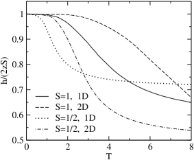
Figure 1: Boundary $h_{0}(T)$ in the $h-T$ plane separating region I, $h<h_{0}(T)$, where the equality $\omega_{\bm{q}}^{+-}=h$ [cf. Eq. (14)] may be fulfilled, from region II, $h>h_{0}(T)$, where $h>\omega_{\bm{q}}^{+-}$ for all $\bm{q}$.

Let us finally make some comments on the evaluation of the theory for different spin values.
(i) $S=\frac{1}{2}$: Using the identities $(S_{i}^{z})^{2}=1/4$ and $S_{i}^{z}S_{i}^{-}=-\frac{1}{2}S_{i}^{-}$ (cf. Eq. (22)) the sum rules (19) and (21) for $n=0$ simplify, where the higher sum rule (21) reduces to

$$z\left(\frac{1}{2}\langle S^{z}\rangle-C_{10}\right)=-\frac{1}{N}\sum_{\bm{q},i}(-1)^{i}\omega_{\bm{q}i}^{+-}A_{\bm{q}i}^{(0)}n(\omega_{\bm{q}i}).$$ (36)

Note that this sum rule may be also obtained from the exact representation (23) of the internal energy which in the case $S=1/2$ becomes (cf. Ref. JIR04, )

$$u = -\frac{z}{8}-\frac{h}{2}$$ (37)

$$- \frac{1}{N}\sum_{\bm{q}}\int_{-\infty}^{+\infty}\frac{d\omega}{2\pi}(\varepsilon_{\bm{q}}+\omega)Im\langle\langle S_{\bm{q}}^{+};S_{-\bm{q}}^{-}\rangle\rangle_{\omega}n(\omega)\phantom{mml}$$

with $\varepsilon_{\bm{q}}=z(1-\gamma_{\bm{q}})/2+h$, if $\langle\langle S_{\bm{q}}^{+};S_{-\bm{q}}^{-}\rangle\rangle_{\omega}$ given by Eq. (12) for $n=0$ is inserted into Eq. (37). The spectra $\omega_{\bm{q}}^{+-}$ and $\omega_{\bm{q}}^{zz}$ are given by Eqs. (10), (11), (29), and (30) with $\lambda^{+-}=0$ and $\lambda^{zz}=0$. We have to solve a closed system of coupled self-consistency equations for the seven quantities $\langle S^{z}\rangle$, $C_{10}^{(0)\mu\nu}$, $\alpha_{1}^{\nu\mu}$, and $\Delta^{\nu\mu}$ (or $\alpha_{2}^{\nu\mu}$). Note that in previous approachesJIR04 ; APP07 the simplified choice $\alpha_{2}^{\nu\mu}=\alpha_{1}^{\nu\mu}$ is taken disregarding the equality (34) and not using either the condition (17) (Ref. JIR04, ) or the higher sum rule (36) (Ref. APP07, ).
(ii) $S\geqslant 1$: Let us specify the identities (20) and (22) which are used to reduce the sum rules (19) and (21) for $n=2S-1$, respectively, for $S=1$ and $S=3/2$. For $S=1$ we have $(S_{i}^{z})^{3}=S_{i}^{z}$ and $(S_{i}^{z})^{2}S_{i}^{-}=-S_{i}^{z}S_{i}^{-}$, and for $S=3/2$ we get $(S_{i}^{z})^{4}=\frac{5}{2}(S_{i}^{z})^{2}-\frac{9}{16}$ and $(S_{i}^{z})^{3}S_{i}^{-}=-\frac{3}{2}(S_{i}^{z})^{2}S_{i}^{-}+\frac{1}{4}S_{i}^{z}S_{i}^{-}+\frac{3}{8}S_{i}^{-}$. For $S=1$ a closed system of coupled self-consistency equations for the ten quantities $\langle S^{z}\rangle$, $\langle(S^{z})^{2}\rangle$, $C_{10}^{(0)\mu\nu}$, $C_{10}^{(1)\mu\nu}$, $\alpha_{1}^{\nu\mu}$, and $\Delta^{\nu\mu}$ has to be solved.

In the case $h=0$ we have $\langle S^{z}\rangle=0$, and the correlators for $n=0$ only are needed. The spin-rotation symmetry, implying $C_{\bm{R}}^{(0)-+}=2C_{\bm{R}}^{(0)zz}=C_{\bm{R}}$, is preserved by the second-order theory with $\alpha_{1,2}^{+-}=\alpha_{1,2}^{zz}\equiv\alpha_{1,2}$ and $\lambda^{+-}=\lambda^{zz}\equiv\lambda$. Using $\langle(S^{z})^{2}\rangle=\frac{1}{3}S(S+1)$ following from Eq. (6), the Eqs. (10), (11), (29), and (30) yield the spectrum $\omega_{\bm{q}}^{+-}=\omega_{\bm{q}}^{zz}\equiv\omega_{\bm{q}}$ given by

$$\omega_{\bm{q}}^{2}=\frac{z}{2}(1-\gamma_{\bm{q}})\{\Delta+2z\alpha_{1}C_{10}(1-\gamma_{\bm{q}})\}$$ (38)

with

$$\Delta = \frac{4}{3}S(S+1)+2\{\lambda-(z+1)\alpha_{1}\}C_{10}$$ (39)

$$+ 2\alpha_{2}\{(z-2)C_{11}+C_{20}\},$$

which agrees with the result of Ref. SSI94, , if we put $\alpha_{2}=\alpha_{1}$.

The susceptibility $\chi_{S}=\chi_{0}^{zz}$ resulting from Eq. (34) is given by $\chi_{S}=2C_{10}/\Delta$. The correlators $C_{\bm{R}}^{(0)zz}$ are calculated from Eqs. (31) and (32) with $\langle S^{z}\rangle^{2}$ replaced by $\displaystyle{C^{zz}\equiv\frac{1}{N}\sum_{\bm{R}}C_{\bm{R}}^{(0)zz}}$ (see Refs. WI97, , ST91, ), where the condensation part $C^{zz}$ describes long-range order (LRO). At $T=0$ we have the exact result $C_{\bm{R}\neq 0}^{(0)zz}=\frac{1}{3}S^{2}$. The ferromagnetic LRO is reflected in the divergence of $\chi_{S}$, so that $\Delta(0)=\frac{4}{3}S(S+1)+\frac{4}{3}S^{2}\{\lambda-(z+1)\alpha_{1}+(z-1)\alpha_{2}\}=0$ and $\omega_{\bm{q}}=z\sqrt{2\alpha_{1}/3}S(1-\gamma_{\bm{q}})$. Then, by Eq. (31) we get $C_{\bm{R}}^{(0)zz}(0)=S/\sqrt{6\alpha_{1}}\delta_{\bm{R},0}+C^{zz}$ resulting in the sum rule [$\bm{R}=0$, cf. Eq. (6)] $\frac{1}{3}S(S+1)=S/\sqrt{6\alpha_{1}}+C^{zz}$, and in $C^{zz}=\frac{1}{3}S^{2}$ $(\bm{R}\neq 0)$. Finally, at $T=0$ we obtain $\alpha_{1}(0)=3/2$ and $\lambda(0)+(z-1)\alpha_{2}(0)=\frac{1}{2}(3z+1)-1/S$. For $S=1/2$ ($\lambda=0$) we have $\alpha_{2}(0)=\alpha_{1}(0)=3/2$. At finite temperatures there is no LRO in the 1D and 2D systems implying $C^{zz}=0$. The higher sum rule (21) for $n=0$ or, equivalently, Eq. (23) turns out to be trivially fulfilled. Therefore, following Ref. SSI94, , we put $\alpha_{2}=\alpha_{1}\equiv\alpha$ and $\lambda(T)=\lambda(0)=2-1/S$ and determine $\alpha(T)$ from the sum rule $C_{0}^{(0)zz}=\frac{1}{3}S(S+1)$.

III Quantum Monte Carlo simulations

In order to assess the accuracy of the approximations employed in the Green-function theory presented in the previous section we perform QMC simulations. The Heisenberg ferromagnets with $S=1/2$ and $S=1$ placed on chains or square lattices with periodic boundary conditions are simulated using the stochastic series expansion (SSE) method,sse1 ; sse2 which utilizes the high-temperature series expansion

$$Z={\rm Tr}\,e^{-\beta H}=\sum_{\alpha}\sum_{n=0}^{\infty}\frac{\beta^{n}}{n!}\left<\alpha\right|(-H)^{n}\left|\alpha\right>,$$ (40)

where the first sum is over a complete set of states $\left|\alpha\right>$, usually taken as the eigenvectors of the $S_{i}^{z}$ operator. By decomposing the Hamiltonian into diagonal and off-diagonal bond operators, introducing constant unit operators to assure positivity, and reexpanding (40), one finally ends up with a non-local loop representation which allows very efficient sampling.sse1 ; sse2 To minimize the effect of self-crossing and back-tracking, the directed loop-updating scheme is employed.

After initial thermalization with about $10^{6}$ Monte Carlo steps, the measurements are made after each step. During the simulation, the energy, magnetization, and correlation functions are measured and stored in a time series file, from which the specific heat and magnetic susceptibility can be computed using the fluctuation-dissipation relation. The correlation lengths are extracted from the exponential falloff of the correlation functions and for comparison also by means of the second-moment method.janke-greifswald06 Only for correlations smaller than one lattice spacing, small systematic deviations are visible. All those observables can be easily expressed by states of the spins on the lattice and the number and types of operators.sse3 The whole simulation usually takes of the order of $10^{7}$ Monte Carlo steps. The statistical error bars are estimated by the Jackknife method.Efron

The results presented in this paper are generated for $S=1/2$ chains of length up to $L=1024$ and for $S=1$ up to $L=64$. In two dimensions we simulate square lattices of edge length up to $L=64$. By comparing the results for different lattice sizes we made sure that for the investigated range of temperatures and fields, the thermodynamic limit of the considered observables lies within the statistical error bars of the numerical results.

IV RESULTS

As described in Sec. II, the quantities of the Green-function theory determining the thermodynamic properties have to be calculated numerically as solutions of a coupled system of non-linear algebraic self-consistency equations. To this end, we use Broyden’s methodnumrec which yields the solutions with a relative error of about $10^{-7}$ on the average, where the numerical error increases with decreasing field and temperature. The momentum integrals occurring in the self-consistency equations are done by Gaussian integration. Considering the $S=1/2$ ferromagnet, in Refs. JIR04, and APP07, the thermodynamic quantities, except for the transverse and longitudinal correlation lengths, are calculated. Therefore, we present only some results for $S=1/2$ (see Figs. 3, 7, and 15) which visibly improve those of Ref. JIR04, .

IV.1 Magnetic susceptibility

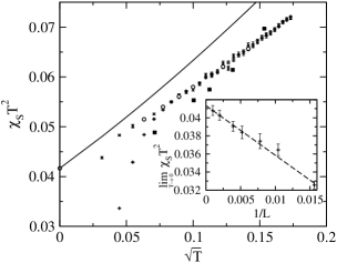
Figure 2: Zero-field susceptibility of the 1D $S=1/2$ ferromagnet. The results of the Green-function theory (solid line) and the QMC data ($+:L=256$, $\times:L=1024$) are compared with the QMC data of Ref. Kop89, ($\blacksquare$) and the Bethe-ansatz results of Ref. YT86, ($\circ$). In the inset the finite-size scaling of the zero-temperature limit of $\chi_{S}T^{2}$ calculated by QMC is depicted. The dashed line shows the least-square fit of the data by a linear dependence.

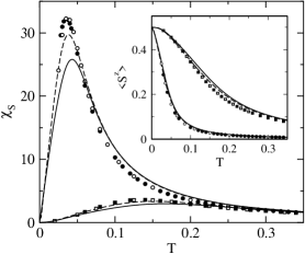
Figure 3: Susceptibility of the 1D $S=1/2$ ferromagnet at $h=0.005$ and 0.05, from top to bottom, where the results of the Green-function theory (solid lines) and of the Green-function method of Ref. APP07, (dashed lines), the QMC data (filled symbols, $L=128$), and the Bethe-ansatz results of Ref. JIR04, (open symbols) are shown. In the inset the 1D magnetization at $h=0.005$ and 0.05, from bottom to top, is depicted.

Let us first consider the susceptibility $\chi_{S}$ in the case $h=0$, $\chi_{S}=2C_{10}/\Delta$ ( see Sec. II). In one dimension, the low-temperature expansion yields $\displaystyle{\lim_{T\to 0}}\chi_{S}T^{2}=\frac{2}{3}S^{4}$ (Ref. SSI94, ). Note that this result agrees with that obtained by the modified spin-wave theory (MSWT).Tak86 For $S=1/2$ we have $\displaystyle{\lim_{T\to 0}}\chi_{S}T^{2}=0.041667$ which is in very good agreement with the Bethe-ansatz value $\displaystyle{\lim_{T\to 0}}\chi_{S}T^{2}=0.041675$ (Ref. YT86, ). On the other hand, previous QMC simulations by Handscomb’s method on an $N=256$ chain combined with a renormalization-group approachKop89 yield $\displaystyle{\lim_{T\to 0}}\chi_{S}T^{2}=0.0329$ (note that $\chi$ plotted in Ref. Kop89, and defined in Ref. KC89, is related to $\chi_{S}$ by $\chi=3\chi_{S}/S^{2}$). To resolve the discrepancy between the QMC results of Ref. Kop89, and the Bethe-ansatz value, we perform QMC simulations for chains up to $N=1024$ sites. The results at very low temperatures are shown in Fig. 2 (taking the same plot as in Ref. Kop89, ) and compared with the Bethe-ansatz data,YT86 the QMC data of Ref. Kop89, , and with the Green-function theory. Above a characteristic temperature, which decreases with increasing chain length, our QMC data agree very well with the Bethe-ansatz results. On the contrary, the QMC results of Ref. Kop89, for $\chi_{S}T^{2}$ are lower than ours by 4% on the average. To determine the limit $\displaystyle{\lim_{T\to 0}}\chi_{S}T^{2}$ from our QMC data, we perform a finite-size scaling analysis. To this end, for each chain length we linearly extrapolate the low-temperature linear part of the curve $\chi_{S}T^{2}$ to $T=0$ and fit the limiting values as function of $1/N$ by a linear dependence (see inset of Fig. 2). The extrapolation to $1/N=0$ yields $\displaystyle{\lim_{N\to\infty}\lim_{T\to 0}}\chi_{S}T^{2}=0.0413\pm 0.0005$ which agrees, within the given statistical error, with the Bethe-ansatz value.

The 2D zero-field susceptibility in the second-order Green-function theory increases exponentially for $T\to 0$, $\chi_{S}\propto\exp(2\pi S^{2}/T)$ (Ref. SSI94, ), where the exponent is smaller by a factor of two as compared with that found in the MSWTTak86 and in the renormalization-group approach.KC89

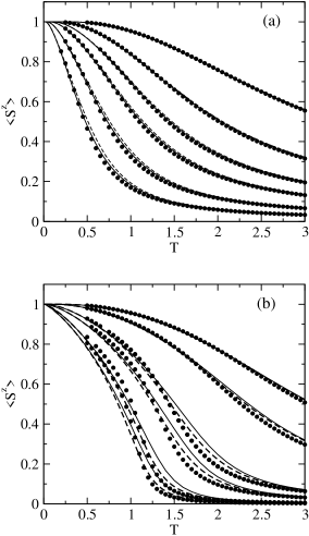
Figure 4: Magnetization of the (a) 1D and (b) 2D $S=1$ ferromagnet in magnetic fields of strengths (a) $h=0.1,0.2,0.4,0.6,1.0$, and 2.0, from bottom to top and (b) $h=0.005,0.01,0.05,0.1,0.5$, and 1.0, from bottom to top, as obtained by the Green-function theory (solid lines) and the QMC method for $L=64$ ($\bullet$), compared with RPA results (dashed lines).

Now we consider nonzero fields and calculate the susceptibility $\chi_{S}=\partial\langle S^{z}\rangle/\partial h$. First we show the magnetization. For $S=1/2$, as an example, $\langle S^{z}\rangle$ in the 1D model is depicted in the inset of Fig. 3. For the $S=1$ ferromagnet our analytical and QMC results in comparison with the RPA are plotted in Fig. 4. Let us emphasize the excellent agreement of the theory for the chain (Fig. 4(a)) with the QMC data over the whole temperature and field regions. For the 1D ferromagnet the RPA is a remarkably good approximation for $\langle S^{z}\rangle$, as was also found in the case $S=1/2$.JIR04 In two dimensions (Fig. 4(b)), as compared with the QMC data, the results of our theory at higher temperatures are somewhat worse than those of the RPA. This is in contrast to the 2D $S=1/2$ ferromagnet for which we obtain slightly better results than the RPA at all temperatures and fields (improving our previous findingsJIR04 ).

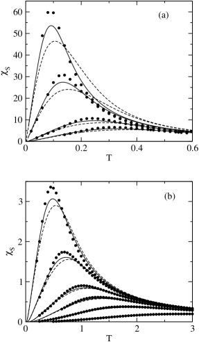
Figure 5: Susceptibility of the 1D $S=1$ ferromagnet (a) at low fields, $h=0.005,0.01,0.03$, and 0.05, from top to bottom, and (b) at higher fields, $h=0.1,0.2,0.4,0.6,1.0$, and 2.0, from top to bottom, where the Green-function (solid lines), the QMC ($\bullet$, $L=64$), and the RPA results (dashed lines) are shown.

The susceptibility for $h\neq 0$ vanishes at $T=0$. Therefore, $\chi_{S}(T)$ has a maximum at $T_{m}^{\chi}$, where $T_{m}^{\chi}$ increases and the height of the susceptibility maximum $\chi_{S}(T_{m}^{\chi})$ decreases with increasing field. For $S=1/2$, in Fig. 3 the low-field susceptibility in the 1D model is shown, where for $h=0.005$ a better agreement of the theory with the Bethe-ansatz results is found than in Ref. JIR04, . Note that our QMC data are in a very good agreement with the Bethe results. For comparison, in Fig. 3 the susceptibility in the simplified approach with $\alpha_{2}^{\nu\mu}=\alpha_{1}^{\nu\mu}$ (Ref. APP07, ), where the equality (34) is disregarded and the regularity condition (17) is used instead of the higher sum rule (36), is plotted as well. It is remarkable that $\chi_{S}$ in this approach is in a better agreement with the exact methods than the susceptibility in our extended theory with $\alpha_{2}^{\nu\mu}\neq\alpha_{1}^{\nu\mu}$. However, considering the correlation length the situation changes qualitatively (see below). For $S=1$ the susceptibility is plotted in Figs. 5 and 6. In one dimension (Fig. 5), the good agreement between Green-function theory and QMC corresponds to the results depicted in Fig. 4(a). As compared with the QMC data for the 2D model (Fig. 6), in RPA the maximum position $T_{m}^{\chi}$ is somewhat better reproduced than in our theory.

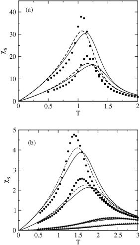
Figure 6: Susceptibility of the 2D $S=1$ ferromagnet (a) at very low fields, $h=0.005$ and 0.01, from top to bottom, and (b) at higher fields, $h=0.05,0.1,0.5$, and 1.0, from top to bottom, obtained by the Green-function theory (solid lines), QMC for $L=64$ (filled symbols), and RPA (dashed lines).

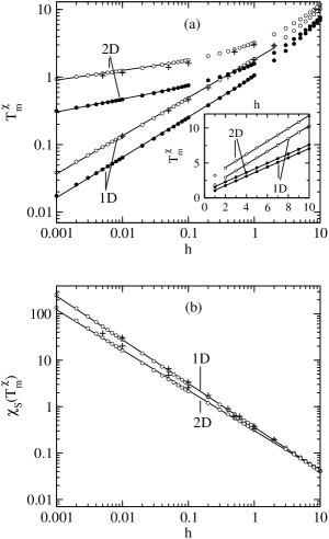
Figure 7: Field dependence of the (a) position and (b) height of the susceptibility maximum obtained by the Green-function theory for the $S=1/2$ ($\bullet$) and $S=1$ ($\circ$) ferromagnets and fit by power laws (solid lines) in comparison with the QMC data (+, $S=1$, $L=64$). The inset shows the fit of $T_{m}^{\chi}$ at high fields by a linear dependence. For clarity, $\chi_{S}(T_{m}^{\chi})$ is plotted for $S=1$ only.

To analyze the field dependence of $T_{m}^{\chi}$ and $\chi_{S}(T_{m}^{\chi})$ in more detail as in our previous paper,JIR04 the calculations are extended to a much broader field region, $0.001\leqslant h\leqslant 10$. As can be seen in Fig. 7(a), at low fields the theory may be well fitted by the power law

$$T_{m}^{\chi}=ah^{\gamma},$$ (41)

where the field regions and the values of $a$ and $\gamma$ are given in Table 1. Let us point out that the theory for the 1D $S=1/2$ model is in reasonable agreement with the Bethe-ansatz result at $h\leqslant 0.1$,JIR04 $a=0.765$ and $\gamma=0.576$. In the high-field region, $T_{m}^{\chi}$ obeys a linear dependence (cf. inset of Fig. 7(a)),

$$T_{m}^{\chi}=\tilde{a}h+\tilde{b}$$ (42)

with $\tilde{a}$ and $\tilde{b}$ given in Table 1. Note that the linear law (42) was not found in Ref. JIR04, . Our results for the maximum height $\chi_{S}(T_{m}^{\chi})$ as a function of $h$ may be well described in the whole field region $0.001\leqslant h\leqslant 10.0$ (see Fig. 7(b)) by the power law

$$\chi_{S}(T_{m}^{\chi})=bh^{\beta},$$ (43)

where the coefficients are given in Table 2. The values of $b$ and $\beta$ for $S=1/2$ slightly deviate (by about 5% on the average) from those found previously.JIR04 Again, our theory for $S=1/2$ is in reasonable agreement with the 1D Bethe-ansatz result at $h\leqslant 0.1$, $b=0.208$ and $\beta=-0.952$ (Ref. JIR04, ).

For comparison, we consider the power-law behavior in RPA. We find the RPA results in the low- and high-field regions to be well fitted by the laws (41)-(43), where the coefficients are in good agreement with the values given in Tables 1 and 2. More precisely, for the 1D and 2D $S=1/2$ and $S=1$ models the average deviations of the coefficients in the laws (41), (42), and (43) amount to about 6%, 3%, and 2%, respectively. For example, considering the $S=1/2$ ferromagnet in high fields, $2\leqslant h\leqslant 10$, we obtain the linear dependence (42) for the 1D (2D) case with $\tilde{a}=0.657$ (0.661) and $\tilde{b}=0.496$ (1.015) which yields a better fit than the power law (41). Recently, in Ref. HCP07, such a law was given for the 1D (2D) model in the region $3\;(4.4)\leqslant h\leqslant 6.5$. Even in this limited field region, we find the fit by the linear law (42) to be slightly better than the fit by the power law (41) (see Ref. HCP07, ).

Table 1: Validity regions ($h$) and coefficients of the power laws (41) and (42) for the susceptibility of the 1D and 2D $S=1/2$ and $S=1$ ferromagnets.

	$S=1/2$		$S=1$
	1D	2D	1D	2D
$h$	$0.001-1.0$	l $0.001-0.1$ l	l $0.001-2.0$ l	$0.001-0.1$
$a$	1.013	1.149	1.823	2.433
$\gamma$	0.596	0.192	0.565	0.144
$h$	$1.0-10.0$	$1.0-10.0$	$2.0-10.0$	$2.0-10.0$
$\tilde{a}$	0.661	0.666	0.917	0.929
$\tilde{b}$	0.443	0.961	1.136	2.494

Table 2: Coefficients of the power law (43) for the susceptibility of the 1D and 2D $S=1/2$ and $S=1$ ferromagnets in the field region $0.001\leqslant h\leqslant 10.0$

.

	$S=1/2$		$S=1$
	1D	2D	1D	2D
$b$	m 0.192 m	m 0.166 m	m 0.362 m	m 0.305 m
$\beta$	$-0.925$	$-0.850$	$-0.941$	$-0.867$

IV.2 Correlation length

To obtain the transverse and longitudinal correlation lengths $\xi^{+-}$ and $\xi^{zz}$ we consider the long-distance correlators $C_{\bm{R}}^{(0)-+}$ and $\bar{C}_{\bm{R}}^{(0)zz}\equiv C_{\bm{R}}^{(0)zz}-\langle S^{z}\rangle^{2}$ with $C_{\bm{R}}^{(0)zz}$ calculated by Eq. (31), respectively. Note that the temperature dependence of both $C_{\bm{R}}^{(0)-+}$ and $\bar{C}_{\bm{R}}^{(0)zz}$ exhibits a maximum, because the correlators vanish at $T=0$, following from Eqs. (31) and (35), and for $T\to\infty$. By the asymptotic ansatz

$$C_{\bm{R}}^{(0)-+}=A^{+-}\exp(-R/\xi^{+-}),$$ (44)

$$\bar{C}_{\bm{R}}^{(0)zz}=A^{zz}\exp(-R/\xi^{zz}),$$ (45)

and the logarithmic plot of the correlators as functions of $R=|\bm{R}|$ the inverse correlation lengths are evaluated numerically from linear fits.

In the literature, often the correlation length is determined from the expansion of the static spin susceptibility around the magnetic wavevector (see, e.g., Refs. ST91, , WI97, , and JIR05, ). In the ferromagnetic case we expand the static susceptibilities $\chi_{\bm{q}}^{+-}$ (resulting from Eqs. (10)-(12), (14), and (15)) and $\chi_{\bm{q}}^{zz}$ (given by Eqs. (27)-(29)) around $\bm{q}=0$, $\chi_{\bm{q}}^{\nu\mu}=\chi_{0}^{\nu\mu}/[1+(\xi_{\chi}^{\nu\mu})^{2}q^{2}]\;(\nu\mu=+-,\;zz)$. We obtain

$$\xi_{\chi}^{+-}=\sqrt{\alpha_{1}^{+-}\langle S^{z}\rangle/h}$$ (46)

and

$$\xi_{\chi}^{zz}=\sqrt{2\alpha_{1}^{zz}C_{10}^{(0)-+}/\Delta^{zz}}.$$ (47)

Deriving Eq. (46) the regularity condition (17) for $n=0$, which reads as $h\langle S^{z}\rangle=zC_{10}g_{0}$, and Eq. (16), yielding the relation $\Delta^{+-}=2h(C_{10}/\langle S^{z}\rangle-\alpha_{1}^{+-}\langle S^{z}\rangle)$, have been used. Let us point out that the correlation lengths $\xi_{\chi}^{\nu\mu}$ generally deviate from $\xi^{\nu\mu}$ defined by Eqs. (44) and (45).

First we consider the correlation length in zero field, where $\xi^{+-}=\xi^{zz}\equiv\xi$. In one dimension, the low-temperature expansion yields $\lim_{T\to 0}\xi T=S^{2}$ (Ref. SSI94, ) which agrees with the MSWT resultTak86 and, for $S=1/2$, with the result obtained by the thermal Bethe-ansatz method of Ref. Yam90, . The renormalization-group approach of Ref. Kop89, combined with QMC simulations yields $\lim_{T\to 0}\xi T=1.14S^{2}$. In Fig. 8 the zero-field correlation length of the 1D ferromagnet is shown. Let us stress the very good agreement of our QMC data for $S=1/2$ with the Bethe-ansatz results of Ref. Yam90, . Even on the finer scale of the inset, deviations are almost invisible. For comparison, also the QMC data of Ref. Kop89, and a one-parameter fit are given in the inset. Moreover, we obtain a good agreement of the Green-function theory, where $\xi$ is calculated from the definition (44), with our QMC data. In addition to $\xi$, in Fig. 8 the correlation length $\xi_{\chi}$ calculated for $S=1/2$ and $S=1$ by Eq. (47) [$\alpha_{1}^{zz}=\alpha$, $C_{10}^{(0)-+}=C_{10}$, $\Delta^{zz}=\Delta$ given by Eq. (39)] is plotted. For $T\lesssim 0.25$, i.e. $\xi>1$, $\xi_{\chi}$ nearly coincides with $\xi$. With increasing temperature, i.e., with decreasing $\xi<1$, the deviation of $\xi_{\chi}$ from $\xi$ appreciably increases. In the high-temperature limit we get $\xi_{\chi}^{-1}=\{3T/S(S+1)\}^{1/2}$ resulting from $C_{10}=2[S(S+1)]^{2}/9T$ (Ref. SSI94, ). In the following we plot $\xi_{\chi}$ in such cases only, where $\xi_{\chi}$ remarkably deviates from $\xi$.

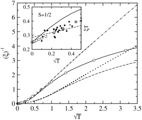
Figure 8: Zero-field correlation length of the 1D ferromagnet with $S=1/2$ obtained by the Green-function theory (solid lines) and by QMC simulations ($\times$, $L=32$) and with $S=1$ resulting from the theory (long-dashed line). For comparison, the correlation length $\xi_{\chi}$ determined from the expansion of the static susceptibility around $\bm{q}=0$ is plotted for $S=1/2$ (dotdashed line) and $S=1$ (dotted line). The results for $S=1/2$ are compared with the Bethe-ansatz data ($\circ$) of Ref. Yam90, and with the QMC data of Ref. Kop89, ($\bullet$) depicted in the inset together with a one-parameter fit (short-dashed line).

In two dimensions, the zero-field correlation length in the second-order Green-function theory increases exponentially for $T\to 0$, $\xi\propto\exp(\pi S^{2}/T)$ (Ref. SSI94, ). As is the case for the magnetic susceptibility, the exponent is smaller by a factor of two as compared with the MSWTTak86 and the renormalization-group approach.KC89

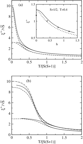
Figure 9: Transverse correlation length of the (a) 1D and (b) 2D ferromagnet with $S=1/2$ (solid lines) and $S=1$ (dashed lines) in the fields $h=0.01$ and 0.1, from top to bottom. In the 2D case at $h=0.01$, the correlation length $\xi_{\chi}^{+-}$ calculated from the static susceptibility is shown for $S=1/2$ (dotdashed line) and $S=1$ (dotted line). In the inset the results of the Green-function theory are compared with the Bethe-ansatz data of Ref. Tak91, ($\circ$) and the RPA (dotted line).

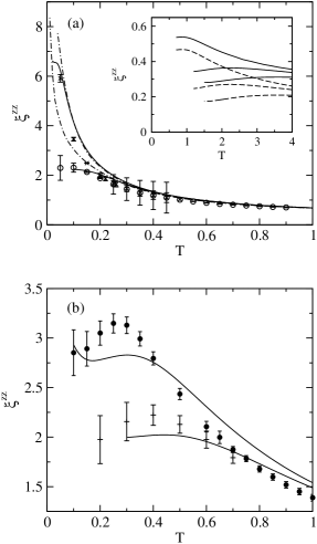
Figure 10: Longitudinal correlation length of the 1D ferromagnet with (a) $S=1/2$ and (b) $S=1$ in the fields (a) $h=0.005$ and 0.05 and (b) $h=0.05$ and 0.1, from top to bottom, calculated by the Green-function (solid lines) and QMC methods ($\times$, $\circ$; $L=32$ and $\bullet$, +; $L=32$) and, for $S=1/2$, by the method of Ref. APP07, (dotdashed lines). The inset exhibits the results for $S=1/2$ at the strong fields $h=1$, 3, and 5, from top to bottom, in comparison with the correlation length $\xi_{\chi}^{zz}$ (dashed lines) obtained from the static susceptibility.

For $h\neq 0$ the transverse and longitudinal correlation lengths reveal qualitatively different temperature dependences. Considering the transverse correlation length $\xi^{+-}$ shown in Fig. 9, the magnetic field cuts off the divergence of the zero-field correlation length at $T=0$ which corresponds to the absence of a phase transition and is evident from Eq. (46), $\xi_{\chi}^{+-}(T=0)=\sqrt{S/h}$ agreeing with the RPA result (52) derived in the Appendix. As can be seen in the inset of Fig. 9(a), in the 1D $S=1/2$ model we obtain a good agreement of our analytical results for $T=0.4$ and $h\leqslant 1.2$ with the Bethe-ansatz data of Ref. Tak91, . However, the comparison of the theory with the available Bethe data for $T=0.4$ and fields up to $h=4$ and for $T=0.2$ (Ref. Tak91, ) is hampered by numerical uncertainties resulting from too small values of $\Delta^{+-}$. Note the remarkably good agreement of $\xi^{+-}$ with the RPA results (see inset). Concerning the dimensional dependence, in contrast to the case $h=0$, $\xi^{+-}$ in one and two dimensions exhibits qualitatively the same behavior as $T\to 0$. In the 2D model [Fig. 9(b)], the deviation of $\xi_{\chi}^{+-}$ from $\xi^{+-}$ increases with decreasing temperature, i.e., with increasing $\xi^{+-}>1$ which is clearly seen at $h=0.01$ and is opposite to the behavior in the $h=0$ case.

In Fig. 10 the longitudinal correlation length of the 1D ferromagnet is shown, where the QMC data are found to be in a fair agreement with our theory. This refers, in particular, to the $S=1/2$ model, where our results obtained by the simplified approach of Ref. APP07, are plotted as well. Considering $h=0.05$, at low temperatures those results remarkably deviate from the QMC data and our extended theory with $\alpha_{2}^{\nu\mu}\neq\alpha_{1}^{\nu\mu}$. In contrast to $\xi^{+-}$, the behavior of $\xi^{zz}$ as $T\to 0$ is not conclusive which is due to numerical uncertainties at low temperatures, where the long-distance correlators $\bar{C}_{\bm{R}}^{(0)zz}$ needed to calculate $\xi^{zz}$ are very small. For example, for $S=1/2$ and strong fields [see inset of Fig. 10(a)] the relevant correlators in the temperature region, where results are not given, are smaller than about $10^{-10}$ to $10^{-14}$. Moreover, for $S=1$ the results of the theory are reliable only at $T>T_{0}\simeq 0.1$ and 0.3 for $h=0.05$ and 0.1, respectively [see Fig. 10(b)]. At $T<T_{0}$, the relevant correlators, being smaller than about $10^{-4}$, reveal an unreasonable behavior. This may be ascribed to our choice of a closed system of self-consistency equations for $S>1/2$, as described in Sec. II. Whereas the relative deviation of the NN correlators $C_{10}^{(0)zz}$ resulting from the self-consistency equations and from Eq. (31) is small (see Sec. II), the corresponding deviation of the correlators $\bar{C}_{10}^{(0)zz}$ becomes very large at low temperatures. Depending on the field and spin, the temperature dependence of $\xi^{zz}$ in the 1D ferromagnet reveals a maximum at $T_{m}^{\xi}>0$. This anomaly can be clearly seen in the 1D $S=1$ model at low fields [Fig. 10(b)]. On the other hand, in the 1D $S=1/2$ model the maximum appears at high fields, $h>0.8$ [see inset of Fig. 10(a)]. Moreover, as can be seen from Fig. 10, keeping the field $h=0.05$ fixed, the maximum develops with increasing spin. Note that a maximum of $\xi^{zz}$ at a finite temperature is not obtained by the approach of Ref. APP07, . To our knowledge, such an anomaly in the correlation length has not been found before. To get some insight into the maximum of $\xi^{zz}$, we first suggest that larger correlation lengths may be connected with larger correlation functions. Correspondingly, we consider the maximum of $\bar{C}_{\bm{R}}^{(0)zz}$ at $T_{m}^{zz}(R)$, where $T_{m}^{zz}(R)>T_{m}^{\xi}$. By a detailed analysis we find $T_{m}^{zz}(R)$ in the limit $R\to\infty$ to coincide with $T_{m}^{\xi}$ in all cases, where $\xi^{zz}$ has a maximum at $T_{m}^{\xi}>0$ (see Fig. 10), i.e., $\lim_{R\to\infty}T_{m}^{zz}(R)=T_{m}^{\xi}$. This result is corroborated by the conditions for a maximum which may be derived from the ansatz (45). We get $\frac{1}{R}\partial\ln\bar{C}_{\bm{R}}^{(0)zz}/\partial T=\frac{1}{R}\partial\ln A^{zz}/\partial T+\frac{1}{\xi}\partial\ln\xi/\partial T$. At $T_{m}^{zz}(R)$ we have $\frac{1}{\xi}\partial\ln\xi/\partial T=-\frac{1}{R}\partial\ln A^{zz}/\partial T$ and, for $R\to\infty$, $\partial\xi/\partial T=0$. As can be easily verified, the maximum condition $\partial^{2}\bar{C}_{\bm{R}}^{(0)zz}/\partial T^{2}<0$ results in $\partial^{2}\xi^{zz}/\partial T^{2}<0$. To compare the QMC and Green-function methods yielding the anomaly of $\xi^{zz}$ in the 1D $S=1$ model [Fig. 10(b)] in more detail, in Fig. 11 the distance dependence of the corresponding correlator $\bar{C}_{\bm{R}}^{(0)zz}$ at $h=0.05$ is depicted. For $T=0.5$ a very good agreement of both methods is found.

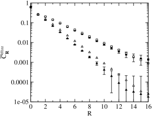
Figure 11: Correlation function $\bar{C}_{\bm{R}}^{(0)zz}=\langle S_{0}^{z}S_{\bm{R}}^{z}\rangle-\langle S^{z}\rangle^{2}$ vs $R=|\bm{R}|$ for the 1D $S=1$ ferromagnet in the field $h=0.05$ at $T=0.5$ and 1.0, from top to bottom, calculated by the Green-function theory (open symbols) and by QMC (filled symbols, $L=32$).

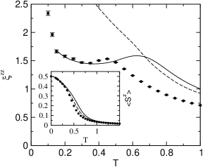
Figure 12: Longitudinal correlation length of the 2D $S=1/2$ ferromagnet at $h=0.05$ calculated by the Green-function theory (solid lines), QMC simulations ($\bullet$, $L=16$), and by the method of Ref. APP07, (dashed lines). In the inset the corresponding magnetization is plotted.

In two dimensions, the anomaly of $\xi^{zz}$ in the $S=1/2$ ferromagnet is more pronounced than in the 1D system and appears already at low fields, as can be seen in Fig. 12. In contrast to the 1D case, both the QMC data and the Green-function theory clearly reveal a minimum in addition to the maximum. Note that the statistical QMC errors in the interesting temperature region are smaller than the size of the symbols. Figure 12 demonstrates the qualitative effects of our extended theory ($\alpha_{2}^{\nu\mu}\neq\alpha_{1}^{\nu\mu}$) on the temperature dependence of $\xi^{zz}$ as compared with the simplified approach ($\alpha_{2}^{\nu\mu}=\alpha_{1}^{\nu\mu}$). Whereas this approach yields a slightly better agreement of the magnetization with the QMC data (see inset), it fails to describe the minimum-maximum anomaly.

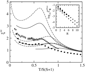
Figure 13: Longitudinal correlation length of the 2D ferromagnet with $S=1/2$ (solid lines) and $S=1$ (dashed lines) in the fields $h=0.01$, 0.05, and 0.10, from top to bottom, as compared with the QMC results at $h=0.05$ for $S=1/2$ ($\bullet$, $L=16$) and $S=1$ (+, $L=16$). The inset shows the correlation function $\bar{C}_{\bm{R}}^{(0)zz}=\langle S_{0}^{z}S_{\bm{R}}^{z}\rangle-\langle S^{z}\rangle^{2}$ vs $R=|\bm{R}|$ for the 2D $S=1/2$ ferromagnet in the field $h=0.05$ at $T=0.4$ and 0.6, from bottom to top, calculated by the Green-function theory (open symbols) and by QMC (filled symbols, $L=16$).

Figure 13 shows the field and spin dependence of the temperature behavior of $\xi^{zz}$ in the 2D ferromagnet. As results from the theory, the anomaly of $\xi^{zz}$ becomes more pronounced with decreasing field and with increasing spin. Let us point out that our QMC data for $h=0.05$ yield a minimum and a maximum of $\xi^{zz}$ for both the $S=1/2$ and $S=1$ models and give confidence in the results of the theory. As in the 1D model, the maximum of $\xi^{zz}$ at $T_{m}^{\xi}$ is related to the maximum of $\bar{C}_{\bm{R}}^{(0)zz}$ by $\lim_{R\to\infty}T_{m}^{zz}(R)=T_{m}^{\xi}$ in all cases shown in Fig. 13. The minimum of $\xi^{zz}$ results from the different temperature dependences of $\bar{C}_{\bm{R}}^{(0)zz}$ and $A^{zz}$ in the ansatz (45). In analogy to Fig. 11, for a more detailed comparison, the inset exhibits the correlator $\bar{C}_{\bm{R}}^{(0)zz}$ for $S=1/2$ and $h=0.05$ as function of the distance. The relative magnitude of the correlators at $T=0.4$ and 0.6 may be understood by the maximum in the temperature dependence of $\bar{C}_{\bm{R}}^{(0)zz}$.

IV.3 Specific heat

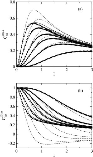
Figure 14: (a) Transverse and (b) longitudinal nearest-neighbor two-spin correlation functions of the 1D $S=1$ ferromagnet at the fields $h=0.1,0.2,0.4,0.6,1.0$, and 2.0, from left to right, obtained by the Green-function theory (solid lines), QMC ($\bullet$, $L=64$), and RPA (dashed lines).

Let us first consider the NN spin correlation functions $C_{10}^{(0)-+}$ and $C_{10}^{(0)zz}$ entering the internal energy $u=-\frac{z}{2}(C_{10}^{(0)-+}+C_{10}^{(0)zz})-h\langle S^{z}\rangle$. As an example, for the 1D $S=1$ model they are depicted in Fig. 14, where we obtain a very good agreement of the analytical results with the QMC data. On the contrary, the RPA results for $C_{10}^{(0)-+}$ remarkably exceed the QMC data, and for $C_{10}^{(0)zz}$ the RPA yields negative values being incompatible with the ferromagnetic SRO.

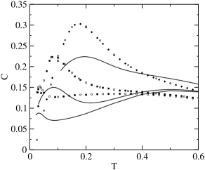
Figure 15: Specific heat of the 1D $S=1/2$ ferromagnet obtained by the Green-function (solid lines) and QMC (filled symbols, $L=128$) methods at low fields, $h=0.005,0.03$, and 0.1, from bottom to top, and compared with the Bethe-ansatz data of Ref. JIR04, (open symbols).

In Fig. 15 the specific heat $C=\partial u/\partial T$ for the 1D $S=1/2$ ferromagnet at low fields is plotted. Again, our QMC data agree very well with the Bethe-ansatz results.JIR04 At very low magnetic fields, the low-temperature maximum appearing, in the exact approaches at $h\lesssim 0.008$, in addition to the high-temperature maximum is much better described by the theory than we have found in Ref. JIR04, . In our Green-function theory this maximum appears up to higher fields, $h\leqslant 0.071$, and the deviation of the maximum position $T_{m,1}^{C}$ from the Bethe-ansatz and QMC values in the region $0.001\leqslant h\leqslant 0.01$ is less than 8%. Considering very low fields, $h=0.001$ to 0.01 in steps of 0.001, $T_{m,1}^{C}$ and the height $C(T_{m,1}^{C})$ are fit by the power laws

$$T_{m,1}^{C}=0.462\;h^{0.501},\;\;\;\;C(T_{m,1}^{C})=0.394\;h^{0.282}.$$ (48)

The exponents are in good agreement with the values of the Bethe-ansatz results,JIR04 $T_{m,1}^{C}=0.596\;h^{0.542}$ and $C(T_{m,1}^{C})=0.513\;h^{0.228}$. Note that the specific heat in the 2D model has only one maximum.JIR04

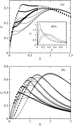
Figure 16: Specific heat of the 1D $S=1$ ferromagnet obtained by the Green-function theory (solid lines) (a) at low fields, $h=0.005,0.01,0.03$, and 0.05, from bottom to top, with the QMC results for $L=64$ (filled symbols) and (b) at higher fields, $h=0.1,0.2,0.4,0.6,1.0$, and 2.0, from left to right, in comparison with the QMC results for $L=64$ (filled symbols). The inset shows the RPA data at the fields given in (a), from top to bottom at $T=0.1$.

Figure 16 displays the specific heat of the 1D $S=1$ ferromagnet. At low magnetic fields, $0.007\lesssim h\lesssim 0.057$, besides the high-temperature maximum, a low-temperature maximum appears (see Fig. 16(a)). The position $T_{m,1}^{C}$ of this maximum obtained by the Green-function theory nearly agrees with the QMC results. As in the $S=1/2$ case,JIR04 in RPA a double maximum is not obtained (see inset of Fig. 16(a)), and the values of the specific heat maximum are much higher than the QMC values which is ascribed to a poor description of SRO in RPA (see also Fig. 14). The specific heat of the 1D $S=3/2$ ferromagnet is shown in Fig. 17. There is no low-temperature maximum, but only a hump at low enough fields. For higher spins qualitatively the same behavior is found. The specific heat for the 2D $S=1$ ferromagnet is plotted in Fig. 18. As in the case $S=1/2$,JIR04 in two dimensions only one maximum appears. At small fields the position of the maximum in the Green-function theory is remarkably shifted to higher temperatures as compared with the QMC data. Note that the RPA curves at low fields (see upper inset of Fig. 18) exhibit a too large maximum height, as was also found in the 1D model (inset of Fig. 16(a)).

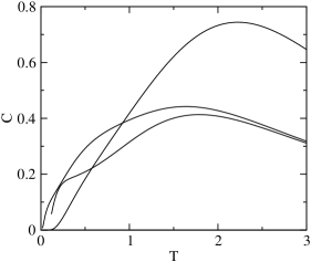
Figure 17: Specific heat of the 1D $S=3/2$ ferromagnet calculated by the Green-function theory at $h=0.01,0.1$ and 1.0, at $T=1.5$ from bottom to top.

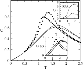
Figure 18: Specific heat of the 2D $S=1$ ferromagnet at $h=0.01$ and 0.05, from bottom to top, and, as depicted in the lower inset, at $h=0.1$ and 1.0, from left to right, where the Green-function (solid lines) and QMC (filled symbols, $L=64$) results are shown. In the upper inset the RPA results for $h=0.01$ and 0.05, from top to bottom, are plotted.

From our investigations of the maximum behavior of the specific heat in dependence on spin and dimension we conclude that the appearance of two maxima is a distinctive effect of quantum fluctuations which decrease with increasing spin and dimension. Note that in ferromagnets quantum fluctuations occur at nonzero temperatures only, whereas in antiferromagnets they are important already at $T=0$. The characterization of the occurrence of two maxima in the temperature dependence of the specific heat of the Heisenberg ferromagnet as a peculiar quantum effect is corroborated by recent QMC simulations of the 1D classical Heisenberg model and the 1D $S=1/2$ Ising model in a magnetic field,W06 where only one maximum in the specific heat was found.

IV.4 Comparison with experiments

Let us compare our results with experiments on $S=1/2$ quasi-1D ferromagnets, where we focus on the possible observation of two maxima in the temperature dependence of the specific heat as a characteristic feature of 1D ferromagnets in a magnetic field.

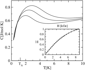
Figure 19: Specific heat of the copper salt TMCuC (Refs. LW79, and DRS82, , Néel temperature $T_{N}=1.24$K), as predicted by the theory for the $S=1/2$ 1D ferromagnet in the magnetic fields $H=2$kOe, 3kOe, and 4kOe, from bottom to top, with $J=6.18$ meV obtained from the fit of the reduced magnetization $\bar{m}=m(H)/m(H=8.7\text{kOe})$ at $T=4.1$K to experimental data ($\circ$) shown in the inset.

The copper salt TMCuC [(CH₃)₄NCuCl₃] was shownLW79 ; DRS82 to be a good 1D Heisenberg ferromagnet which is reflected in the small value of the Néel temperature $T_{N}=1.24$K for 3D ordering.DRS82 Determining the exchange energy $J$ by a least-squares fit of the theory for $S=1/2$ to the experimental data for the magnetization as a function of the magnetic field $H$ at $T=4.1$K,LW79 we obtain $J=6.18$meV and a very good agreement with experiments, as can be seen in the inset of Fig. 19. Note that the value of $J$ lies between the values given in Ref. LW79, ($J=5.17$meV) and in Ref. DRS82, ($J=7.76$meV). According to the QMC and Bethe-ansatz results for the 1D $S=1/2$ ferromagnet, two maxima of the specific heat occur for $h\lesssim 0.008$ or, using the relation $h=1.16\times 10^{-2}H$[kOe]$/J$[meV], for $H\leqslant 4$kOe. In Fig. 19 the specific heat, as predicted by the theory using the fit value of $J$, is plotted. The low-temperature maximum for $H=2$kOe, 3kOe, and 4kOe occurs at $T_{m,1}^{C}=2.0$K, 2.5K, and 2.9K, respectively. The high-temperature maximum (not shown in Fig. 19) appears at about $T_{m,2}^{C}=37.4$K with $C(T_{m,2}^{C})=1.18$J/molK for all fields considered. In the quasi-1D system the anomaly of the specific heat at $T_{N}$, which cannot be described by our theory for a purely 1D system, may mask the low-temperature maximum, if $T_{m,1}^{C}$ is not sufficiently larger than $T_{N}$. At $H=3$kOe (4kOe) we have $T_{m,1}^{C}/T_{N}=2.0$ (2.3). From this we predict that in TMCuC above $T_{N}$ two maxima in the specific heat at moderate magnetic fields, $H=3-4$kOe, may be observed.

Considering the quasi-1D organic ferromagnet p-NPNN (C₁₃H₁₆N₃O₄) in the $\gamma$ phase with $J=0.37$meV,TTN91 ; TKI92 where the phase transition at $T_{N}=0.65$K for $H=0$ persists up to $H=1.8$kOe ($T_{N}\simeq 0.5$K), two maxima of the specific heat above $T_{N}$ cannot be observed, because, at $h\lesssim 0.008$, ($H\lesssim 0.26$kOe), we have $T_{m,1}^{C}\lesssim 0.19\text{K}<T_{N}$. The analogous situation, in which the low-temperature maximum in the specific heat of the 1D ferromagnet cannot be seen, is found for the following compounds. Considering the ferromagnetic chains in the quasi-1D magnet $\beta$-BBDTA$\cdot$GaBr₄ with $J=0.375$meV,SGM06 we have $T_{m,1}^{C}\lesssim 0.19$K which is lower than the temperature of the specific-heat cusp, $T_{C}\geqslant 0.4$K, caused by the interchain coupling. For the CuCl₂-TMSO (tetramethylsulfoxide) [DMSO (dimethylsulfoxide)] salts with $J=3.36$ [3.88]meVSLW79 we get $T_{m,1}^{C}\lesssim 1.7$ [1.96]K being lower than the temperature of the susceptibility maximum, 3.9 [5.4]K, indicating the influence of the antiferromagnetic interchain coupling.

V SUMMARY

In this paper we have developed a second-order Green-function theory for the 1D and 2D Heisenberg ferromagnets in a magnetic field which extends our previous approachJIR04 to arbitrary spins and by the calculation of the correlation length. In addition, we have performed QMC simulations of the $S=1/2$ and $S=1$ models on a chain up to $N=1024$ sites and on a square lattice up to $N=64\times 64$ using the stochastic series expansion method with directed loop updates. The approximate analytical and quasi-exact numerical results turned out to be in good agreement, in particular for the ferromagnetic quantum spin chains. Analyzing the field dependence of the maximum in the temperature dependence of the magnetic susceptibility over a much broader field region as considered previouslyJIR04 we have found power laws for the position and height of the susceptibility maximum. The transverse and longitudinal correlation lengths were shown to have qualitatively different temperature dependences. Depending on spin, field, and dimension, the longitudinal correlation length $\xi^{zz}$ reveals an unexpected anomaly: with increasing temperature, $\xi^{zz}$ exhibits a minimum followed by a maximum. By a detailed investigation of the specific heat of the Heisenberg chain with arbitrary spin, two maxima in its temperature dependence at low magnetic fields were detected for $S=1/2$ and $S=1$, whereas for $S>1$ only one maximum appears, as in the 2D case. The existence of two specific-heat maxima was identified as a distinctive quantum effect. The theory was compared with magnetization experiments on the 1D copper salt TMCuC, and predictions for the temperature dependence of the specific heat, in particular for the occurrence of two maxima, were made which should be measurable experimentally.

AKNOWLEDGMENTS

The authors wish to thank J. Richter, N. M. Plakida and S. Wenzel for valuable discussions. This work was partially supported (L. B. and W. J.) by the EU through the Marie Curie Host Development Fellowship under Grant No. IHP-HPMD-CT-2001-00108 and the supercomputer time grant No. hlz12 of the John von Neumann Institute for Computing (NIC), Forschungszentrum Jülich. *

Appendix A RANDOM-PHASE APPROXIMATION

It is of interest to compare our results for finite magnetic fields with the RPA.Tjab67 Considering the equation of motion (2) the Tyablikov decoupling $i\dot{S_{\bm{q}}^{+}}=\omega_{\bm{q}}S_{\bm{q}}^{+}$ yields

$$\langle\langle S_{\bm{q}}^{+};S_{-\bm{q}}^{(n)-}\rangle\rangle_{\omega}=\frac{M^{(n)+-}}{\omega-\omega_{\bm{q}}},\;\;\;\;\omega_{\bm{q}}=z\langle S^{z}\rangle(1-\gamma_{\bm{q}})+h,$$ (49)

with $M^{(n)+-}$ given by Eq. (4). Comparing the correlation function $\langle(S_{i}^{z})^{n}S_{i}^{-}S_{i}^{+}\rangle$ resulting from Eq. (49) with the expression obtained by Eq. (6) multiplied by $(S_{i}^{z})^{n}$ and using the identity $\displaystyle{\prod_{m=-S}^{S}}(S_{i}^{z}-m)=0$, $\langle S^{z}\rangle$ is obtained asTjab67

$$\langle S^{z}\rangle = \{(S-P)(1+P)^{2S+1}+(1+S+P)P^{2S+1}\}\phantom{mn}$$ (50)

$$\times \{(1+P)^{2S+1}-P^{2S+1}\}^{-1},$$

where $P=(1/N)\sum_{\bm{q}}n(\omega_{\bm{q}})$. The transverse two-spin correlation functions $C_{\bm{R}}^{(0)-+}$ are calculated from Eq. (49) for $n=0$ which yields

$$C_{\bm{R}}^{(0)-+}=\frac{2\langle S^{z}\rangle}{N}\sum_{\bm{q}}n(\omega_{\bm{q}})\text{e}^{i\bm{qR}}.$$ (51)

The transverse correlation length $\xi^{+-}$ is calculated from the long-distance behavior of Eq. (51) according to Eq. (44). For comparison, the correlation length $\xi_{\chi}^{+-}$ may be obtained from the expansion of the static spin susceptibility $\chi_{\bm{q}}^{+-}$ around $\bm{q}=0$ (cf. Sec. IVB). We get

$$\xi_{\chi}^{+-}=\sqrt{\frac{\langle S^{z}\rangle}{h}}.$$ (52)

The longitudinal correlation functions $C_{\bm{R}\neq 0}^{(0)zz}$ cannot be obtained by the RPA, except for the NN correlation function $C_{10}^{(0)zz}$ which we evaluate proceeding as in Ref. JIR04, for $S=1/2$. That is, we calculate the internal energy in RPA starting from the exact representation (23) and inserting the RPA results (49) and (50), $C_{10}^{(1)-+}=(1/N)M^{(1)+-}\sum_{\bm{q}}n(\omega_{\bm{q}})\cos q_{x}$ with $M^{(1)+-}=3\langle(S^{z})^{2}\rangle-\langle S^{z}\rangle-S(S+1)$, and $\langle(S^{z})^{2}\rangle=S(S+1)-\langle S^{z}\rangle(1+2P)$ resulting from Eq. (6). Moreover, we perform the decoupling $C_{10}^{(1)zz}=\langle S^{z}\rangle\langle(S^{z})^{2}\rangle$. From $u,\;C_{10}^{(0)-+}$ and $\langle S^{z}\rangle$, the correlator $C_{10}^{(0)zz}$ may be calculated.

References

• (1) Quantum Magnetism, Lecture Notes in Physics, 645, edited by U. Schollwöck, J. Richter, D. J. J. Farnell, and R. F. Bishop (Springer, Berlin, 2004).
• (2) C. P. Landee and R. D. Willett, Phys. Rev. Lett. 43, 463 (1979).
• (3) C. Dupas, J. P. Renard, J. Seiden, and A. Cheikh-Rouhou, Phys. Rev. B 25, 3261 (1982).
• (4) M. Takahashi, P. Turek, Y. Nakazawa, M. Tamura, K. Nozawa, D. Shiomi, M. Ishikawa, and M. Kinoshita, Phys. Rev. Lett. 67, 746 (1991); Y. Nakazawa, M. Tamura, N. Shirakawa,
D. Shiomi, M. Takahashi, M. Kinoshita, and M. Ishikawa, Phys. Rev. B 46, 8906 (1992).
• (5) M. Takahashi, M. Kinoshita, and M. Ishikawa, J. Phys. Soc. Jpn. 61, 3745 (1992).
• (6) K. Shimizu, T. Gotohda, T. Matsushita, N. Wada, W. Fujita, K. Awaga, Y. Saiga, and D. S. Hirashima, Phys. Rev. B 74, 172413 (2006).
• (7) D. D. Swank, C. P. Landee, and R. D. Willett, Phys. Rev. B 20, 2154 (1979).
• (8) S. E. McLain, D. A. Tennant, J. F. C. Turner, T. Barnes, M. R. Dolgos, Th. Proffen, B. C. Sales, and R. I. Bewley, cond-mat/0509194.
• (9) W-H. Li, C. H. Perry, J. B. Sokoloff, V. Wagner, M. E. Chen, and G. Shirane, Phys. Rev. B 35, 1891 (1987); S. Feldkemper, W. Weber, J. Schulenburg, and J. Richter, ibid. 52, 313 (1995);
H. Manaka, T. Koide, T. Shidara, and I. Yamada, ibid. 68, 184412 (2003).
• (10) G. Kamieniarz and C. Vanderzande, Phys. Rev. B 35, R3341 (1987); G. M. Wysin and A. R. Bishop, ibid. 34, 3377 (1986).
• (11) P. Fröbrich, P. J. Jensen, and P. J. Kuntz, Eur. Phys. J. B 13, 477 (2000); P. Fröbrich, P. J. Jensen, P. J. Kuntz, and A. Ecker, ibid. 18, 579 (2000); P. Fröbrich and P. J. Kuntz, ibid. 32, 445 (2003).
• (12) P. Henelius, P. Fröbrich, P. J. Kuntz, C. Timm, and P. J. Jensen, Phys. Rev. B 66, 094407 (2002).
• (13) S. Schwieger, J. Kienert, and W. Nolting, Phys. Rev. B 71, 024428 (2005); M. G. Pini, P. Politi, and R. L. Stamps, ibid. 72, 014454 (2005).
• (14) R. Sellmann, H. Fritzsche, H. Maletta, V. Leiner, and R. Siebrecht, Phys. Rev. B 64, 054418 (2001); S. Pütter, H. F. Ding, Y. T. Millev, H. P. Oepen, and J. Kirschner, ibid. 64, 092409 (2001).
• (15) P. Fröbrich, P. J. Kuntz, and M. Saber, Ann. Phys. 11, 387 (2002).
• (16) S. V. Tyablikov, in Methods in the Quantum Theory of Magnetism (Plenum Press, New York, 1967).
• (17) I. Junger, D. Ihle, J. Richter, and A. Klümper, Phys. Rev. B 70, 104419 (2004).
• (18) T. N. Antsygina, M. I. Poltavskaya, I. I. Poltavsky, and K. A. Chishko, Phys. Rev. B 77, 024407 (2008).
• (19) F. Suzuki, N. Shibata, and C. Ishii, J. Phys. Soc. Jpn. 63, 1539 (1994).
• (20) I. Juhász Junger, D. Ihle, and J. Richter, Phys. Rev. B 72, 064454 (2005).
• (21) S. Winterfeldt and D. Ihle, Phys. Rev. B 56, 5535 (1997); 59, 6010 (1999).
• (22) J. Kondo and K. Yamaji, Prog. Theor. Phys. 47, 807 (1972); K. Yamaji and J. Kondo, Phys. Lett. 45 A, 317 (1973).
• (23) H. Shimahara and S. Takada, J. Phys. Soc. Jpn. 60, 2394 (1991); 61, 989 (1992).
• (24) D. Schmalfuß, J. Richter, and D. Ihle, Phys. Rev. B 70, 184412 (2004); 72, 224405 (2005).
• (25) P. J. Jensen and F. Aguilera-Granja, Phys. Lett. A 269, 158 (2000).
• (26) K. Elk and W. Gasser, in Die Methode der Greenschen Funktionen in der Festkörperphysik (Akademie-Verlag, Berlin, 1979); W. Nolting, in Quantentheorie des Magnetismus, vol. 2 (B. G. Teubner, Stuttgart, 1986).
• (27) A. W. Sandvik and J. Kurkijärvi, Phys. Rev. B 43, 5950 (1991).
• (28) O. F. Syljuasen and A. W. Sandvik, Phys. Rev. E 66, 046701 (2002).
• (29) W. Janke, in: Computational Many-Particle Physics, edited by H. Fehske, R. Schneider, and A. Weiße, Lect. Notes Phys. 739 (Springer, Berlin, 2008), pp. 79–140.
• (30) A. W. Sandvik, R. R. P. Singh, and D. K. Campbell, Phys. Rev. B 56, 14510 (1997).
• (31) B. Efron, The Jackknife, the Bootstrap and Other Resampling Plans (Society for Industrial and Applied Mathematics [SIAM], Philadelphia, 1982).
• (32) W. H. Press, S. A. Teukolsky, W. T. Vetterling and B. P. Flannery, in Numerical Recipes in Fortran 77: The Art of Scientific Computing (Cambridge University Press, Cambridge, 2001).
• (33) M. Takahashi, Prog. Theor. Phys. Suppl. 87, 233 (1986); Phys. Rev. Lett. 58, 168 (1987).
• (34) M. Yamada and M. Takahashi, J. Phys. Soc. Jpn. 55, 2024 (1986).
• (35) P. Kopietz, Phys. Rev. B 40, 5194 (1989).
• (36) P. Kopietz and S. Chakravarty, Phys. Rev. B 40, 4858 (1989).
• (37) A. Hu, Y. Chen, and L. Peng, Physica B 393, 368 (2007).
• (38) M. Yamada, J. Phys. Soc. Jpn. 59, 848 (1990).
• (39) M. Takahashi, Phys. Rev. B. 44, 12382 (1991).
• (40) S. Wenzel, private communication, 2006.