Bosonic reaction-diffusion processes on scale-free networks

Abstract

Reaction-diffusion processes can be adopted to model a large number of dynamics on complex networks, such as transport processes or epidemic outbreaks. In most cases, however, they have been studied from a fermionic perspective, in which each vertex can be occupied by at most one particle. While still useful, this approach suffers from some drawbacks, the most important probably being the difficulty to implement reactions involving more than two particles simultaneously. Here we introduce a general framework for the study of bosonic reaction-diffusion processes on complex networks, in which there is no restriction on the number of interacting particles that a vertex can host. We describe these processes theoretically by means of continuous time heterogeneous mean-field theory and divide them into two main classes: steady state and monotonously decaying processes. We analyze specific examples of both behaviors within the class of one-species process, comparing the results (whenever possible) with the corresponding fermionic counterparts. We find that the time evolution and critical properties of the particle density are independent of the fermionic or bosonic nature of the process, while differences exist in the functional form of the density of occupied vertices in a given degree class $k$. We implement a continuous time Monte Carlo algorithm, well suited for general bosonic simulations, which allow us to confirm the analytical predictions formulated within mean-field theory. Our results, both at the theoretical and numerical level, can be easily generalized to tackle more complex, multi-species, reaction-diffusion processes, and open a promising path for a general study and classification of this kind of dynamical systems on complex networks.

I Introduction

Many natural, social, and artificial systems exhibit heterogeneous patterns of connections and interactions that can be naturally described in terms of networks or graphs bollobas98 . Thus, complex network theory turns out to be the natural framework in which the functional and structural properties of complex systems belonging to completely different domains can be rationalized and investigated barabasi02 ; mendesbook ; newman-review ; caldarelli_book . This approach has recently proved to be very powerful, and systematic statistical analysis have allowed to recognize the existence of many characteristic features shared by a large class of different systems, the most peculiar being the small-world property watts98 and a large connectivity heterogeneity yielding a scale-free degree distribution barab99 . A graph is said to be small-world when the average topological distance between any pair of vertices is “small”, scaling logarithmically or slower with the system size $N$. On the other hand, defining the degree $k$ of a vertex as the number of connections linking it to other vertices, scale-free (SF) networks are characterized by a degree distribution $P(k)$ that decreases as a power-law,

$$P(k)\sim k^{-\gamma},$$ (1)

where $\gamma$ is a characteristic degree exponent, usually in the range $2<\gamma<3$.

The distinctive structural properties of networked systems, beyond being intrinsically interesting, have also a strong impact on the dynamical processes taking place on such systems dorogovtsev07:_critic_phenom , which can have practical implications in, e.g., understanding traffic behavior in technological systems such as the Internet romuvespibook . In particular, the heterogeneous connectivity pattern of SF networks with diverging second moment $\langle k^{2}\rangle$ (i.e., with $\gamma\leq 3$) can lead to very surprising dynamical properties, such as an extreme weakness in front of targeted attacks, aimed at destroying the most connected vertices havlin01 ; newman00 , as well as to the propagation of infective agents pv01a ; lloyd01 . After those initial discoveries, a large series of new results has been put forward and we refer the reader to Refs. bocaletti06:_compl_networ ; dorogovtsev07:_critic_phenom for recent reviews on the subject.

A powerful framework to describe many dynamical processes in a most general way is given by the theory of reaction-diffusion (RD) processes vankampen . RD processes are defined in terms of different kinds of particles or “species”, which diffuse stochastically (usually by performing a random walk) and interact among them according to a given set of reaction rules. Apart from their natural application to describe chemical reactions, RD processes are useful to represent any system in which different kinds of “agents” diffuse in space and dissappear, are created, or change their state, according to the state of other agents in a given neighborhood. An example of this kind of processes is the spread of diseases in population systems. An epidemic process leading to an endemic state can be described by the Susceptible-Infected-Susceptible (SIS) model epidemics , which corresponds to an RD process with two species (individuals), representing susceptible ($S$) and infected ($I$) individuals, which diffuse (with possible different diffusion rates) and interact through the reactions

$$\begin{array}[]{ccc}S+I&\to&2I,\\ I&\to&S,\end{array}$$ (2)

representing susceptible individuals becoming infected upon encountering an infected individual, and infected individuals spontaneously recovering.

RD processes on regular topologies (Euclidean lattices) have been extensively studied, and an elegant formalism has been developed to allow for a general description in terms of field theories RevModPhys.70.979 . On the other hand, the effects of more complex, heterogeneous, topologies have been taken into account only recently for simple processes originalA+A ; michelediffusion ; nohkim ; weber:046108 ; ke06:_migrat_driven ; chang07:_react_diffus_proces , and a systematic description of this interesting problem is still lacking. Moreover, so far most of the attention has been devoted to the restricted case of fermionic (or microscopic, in the chemistry jargon) RD processes, in which a vertex of the network cannot be occupied by more than one particle. In this context, numerical and analytical results have been put forward for the most simple RD processes, namely the diffusion-annihilation originalA+A ; michelediffusion and the diffusion-coagulation originalA+A ; weber:046108 processes. Although these results are undoubtedly interesting and offer an initial insight into the behavior of RD processes in heterogeneous networks, the adopted fermionic approach suffers from two considerable conceptual drawbacks: (i) there is no systematic framework for the description of this kind of processes, and both numerical models and theoretical approximations (through heterogeneous mean-field theory) must be considered on a case by cases basis; and (ii) it is relatively easy to deal with RD processes with at most order-two reactions (involving at most two particles), but it becomes more problematic to implement reactions among three or more particles. Thus, for example, a fermionic study of the three particles reaction $A+B+C\to\emptyset$ chang07:_react_diffus_proces requires the introduction of an artificial “intermediate” particle, created from the reaction of two particles, and that reacts itself with a third, leading to the actual annihilation event. In this sense, it seems more natural and realistic to consider instead bosonic (or mesoscopic) processes, in which there are no restrictions on the vertex occupancy, and for which, levering in what is already known for Euclidean lattices, it is possible to develop systematic analytical and numerical formalisms. Moreover, while some processes may naturally fit into a fermionic framework, other are intrinsically bosonic. For example, during the spreading of a disease (say HIV) on a social interaction network, each individual can only change its state (become infected) by contagion through one acquaintance in the network. However, the diffusion of a disease at the level of airport networks (for example, SARS) is better modeled by taking into account the number of infected individuals in each city colizza06:_predic . The bosonic version of RD processes on complex networks has been so far neglected, with the exception of Ref. v.07:_react , where it has been applied to the particular case of the SIS process, Eq. (2) (see also Ref. colizza07:_invas_thres for an extension of the model to weighted networks).

In this paper, we investigate the properties of general bosonic RD processes in complex heterogeneous networks, adopting a twofold continuous time approach based on heterogeneous mean-field (MF) theory and numerical simulations. We develop a general MF formalism, based on the standard law of mass action, that is able to describe any RD processes on general complex networks, taking a particularly simple form in one-species RD systems. For this case, general predictions, independent of the particular form of the reaction rules, can be made in the small particle density (diffusion-limited) regime. The formalism is applied and fully solved in two particular cases, the branching-annihilating random walk and the diffusion-annihilation problem, examples of RD systems with stationary states and monotonously decaying particle densities, respectively. In order to check the possible differences between the bosonic and fermionic implementations of the same problem, we consider at the same time both examples from the fermionic MF theory perspective. We find that both formalisms provide analogous results for the time evolution and critical properties of the dynamics. However, the two approaches are not completely equivalent: the functional form of the particle density restricted to vertices of given degree $k$ varies widely between the two approaches. Finally we check our results, and in particular the equivalence between fermionic and bosonic formalisms, by means of extensive computer simulations. Contrarily to previous approaches v.07:_react , in which a parallel updating scheme was defined for the particular model under scrutiny, we adopt a sequential continuous time algorithm that can be easily generalized for any RD process.

The paper is organized as follows. In Sec. II we define general bosonic RD processes in complex networks. Sec. III is devoted to the introduction of a generic analytical framework based on bosonic heterogeneous MF formalism, from which general predictions can be obtained for any kind of RD process. In Sec. IV we consider and solve some particular examples of RD processes, exhibiting steady states and a monotonously decaying density, namely the branching annihilating random walk and diffusion-annihilation processes, respectively. The predictions of heterogeneous MF theory are validated in Sec. V by means of numerical simulations. Finally, in Sec. VI we summarize and discuss our results.

II Bosonic RD processes in complex networks

We consider RD processes on complex networks, which are fully defined by the adjacency matrix $a_{ij}$, which takes the values $a_{ij}=1$ if vertices $i$ and $j$ are connected by an edge, and zero otherwise. From a statistical point of view, the network can also be described by its degree distribution $P(k)$ and its degree correlations, given by the conditional probability $P(k^{\prime}|k)$ that a vertex of degree $k$ is connected to a vertex of degree $k^{\prime}$ serrano07:_correl . Both descriptions are related through the formulas

$$P(k)=\frac{1}{N}\sum_{i}\delta(k,\sum_{j}a_{ij}),$$ (3)

where $\delta(x,y)$ is the Kronecker $\delta$ symbol, and michelediffusion

$$P(k^{\prime}|k)=\frac{1}{NkP(k)}\sum_{i\in k}\sum_{j\in k^{\prime}}a_{ij},$$ (4)

$N$ being the size of the network.

RD processes are defined as dynamical systems involving particles of $S$ different species $A_{\alpha}$, $\alpha=1,\ldots,S$, that diffuse stochastically on the vertices of the network and interact among them upon contact on the same vertex, following a predefined set of $R$ reaction rules. In a bosonic scheme, there is no limitation in the number of particles that a vertex can hold, therefore the occupation numbers $n^{\alpha}_{i}(t)$, denoting the number of particles of species $A_{\alpha}$ in vertex $i$ at time $t$, can take any value between $0$ and $\infty$. We will assume that diffusion in the network is homogeneous and takes place by means of random jumps between nearest neighbors vertices. Therefore, an $A_{\alpha}$ particle with a diffusion coefficient $D_{\alpha}$ at vertex $i$ will jump with a probability per unit time $D_{\alpha}/k_{i}$ to a vertex $j$ adjacent to $i$, where $k_{i}$ is the degree of the first vertex.

The reaction rules that particles experience upon contact, on the other hand, can be defined in the most general way by the corresponding stoichiometric equations guggenheim67:_therm

$$\sum_{\alpha=1}^{S}q_{\alpha}^{r}A_{\alpha}\stackrel{{\scriptstyle\lambda_{r}}}{{\longrightarrow}}\sum_{\alpha=1}^{S}(q_{\alpha}^{r}+p_{\alpha}^{r})A_{\alpha},\quad r=1,\ldots,R,$$ (5)

where $q_{\alpha}^{r}>0$ (we do not consider reactions involving the spontaneous creation of particles) and $p_{\alpha}^{r}\geq-q_{\alpha}^{r}$. The coefficients $q_{\alpha}^{r}$ and $p_{\alpha}^{r}$ define the $r$-th reaction process, while $\lambda_{r}$ is the probability per unit time that the reaction takes place. Given that the reactions take place inside the vertices, the only variation between a RD process in a complex network and a regular lattices lies in the diffusion step. As we will see, however, this variation alone can induce important differences between processes in these two reaction substrates.

III Heterogeneous continuous-time Bosonic mean-field formalism

A first analytical description of dynamical processes of complex networks can be obtained by means of heterogeneous MF theory dorogovtsev07:_critic_phenom . MF theory applied to networks is based in the assumption that all vertices with the same degree share essentially the same dynamic properties, and can therefore be consistently grouped into the same degree class. In the case of RD processes, and in order to allow for the possibility of network heterogeneity and large degree fluctuations, it becomes necessary to work with the density spectra $\rho_{\alpha,k}(t)$ pv01a ; pv01b , representing the partial density of $A_{\alpha}$ particles in vertices of degree $k$, and that is defined as

$$\rho_{\alpha,k}(t)=\frac{\bar{n}_{\alpha,k}(t)}{N_{k}},$$ (6)

where $\bar{n}_{\alpha,k}(t)$ is the average occupation number of particles $A_{\alpha}$ in the class of vertices of degree $k$ and $N_{k}=NP(k)$ is the number of vertices of degree $k$ in a network of size $N$. From the density spectra, the total density of $A_{\alpha}$ particles is given by

$$\rho_{\alpha}(t)=\sum_{k}P(k)\rho_{\alpha,k}(t).$$ (7)

Heterogeneous MF theory is given in terms of rate equations for the variation of the partial densities $\rho_{\alpha,k}(t)$, which in this case are composed by two terms: one dealing with the (linear) diffusion and another with the reactions, so we can write

$$\frac{\partial\rho_{\alpha,k}(t)}{\partial t}=\mathcal{D_{\alpha}}+\mathcal{R}_{\alpha}.$$ (8)

The diffusion term is easy to obtain by considering the diffusion dynamics at the vertex level. The total change of $A_{\alpha}$ particles at vertex $i$ is due to the outflow of particles jumping out at rate $D_{\alpha}$, plus the inflow corresponding to jumps of particles from nearest neighbors. Therefore, the diffusive component at the single vertex level satisfies the rate equation michelediffusion

$$\frac{\partial n_{\alpha,i}(t)}{\partial t}=-D_{\alpha}n_{\alpha,i}(t)+D_{\alpha}\sum_{j}\frac{a_{ij}}{k_{j}}n_{\alpha,j}(t).$$ (9)

Considering the density spectrum as the average

$$\rho_{\alpha,k}(t)=\frac{\sum_{i\in k}n_{\alpha,i}}{N_{k}}$$ (10)

and assuming that $n_{\alpha,i}(t)\simeq\bar{n}_{\alpha,k}(t)$, $\forall i\in k$, we obtain

$$\mathcal{D}_{\alpha}=-D_{\alpha}\rho_{\alpha,k}(t)+D_{\alpha}k\sum_{k^{\prime}}\frac{P(k^{\prime}|k)}{k^{\prime}}\rho_{\alpha,k^{\prime}}(t),$$ (11)

where we have used Eq. (4).

The reaction term can be directly derived from the law of mass action, according to which the rate of any (chemical) reaction is proportional to the product of the concentrations (or densities) of the reactants gardiner . Considering the set of all allowed processes Eq. (5), we obtain:

$$\mathcal{R}_{\alpha}=\sum_{r}p_{\alpha}^{r}\lambda_{r}\prod_{\beta}[\rho_{\beta,k}(t)]^{q_{\beta}^{r}}.$$ (12)

Collecting all terms, the rate equations for the density spectra can be written in the most general case as

$$\frac{\partial\rho_{\alpha,k}(t)}{\partial t} = -D_{\alpha}\rho_{\alpha,k}(t)+D_{\alpha}k\sum_{k^{\prime}}\frac{P(k^{\prime}|k)}{k^{\prime}}\rho_{\alpha,k^{\prime}}(t)$$ (13)

$$+ \sum_{r}p_{\alpha}^{r}\lambda_{r}\prod_{\beta}[\rho_{\beta,k}(t)]^{q_{\beta}^{r}},$$

while the total densities satisfy the equations

$$\frac{\partial\rho_{\alpha}(t)}{\partial t}=\sum_{r}p_{\alpha}^{r}\lambda_{r}\sum_{k}P(k)\prod_{\beta}[\rho_{\beta,k}(t)]^{q_{\beta}^{r}},$$ (14)

where we have used the degree detailed balance condition marian1

$$kP(k)P(k^{\prime}|k)=k^{\prime}P(k^{\prime})P(k|k^{\prime}).$$ (15)

It is noteworthy that Eq. (14) is explicitly independent of the particular form of the network’s degree correlations, which only appear implicitly through the form of the density spectra $\rho_{\alpha,k}$.

In the following, we will focus in the analysis of one-species RD processes, in which a single class of particles diffuse and react in the system, i.e. $S=1$. In this case, reactions of the same order can be grouped, and Eqs. (13) and (14) take the simpler forms, omitting the $\alpha$ index,

$$\frac{\partial\rho_{k}(t)}{\partial t} = k\sum_{k^{\prime}}\frac{P(k^{\prime}|k)}{k^{\prime}}\rho_{k^{\prime}}(t)+\sum_{q>0}\Gamma_{q}[\rho_{k}(t)]^{q},$$ (16)

$$\frac{\partial\rho(t)}{\partial t} = \rho(t)+\sum_{q>0}\Gamma_{q}\sum_{k}P(k)[\rho_{k}(t)]^{q},$$ (17)

where

$$\Gamma_{q}=-\delta(q,1)+\sum_{r}p^{r}\lambda_{r}\delta(q^{r},q),$$ (18)

and we have absorbed the diffusion rate $D$ into a redefinition of the time scale and the reaction rates $\lambda_{r}$.

RD processes with non diverging solutions for Eqs. (16) and (17) can be generally grouped in two classes: those yielding a particle density monotonously decaying in time and those exhibiting one or more steady states, with possibly associated phase transitions between different steady states. We will examine more closely these two cases in the following subsections. While a full theoretical analysis requires detailed information about the particular form of the reactions involved and the network’s degree correlations, it is possible, however, to make very general statements, and to obtain the asymptotic form of the solutions when the particle density $\rho$ is very small.

III.1 Steady-state Bosonic RD processes

RD processes with steady states possess nonzero solutions for the long time limit of Eq. (16). In particular, imposing $\partial_{t}\rho_{k}=0$, the steady states correspond to the solutions of the algebraic equation

$$\rho_{k}=-\frac{k}{\Gamma_{1}}\sum_{k^{\prime}}\frac{P(k^{\prime}|k)}{k^{\prime}}\rho_{k^{\prime}}(t)-\sum_{q>1}\frac{\Gamma_{q}}{\Gamma_{1}}[\rho_{k}]^{q},$$ (19)

where we assume $\Gamma_{1}\neq 0$. Since we do not consider the spontaneous creation of particles from void ($\Gamma_{0}=0$), $\rho_{k}=0$ is a solution of Eq. (19). This equation is extremely difficult to solve for a general correlation pattern $P(k^{\prime}|k)$, in order to find nonzero solutions. The condition for this nonzero solution to exist, however, can be obtained for any correlation pattern by performing a linear stability analysis marian1 in Eq. (16). Neglecting higher order terms, Eq. (16) becomes

$$\frac{\partial\rho_{k}(t)}{\partial t}\simeq\sum_{k^{\prime}}L_{kk^{\prime}}\rho_{k^{\prime}}(t),$$ (20)

where we have defined the Jacobian matrix

$$L_{kk^{\prime}}=\Gamma_{1}\delta(k^{\prime},k)+\frac{kP(k^{\prime}|k)}{k^{\prime}}.$$ (21)

It is easy to see that this matrix has a unique eigenvector $v_{k}=k$ and a unique eigenvalue $\Lambda=\Gamma_{1}+1$. Therefore, defining $\tilde{\Gamma}_{1}=\Gamma_{1}+1\equiv\sum_{r}p^{r}\lambda_{r}\delta(q^{r},1)$, a nonzero steady state is only possible when $\tilde{\Gamma}_{1}>0$, which translates in the presence of reaction processes with particle creation starting from a single particle. A phase transition from a zero density absorbing state marro99 can thus take place when $\tilde{\Gamma}_{1}$ changes sign. It is worth noting that the transition threshold takes the same form as in homogeneous MF theory, and it is thus independent of the network topology, contrary to what is found in the bosonic SIS model v.07:_react , and similar to the case of the fermionic contact process (CP) castellano06:_non_mean . This is due to the fact that SIS model is represented in terms of a two-species RD process, see Eq. (2), in which, moreover, a conservation rule (total number of particles) is imposed. This conservation rule, coupled to the diffusive nature of both species, is at the core of the zero threshold observed in the SIS on SF networks in the thermodynamic limit v.07:_react . The contact process, on the other hand, belongs (in Euclidean lattices) to the same universality class as the one-species Schlögl RD process janssen81:_noneq_phase , hence the topology-independent threshold in the fermionic CP in networks can be understood in view of the general result just derived in the bosonic framework.

To make further progress we restrict our attention to the case of uncorrelated networks, in which dorogorev

$$P(k^{\prime}|k)=\frac{k^{\prime}P(k^{\prime})}{\langle k\rangle}.$$ (22)

In this case, Eq. (19) can be rewritten as

$$\rho_{k}=-\frac{k\rho}{\langle k\rangle\Gamma_{1}}-\sum_{q>1}\frac{\Gamma_{q}}{\Gamma_{1}}[\rho_{k}]^{q},$$ (23)

Solving Eq. (23), we find an expression $\rho_{k}(\rho)$, depending implicitly on the particle density. Inserting this solution into Eq. (7), we obtain a self-consistent equation for $\rho$,

$$\rho=\sum_{k}P(k)\rho_{k}(\rho),$$ (24)

to be solved in order to obtain $\rho$ as a function of the RD parameters.

An approximate solution of Eq. (23) can be obtained in the limit of a very small particle density, that is, very close to the threshold. In this case, we can neglect the higher order terms in Eq. (23) and obtain

$$\rho_{k}\simeq-\frac{k}{\langle k\rangle\Gamma_{1}}\rho,$$ (25)

which makes only sense for $\Gamma_{1}<0$ (i.e. $0<\tilde{\Gamma}_{1}<1$, close to the phase transition). Inserting this expression into the self-consistent equation (24) yields no information. We must use, instead, the self-consistent relation coming from the steady-state condition of Eq. (17), namely

$$\rho=-\frac{1}{\tilde{\Gamma}_{1}}\sum_{q>1}\Gamma_{q}\sum_{k}P(k)[\rho_{k}]^{q}.$$ (26)

Inserting (25) into Eq. (26), and keeping only the term corresponding to the reactions of lowest order $q_{m}>1$, we obtain

$$\rho\simeq\left(\frac{(\langle k\rangle|\Gamma_{1}|)^{q_{m}}}{\langle k^{q_{m}}\rangle|\Gamma_{q_{m}}|}\right)^{1/(q_{m}-1)}\;{\tilde{\Gamma}_{1}}^{1/(q_{m}-1)},$$ (27)

where we have assumed $\Gamma_{q_{m}}<0$. This solution indicates that, in a finite size network and for sufficiently small densities, all bosonic RD systems with an absorbing state show a critical point ${\tilde{\Gamma}_{1}}^{c}=0$, with an associated density critical exponent $\beta=1/(q_{m}-1)$, coinciding again with the homogeneous MF solution. For SF networks with degree exponent $\gamma\leq q_{m}+1$, the particle density is additionally suppressed by a diverging factor $\langle k^{q_{m}}\rangle^{-1/(q_{m}-1)}$, signaling the presence of very strong size effects. For $\gamma>q_{m}+1$, the particle density is size independent, and we recover the standard MF solution for homogeneous systems.

III.2 Monotonously decaying Bosonic RD processes

As we have seen in Sec. III.1, a necessary condition for a RD system to have a decaying density is to have $\tilde{\Gamma}_{1}<0$. In this case, since no steady states are present, the full Eq. (16) must be solved. One can proceed by using a quasi-stationary approximation michelediffusion , assuming $\partial_{t}\rho_{k}(t)\ll\rho_{k}(t)$, which will be correct at low densities if $\rho_{k}(t)$ decays as a power law. Thus, neglecting the left-hand-side of Eq. (16), we obtain again Eq. (23). Solving it and inserting the corresponding expression of $\rho_{k}$ back into Eq. (17), we have an approximate equation for $\rho(t)$ that can give information about the long time behavior of the RD process.

This procedure can be simplified when considering the limit of very large time and very small particle density, where the concentration of particles is so low that the RD process is driven essentially by diffusion. In this diffusion-limited regime, it is possible to estimate the behavior of the particle density, which turns out to be independent of the correlation pattern of the network. Let us consider the limit case $\tilde{\Gamma}_{1}=0$, that is, in the absence of one particle reactions. Then, in the limit $\rho_{k}\to 0$, linear terms dominate in Eq. (16) and we can write

$$\frac{\partial\rho_{k}(t)}{\partial t}\simeq-\rho_{k}(t)+k\sum_{k^{\prime}}\frac{P(k^{\prime}|k)}{k^{\prime}}\rho_{k^{\prime}},$$ (28)

that is, the density behaves as in a pure diffusion problem. The situation is thus the following: the time scale for the diffusion of the particles is much smaller than the time scale for two consecutive reaction events, therefore at any time the partial density is well approximated by a pure diffusion of particles lovasz ; noh04:_random_walks_compl_networ ; rw_rings ,

$$\rho_{k}(t)\simeq\frac{k\rho(t)}{\langle k\rangle},$$ (29)

proportional to the degree $k$ and the total concentration of particles, and independent of degree correlations. Inserting this quasi-stationary approximation back into Eq. (17), we obtain

$$\frac{\partial\rho(t)}{\partial t}\simeq\sum_{q>1}\frac{\Gamma_{q}\langle k^{q}\rangle}{\langle k\rangle^{q}}\rho^{q}(t).$$ (30)

For small $\rho$, this equation is dominated by the reactions of smallest order $q_{m}$. Therefore, assuming $\Gamma_{q_{m}}<0$, we obtain the same decay in time as in the homogeneous MF theory,

$$\rho(t)\sim\left(\frac{(q_{m}-1)|\Gamma_{q_{m}}|\langle k^{q_{m}}\rangle}{\langle k\rangle^{q_{m}}}\right)^{-1/(q_{m}-1)}\;t^{-1/(q_{m}-1)},$$ (31)

again depressed by a size factor $\langle k^{q_{m}}\rangle^{-1/(q_{m}-1)}$ for $\gamma<q_{m}+1$, and completely independent of the correlation pattern.

If we were interested in the time behavior at intermediate densities, finally, the full Eq. (17) with the quasi-stationary approximation must be solved. This in general can only be done for uncorrelated networks.

IV Applications

In this Section we will apply the bosonic MF formalism developed above to the study of two examples of one-species RD processes, the branching-annihilating random walk and the diffusion-annihilation processes, representative of the classes of steady-state and monotonously decaying processes, respectively. For the sake of comparison, we will review also the predictions of corresponding fermionic MF theory, developed for an interacting particle system defined to simulate the process under scrutiny.

IV.1 Steady-state processes: Branching-annihilating random walks

On of the simplest RD processes leading to a nontrivial steady state is the generalized branching-annihilating random walk (BARW), defined by the reactions odor04:_univer

$$\begin{array}[]{ccc}qA&\stackrel{{\scriptstyle\lambda}}{{\longrightarrow}}&\emptyset\\ A&\stackrel{{\scriptstyle\mu}}{{\longrightarrow}}&(p+1)A\end{array},$$ (32)

that is, particles annihilate in $q$-tuples with a rate $\lambda$, and produce a number $p$ of offspring with rate $\mu$. Homogeneous MF theory predicts a continuous phase transition at $\mu_{c}=0$, with a particle density in the active phase

$$\rho\sim\mu^{1/(q-1)}.$$ (33)

For the particular case $q=2$, the transition belongs to different universality classes, according to the parity of the number of offsprings $p$ odor04:_univer . If $p$ is an odd number, it belongs to the universality class of directed percolation marro99 , the same as the CP. On the other hand, an even $p$, for which the parity of the number of particles in conserved, leads to a new, and different, universality class.

IV.1.1 Fermionic MF theory

When analyzing the process given by Eq. (32), the limitations of a fermionic approach become evident. Indeed, reactions involving more than two particles are difficult to describe in a fermionic framework, even from a conceptual point of view. In fermionic models originalA+A ; weber:046108 ; castellano06:_non_mean , usually diffusion and reactions are intimately linked, since particles jump between nearest neighbors and interact upon landing on an occupied vertex. Thus, when more than two particles are involved in a single reaction, complex schemes have to be devised to represent the process, schemes which, on the other hand, cannot be easily handled with standard sequential algorithms. Possible solutions could be the use of auxiliary “intermediate” particles chang07:_react_diffus_proces , or the design new algorithms that include the circumstance of different particles diffusing at the same time, but it is easy to figure out situations that would be potentially critical for such schemes (e.g. what happens in a pure diffusive process when one particle tries to move to an occupied vertex, while its starting point has been occupied by other particle?). On the other hand, it would be possible to construct such reaction schemes by involving a particle and two or more of its nearest neighbors, in a reaction step independent of diffusion. Such formalism, although possible in principle, would be nevertheless not general, since the number of reacting particles would be limited by the connectivity of the considered vertex, and it would also be more cumbersome to analyze from a MF perspective.

To allow for a consistent fermionic description, we will restrict our attention to the particular case $q=2$, in which only binary annihilation events are allowed, and that can be defined as a fermionic interacting particle system given by the rules:

• Each vertex can be occupied by at most one particle

• With probability $f$, a particle jumps to a randomly chosen nearest neighbor.

  • If the neighbor is empty, the particle fills it, leaving the first vertex empty.

  • If the neighbor is occupied, the two particles annihilate, leaving both vertices empty.

• With probability $1-f$, the particle generates $p$ offsprings. To do so:

  • $p$ different neighbors are randomly chosen

  • A new offspring is created on every selected vertex, provided this is empty (if it is already occupied, nothing happens).

In order to avoid problems with the offspring generation step, the minimum degree of the network is taken to be $m\geq p$. We note that this algorithm is not parity conserving, but we do not expect this to be relevant in networks at MF level.

With this implementation of the fermionic BARW in complex networks, we can see that the corresponding MF theory for the density spectrum takes the form

$$\frac{\partial\rho_{k}}{\partial t} = -f\rho_{k}-fk\rho_{k}\sum_{k^{\prime}}\frac{1}{k^{\prime}}P(k^{\prime}|k)\rho_{k^{\prime}}$$ (34)

$$+ fk(1-\rho_{k})\sum_{k^{\prime}}\frac{1}{k^{\prime}}P(k^{\prime}|k)\rho_{k^{\prime}}$$

$$+ (1-f)k(1-\rho_{k})\sum_{k^{\prime}}\frac{p}{k^{\prime}}P(k^{\prime}|k)\rho_{k^{\prime}},$$

where $p/k^{\prime}$ is the probability that one offspring of a particle in a vertex of degree $k^{\prime}$ arrives at a given nearest neighbor. For the particular case of uncorrelated networks, this equation simplifies to

$$\frac{\partial\rho_{k}}{\partial t}=-\rho_{k}-\frac{k\rho}{\langle k\rangle}\rho_{k}+(1-\rho_{k})(1+\nu)\frac{k\rho}{\langle k\rangle},$$ (35)

where we have rescaled the time and defined $\nu=(1-f)p/f$. The steady-state condition $\partial_{t}\rho_{k}=0$ yields the expression

$$\rho_{k}=\frac{k(1+\nu)\rho/\langle k\rangle}{1+k(2+\nu)\rho/\langle k\rangle}.$$ (36)

Application of the self-consistent condition $\rho=\sum_{k}P(k)\rho_{k}$ yields

$$\rho=\sum_{k}\frac{P(k)k(1+\nu)\rho/\langle k\rangle}{1+k(2+\nu)\rho/\langle k\rangle}\equiv\Psi(\rho).$$ (37)

The condition for the existence of a nonzero solution, $\Psi^{\prime}(0)\leq 1$, yields the threshold for the existence of a steady state

$$\nu>\nu_{c}=0\;\Rightarrow\;f<f_{c}=1.$$ (38)

In order to obtain the asymptotic behavior of $\rho$ as a function of $\nu$ in infinite SF networks, we proceed to integrate Eq. (37) in the continuous degree approximation, replacing sums by integrals and using the normalized degree distribution $P(k)=m^{\gamma-1}(\gamma-1)k^{-\gamma}$, where $m$ is the minimum degree in the network, to obtain

$$\rho=\frac{1+\nu}{2+\nu}F[1,\gamma-1,\gamma,-\frac{\langle k\rangle}{m(2+\nu)\rho}],$$ (39)

where $F[a,b,c,z]$ is the Gauss hypergeometric function abramovitz . Expanding the hypergeometric function in the limit of small $\rho$, close to the absorbing phase, we recover at lowest order for $\gamma>3$ the homogeneous MF result $\rho\sim\nu$. For $2<\gamma<3$, on the other hand, we obtain

$$\rho\sim\nu^{1/(\gamma-2)},$$ (40)

corresponding to an absorbing state transition, given by the control parameter $\nu$, with zero threshold and a critical exponent $\beta=1/(\gamma-2)$.

In any finite network this behavior is modified by finite size effects. To analyze it, we define $\Theta=\sum_{k}kP(k)\rho_{k}/\langle k\rangle$. The equation for the total density becomes then

$$\frac{\partial\rho}{\partial t}=\rho[\nu-(2+\nu)\Theta].$$ (41)

By imposing stationarity ($\partial_{t}\rho=0$) and non-zero solution ($\rho\neq 0$) one obtains

$$\Theta=\frac{\nu}{(2+\nu)}.$$ (42)

The expression of $\rho_{k}$, Eq. (36), can be simplified in the small density regime ($\rho\ll\langle k\rangle/[k(2+\nu)]$, $\forall k$) as

$$\rho_{k}\simeq\frac{k(1+\nu)\rho}{\langle k\rangle}.$$ (43)

By substituting this expression in the definition of $\Theta$ and inserting it into Eq. (42) one obtains

$$\rho=\frac{\langle k\rangle^{2}}{\langle k^{2}\rangle}\frac{\nu}{(1+\nu)(2+\nu)}.$$ (44)

SF networks of finite size have a cutoff or maximum degree $k_{c}(N)$ which is a function of Ndorogorev . Therefore, for uncorrelated SF networks with degree cutoff scaling with the network size as $k_{c}(N)\sim N^{1/2}$, finite size effects in the fermionic BARW lead to a size dependent density scaling as

$$\rho\sim N^{\frac{-(3-\gamma)}{2}}\nu.$$ (45)

IV.1.2 Bosonic MF theory

A bosonic formalism imposes no practical restriction to the maximum order that the reaction steps may have. Thus, the general BARW defined by the reactions Eq. (32) yields, within the bosonic MF formalism, to a rate equation Eq. (16) with $\tilde{\Gamma}_{1}=p\mu$ and $\Gamma_{q}=-q\lambda$, and $\Gamma_{q^{\prime}}=0$, for $q^{\prime}\neq\{1,q\}$, corresponding to an absorbing state phase transition at a critical particle creation rate $\mu_{c}=0$. The full analysis of this equation for any $q$ can be cumbersome, but we can immediately predict the behavior at large times in finite networks, which will be given by Eq. (27), namely

$$\rho \simeq \left(\frac{[\langle k\rangle p(1-p\mu)]^{q}}{\langle k^{q}\rangle q\lambda}\right)^{1/(q-1)}\;\mu^{1/(q-1)}$$ (46)

$$\sim N^{-\frac{q+1-\gamma}{2(q-1)}}\;\mu^{1/(q-1)},$$

for uncorrelated networks.

To proceed further, we consider the simplest case $q=2$, in which the density spectrum fulfills the equation

$$|\Gamma_{2}|\rho_{k}^{2}-\Gamma_{1}\rho_{k}-\frac{k\rho}{\langle k\rangle}=0,$$ (47)

yielding the solution

$$\rho_{k}=\frac{|\Gamma_{1}|}{2|\Gamma_{2}|}\left(-1+\sqrt{1+\frac{4|\Gamma_{2}|\rho k}{\langle k\rangle|\Gamma_{1}|^{2}}}\right),$$ (48)

where, in order to ensure the existence of the absorbing state, we must impose the condition $\Gamma_{1}<0$. In the large $k\rho$ regime, we observe here a distinctively square root dependence,

$$\rho_{k}\simeq\sqrt{\frac{k\rho}{|\Gamma_{2}|\langle k\rangle}},$$ (49)

different from the limiting constant behavior observed in the corresponding fermionic formulation, Eq. (36), as well as in other fermionic models pv01a ; michelediffusion ; castellano06:_non_mean . In the low density regime, on the other hand, we can Taylor expand Eq. (48) and recover, for the particular case of the BARW, the general relation Eq. (25). Thus, for particle densities smaller than the crossover density $\rho_{\times}$, with

$$\frac{4|\Gamma_{2}|\rho_{\times}k_{c}}{\langle k\rangle|\Gamma_{1}|^{2}}=1,$$ (50)

we recover, for uncorrelated SF networks, the asymptotic finite size solution for $q_{m}=2$, given by Eq. (46).

For networks in the infinite size limit, introducing the density spectrum of Eq. (48) into the self-consistent equation Eq. (24), we obtain

$$\rho=\sum_{k}P(k)\frac{|\Gamma_{1}|}{2|\Gamma_{2}|}\left(-1+\sqrt{1+\frac{4|\Gamma_{2}|\rho k}{\langle k\rangle(\Gamma_{1})^{2}}}\right).$$ (51)

In the continuous degree approximation, we have

$$\rho = \frac{|\Gamma_{1}|}{2|\Gamma_{2}|}\left(-1+\frac{2(\gamma-1)}{2\gamma-3}\sqrt{\frac{4|\Gamma_{2}|m\rho}{\langle k\rangle|\Gamma_{1}|^{2}}}\right.\times$$ (52)

$$\times \left.F[-\frac{1}{2},\gamma-\frac{3}{2},\gamma-\frac{1}{2},-\frac{\langle k\rangle|\Gamma_{1}|^{2}}{4|\Gamma_{2}|m\rho}]\right).$$

Expanding $F[a,b,c,z]$ in the limit of small $\rho$, we find

$$\rho \simeq \frac{\rho}{|\Gamma_{1}|}+\frac{|\Gamma_{1}|}{4|\Gamma_{2}|\sqrt{\pi}}\Gamma(2-\gamma)\Gamma(\gamma-3/2)\times$$ (53)

$$\times \left(\frac{4m|\Gamma_{2}|\rho}{\langle k\rangle(\Gamma_{1})^{2}}\right)^{\gamma-1}+\mathcal{O}(\rho^{2}).$$

At lowest order, and for $\gamma>3$, we recover the homogeneous MF solution $\rho\sim\tilde{\Gamma}_{1}\sim p\mu$. On the other hand, for $2<\gamma<3$, the nonzero solution of this equation is

$$\rho\sim\frac{\tilde{\Gamma}_{1}^{1/(\gamma-2)}}{|\Gamma_{2}|}\sim\frac{(p\mu)^{1/(\gamma-2)}}{\lambda},$$ (54)

corresponding to an absorbing state transition, given by the control parameter $\mu$, with zero threshold and a critical exponent $\beta=1/(\gamma-2)$, in full agreement with the results for the corresponding fermionic version of the model. We can use this last result to estimate the crossover density to the finite size solution Eq. (46). Inserting Eq. (54) into Eq. (50), and considering $\Gamma_{2}$ as a constant, we obtain that the finite size solution should be observed for a control parameter

$$\mu<\mu_{\times}=\frac{k_{c}^{2-\gamma}}{p}.$$ (55)

Therefore, for uncorrelated SF networks, finite size effects in the bosonic BARW should appear for a particle creation rate smaller that $\mu_{\times}\sim N^{-(\gamma-2)/2}$.

IV.2 Decay processes: Diffusion-annihilation process

The simplest case in the class of monotonously decaying RD processes corresponds to the general diffusion-annihilation process

$$qA\stackrel{{\scriptstyle\lambda}}{{\longrightarrow}}\emptyset,$$ (56)

which is the particular case of the BARW analyzed in Sec. IV.1 with $\mu=0$ (at the critical point). The homogeneous MF solution predicts a decay of the particle density

$$\rho(t)\sim t^{-1/(q-1)}.$$ (57)

In Euclidean lattices of dimension $d$, dynamical renormalization group arguments theoryA+A show that the behavior in Eq. (57) is correct for $d$ above the critical dimension $d_{c}=2/(q-1)$. Below it, we have instead $\rho(t)\sim t^{-d/2}$, with logarithmic corrections appearing at $d=d_{c}$.

IV.2.1 Fermionic MF Theory

As discussed in Sec. IV.1.1, in order to allow for a consistent fermionic description, we will restrict our attention to the binary diffusion-annihilation process with $q=2$, which can be implemented as a fermionic interacting system obeying the following rules originalA+A ; michelediffusion :

• Each vertex can be occupied by at most one particle

• Each particle jumps with probability $f$ to a randomly chosen nearest neighbor.

• If the neighbor is empty, the particle fills it, leaving the first vertex empty.

• If the neighbor is occupied, the two particles annihilate, leaving both vertices empty.

This model was analyzed in detail in Ref. michelediffusion . There it was observed that the rate equation for the density spectrum reads, in uncorrelated complex networks,

$$\frac{\partial\rho_{k}}{\partial t}=-\rho_{k}+\frac{k}{\langle k\rangle}(1-2\rho_{k})\rho,$$ (58)

where the probability $f$ has been absorbed into a rescaling of time. With a quasi-stationary approximation, the density spectrum at large times takes the form

$$\rho_{k}(t)=\frac{k\rho(t)/\langle k\rangle}{1+2k\rho(t)/\langle k\rangle},$$ (59)

which yields as a final equation for the density of particles

$$\frac{\partial\rho}{\partial t}=-2\frac{\rho^{2}(t)}{\langle k\rangle^{2}}\sum_{k}P(k)\frac{k^{2}}{1+2k\rho(t)/\langle k\rangle}.$$ (60)

In finite networks, for times larger that $t>t_{\times}$, with $k_{c}\rho(t_{\times})\simeq 1$, the denominator in Eq. (60) can be simplified to $1$, to obtain the limit behavior in finite size networks

$$\rho(t)\simeq\frac{\langle k\rangle^{2}}{2\langle k^{2}\rangle}\;t^{-1}.$$ (61)

In a network of infinite size, the full Eq. (60) must be integrated. Within the continuous degree approximation, this equation takes the form

$$\frac{\partial\rho}{\partial t}=-\rho(t)F[1,\gamma-2,\gamma-1,-\langle k\rangle/2m\rho(t)].$$ (62)

Expanding the Gauss hypergeometric function for small $\rho$, we obtain, for $\gamma>3$, the asymptotic long time behavior $\rho(t)\sim t^{-1}$ while for $2<\gamma<3$, one has

$$\rho(t)\sim t^{-1/(\gamma-2)}.$$ (63)

IV.2.2 Bosonic MF Theory

The general diffusion-annihilation process defined by reaction Eq. (56) leads to the general rate equation Eq. (16), with parameters $\tilde{\Gamma_{1}}=0$, $\Gamma_{q}=-q\lambda$, and $\Gamma_{q^{\prime}}=0$, for $q^{\prime}\neq\{1,q\}$. In finite networks and for large times, the behavior of the particle density will be given by Eq. (31), i.e.

$$\rho(t) \simeq \left(\frac{(q-1)q\lambda\langle k^{q}\rangle}{\langle k\rangle^{q}}\right)^{-1/(q-1)}\;t^{-1/(q-1)},$$ (64)

$$\sim N^{-\frac{q+1-\gamma}{2(q-1)}}\;t^{-1/(q-1)},$$

the last expression holding for uncorrelated SF networks.

Let us focus again in the simplest case $q=2$. The rate equation for the total density in uncorrelated networks takes the form

$$\frac{\partial\rho(t)}{\partial t}=-|\Gamma_{2}|\sum_{k}P(k)\rho_{k}^{2}(t).$$ (65)

Applying the quasi-stationary approximation for the density spectrum, we are led to the second order equation

$$|\Gamma_{2}|\rho_{k}^{2}+\rho_{k}-\frac{k}{\langle k\rangle}\rho=0,$$ (66)

whose only positive solution is

$$\rho_{k}=\frac{1}{2|\Gamma_{2}|}\left(-1+\sqrt{1+\frac{4|\Gamma_{2}|k}{\langle k\rangle}\rho}\right).$$ (67)

For a finite network with degree cut-off $k_{c}$, when the density is smaller that

$$\rho_{\times}=\frac{\langle k\rangle}{4|\Gamma_{2}|}k_{c}^{-1},$$ (68)

we can Taylor expand Eq. (67) to obtain the expression $\rho_{k}\simeq k\rho/\langle k\rangle$ and the asymptotic behavior given by Eq. (64). On the other hand, for large $k$ and $\rho$, we obtain

$$\rho_{k}\simeq\sqrt{\frac{k\rho}{4|\Gamma_{2}|\langle k\rangle}},$$ (69)

and we find again the peculiar square root behavior of the density spectrum on $k$, distinctive from the fermionic prediction.

The general solution in the infinite network limit can be obtained in this case by substituting the quasi-stationary approximation (67) into Eq. (65), to obtain

$$\frac{\partial\rho}{\partial t}=-\frac{1}{|\Gamma_{2}|}(1+2|\Gamma_{2}|\rho)+|\Gamma_{2}|\sum_{k}P(k)\sqrt{1+\frac{4|\Gamma_{2}|k}{\langle k\rangle}\rho}.$$ (70)

In the continuous degree approximation, and for SF networks, we obtain in the infinite network size limit

$$\frac{\partial\rho}{\partial t} = -\rho-\frac{1}{2|\Gamma_{2}|}+\frac{\gamma-1}{|\Gamma_{2}|(2\gamma-3)}\sqrt{\frac{4|\Gamma_{2}|m\rho}{\langle k\rangle}}\times$$ (71)

$$\times F[-\frac{1}{2},\gamma-\frac{3}{2},\gamma-\frac{1}{2},-\frac{\langle k\rangle}{4|\Gamma_{2}|m\rho}].$$

Considering the limit of large times and small densities, we can expand the hypergeometric function abramovitz , to obtain

$$\frac{\partial\rho}{\partial t}\simeq\frac{\Gamma(2-\gamma)\Gamma(\gamma-3/2)}{4|\Gamma_{2}|\sqrt{\pi}}\left(\frac{4m|\Gamma_{2}|\rho}{\langle k\rangle}\right)^{\gamma-1}+\mathcal{O}(\rho^{2})$$ (72)

for $2<\gamma<3$, whose solution is

$$\rho(t)\sim|\Gamma_{2}|^{\gamma-2}t^{-1/(\gamma-2)}\sim\lambda^{\gamma-2}t^{-1/(\gamma-2)}$$ (73)

that is, a power law decay with an exponent $1/(\gamma-2)$, again in agreement with the fermionic implementation of the process. From this expression we can estimate the time at which the crossover density in Eq. (68) is reached in SF network, namely

$$t_{\times}\sim k_{c}^{\gamma-2}\sim N^{(\gamma-2)/2},$$ (74)

taking the same functional form as the crossover control parameter for BARW in Eq. (55).

V Numerical simulations

As we have seen in the previous Sections, heterogeneous MF theory applied to steady state and monotonously decaying bosonic RD processes can make general predictions for the asymptotic behavior at finite networks, as well as give specific solutions for the infinite network size limit. In particular, we have seen that bosonic formalisms provide exactly the same results as their fermionic counterpart (whenever the fermionic mapping is possible) regarding the evolution of the particle density, the only difference being the form of the density spectra as a function of the degree $k$. In order to check these conclusions, we have performed extensive numerical simulations of bosonic and fermionic versions of the processes considered. To generate the network substrate for the RD processes, we have adopted the uncorrelated configuration model (UCM) ucmmodel that has the double benefit of producing SF networks without degree correlations mariancutofss ; krzywickirandom and with a tunable degree exponent. When correlations were desired, the configuration model (CM) bekessi72 ; benderoriginal ; bollobas1980 ; molloy95 was used, with the additional constraint of lack of multiple connections and self-loops originnewman ; maslovcorr ; mariancutofss .

Numerical simulations of fermionic RD processes must be tailored on a case by case basis, depending on the specific interacting particle system chosen to represent it originalA+A ; michelediffusion ; weber:046108 . As a general rule, simulations are performed following a sequential Monte-Carlo scheme marro99 . At the beginning, $N\rho_{0}$ particles are randomly distributed on the network, respecting the fermionic constrain that at most one particle can be present on a single vertex, i.e. $\rho_{0}\leq 1$. Then, at time $t$, a particle is randomly selected, and it undergoes the corresponding stochastic dynamics. The system is then updated according to the actions performed by the selected particle, and finally time is increased as $t\to t+1/n(t)$, where $n(t)$ is the number of particles at the beginning of the simulation step. For bosonic processes, we have used a continuous time formalism, details of which are given in the following subsection.

V.1 Continuous time bosonic simulations

Previous approaches to the numerical simulation of bosonic RD processes on complex networks v.07:_react relied on a parallel updating rule in which reaction and diffusion steps alternate: after all vertices have been updated for reaction, particles diffuse. This approach, while feasible, must again be tailored in a case by case basis, and strongly depends on the specific reactions of the process under consideration. Moreover, it introduces a subtle but relevant problem as far as the density spectrum is concerned. Indeed, while preserving the average density, pure diffusion immediately sets up the characteristic linear behavior $\rho_{k}(t)\sim k$. Thus, the density spectrum may assume (very) different aspects if we look at it after the reaction step or after the diffusion one. In order to overcome these difficulties we have opted instead for a sequential algorithm, which not only is absolutely general, but is in addition closer to the spirit of the continuous time rate equations we have developed to describe heterogeneous MF theory. The algorithm implemented is based in the one proposed in Refs. park ; park2 for the case of regular lattices. For one-species RD processes, the algorithm is described as follows: In networks of size $N$, initial conditions for simulations are usually a number $\rho_{0}N$ of particles randomly distributed on the network vertices, with no limitation on the occupation number of single vertices. To perform the dynamics, we consider the microscopic configuration $\{\mathcal{C}\}$ of the bosonic system, which is specified by the occupation number $n_{i}$ at each vertex $i$. A standard master equation approach vankampen implies that, for RD processes described by Eq. (8), the average number of events in an infinitesimal time $dt$ is

$$E(dt,\{\mathcal{C}\})=dt\sum_{i,r}\left(q^{r}!\,\lambda_{r}+\frac{\delta(q^{r},1)}{\sum_{r^{\prime}}\delta(q^{r^{\prime}},1)}\right)\omega(n_{i},q^{r})$$ (75)

where

$$\omega(n_{i},q^{r})=\left(\begin{array}[]{c}n_{i}\\ q^{r}\end{array}\right)$$ (78)

is the number of non-ordered $q^{r}$tuples of particles at vertex $i$. Since the algorithm considers all reacting $q-$tuples as equivalent, it is convenient focusing on reaction orders $q$ rather than on specific reactions $r$. In general, a particular RD process defines a finite set $Q$ of allowed reaction orders $q$, that can be formally indicated as $Q=(\{q\}|\,\exists r:q^{r}=q)$. At each time step one has to: (i) select a vertex $i$ (ii) select the order $q$ of the candidate reaction (iii) determine which reaction $r$ occurs. In details:

(i)

A vertex $i$ is selected with probability $W_{i}/M$, where $W_{i}=\sum_{q\in Q}\omega(n_{i},q)$ and $M=\sum_{i}W_{i}$;

(ii)

A particular $q=q^{*}$ (with $q^{*}\in Q$) is selected with probability $\omega(n_{i},q^{*})/W_{i}$;

(iii)

A particular reaction $r$ of order $q^{r}=q^{*}$ occurs with probability $q^{r}!\,\lambda^{r}\,\Delta t$, where $\Delta t$ is a configuration-independent time constant. In case $q^{*}=1$, in addition to reaction processes, the particle has the diffusion option, which is chosen with probability $\Delta t$ (since we set the diffusion coefficient $D=1$).

Time is updated as $t\to t+\Delta t/M$. It is clear park that to have valid transition probabilities $\Delta t$ must be chosen so that the condition

$$\left(\delta(q,1)+q!\sum_{r:q^{r}=q}\,\lambda_{r}\right)\Delta t\leq 1$$ (79)

holds for all values of $q$. With this prescription an average of $E(\Delta t,\{\mathcal{C}\})$ events occur in a time interval $\Delta t$.

V.2 Branching-annihilating random walks

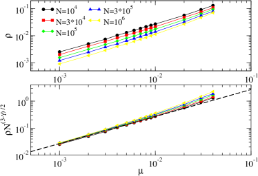
Figure 1: Average density of the bosonic BARW with $q=p=2$ at the steady state on uncorrelated UCM networks with $\gamma=2.5$. The annihilation rate is kept fixed at $\lambda=0.1$. Top: Density at the stationary state as a function of $\mu$, for different network sizes $N$. At any value of $\mu$, larger network sizes corresponds to smaller densities. Bottom: Check of the collapse predicted by Eq. (46). The dashed line has slope $1$.

In our numerical study of the BARW, we first focus in the behavior of the average particle density in the steady state as a function of the branching rate. As already observed in other dynamical systems in SF networks michelediffusion ; castellano07:_routes , we find it difficult to observe the infinite size limit behavior [Eq. (40) or (54)] in either bosonic of fermionic simulations, for the network sizes available within our computer resources. Therefore, we report the results for the finite size behavior, expected in finite networks, Eqs. (45) and (46). In Fig. 1 we plot the average density in the active phase of the bosonic BARW with $q=p=2$ as a function of the branching rate $\mu$. In the parameter range shown in this Figure (top panel), we observe that the density follows a linear behavior as a function of the branching parameter $\mu$. This linear dependence on $\mu$ corresponds to the asymptotic finite size solution predicted by Eq. (46), which is expected to hold in networks of finite size and for very small steady state densities. We can further check the accuracy of the prediction by noticing that, in SF uncorrelated networks, the prefactor in $\rho$ should scale with the system size as $\rho\sim\mu N^{-(3-\gamma)/2}$. Therefore, we should expect that a plot of $N^{(3-\gamma)/2}\rho$ as a function of $\mu$ would collapse for different network sizes. This is actually what we observe in Fig. 1 (bottom panel), where different curves are clearly laid one on top of the other for small values of $\mu$. As the density becomes larger, on the other hand, the collapse becomes less and less precise, in agreement with the fact that Eq. (46) is only valid in the very small density regime. Moreover, deviations from the collapse line set in earlier for large system sizes in agreement with Eq. (55), according to which finite size effects show up for values of $\mu$ smaller than $\mu_{\times}\sim N^{-(\gamma-2)/2}$.

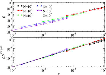
Figure 2: Average density of the fermionic BARW with $q=p=2$ at the steady state on uncorrelated UCM networks with $\gamma=2.5$. Top: Density at the stationary state as a function of the parameter $\nu$, for different network sizes $N$. Bottom: Check of the collapse predicted by Eq. (45). The dashed line has slope $1$.

In Fig. 2 we present analogous results for the fermionic version of the BARW. Here (top panel) we can observe a first difference with respect to the bosonic BARW: For small values of $N$, it is not possible to span a range of small values of $\nu$, due to the fact the the system falls quickly into the absorbing state. Small $\nu$ can only be explored using large $N$. The trend of all plots is, however, correct: Linear in $\nu$ and decreasing when increasing the network size. The data again collapses with the same functional form, now $\rho\sim\nu N^{-(3-\gamma)/2}$, for large systems sizes. The deviations at small $N$ and large $\nu$, however, seem now larger than in the bosonic case.

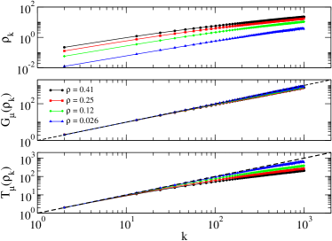
Figure 3: Density spectra in the bosonic BARW process with $q=p=2$ at the steady state on uncorrelated UCM networks with $\gamma=2.5$. Network size $N=10^{6}$. Top: Density spectra as a function of the degree $k$ for different steady state densities. Different stationary densities have been obtained fixing the annihilation parameter $\lambda=0.05$, and varying the branching parameter $\mu$. Center: Data collapse of the density spectra with different average stationary densities as predicted by Eq. (80). Bottom: Check of the Taylor expansion of the density spectra, as given by Eq. (81).

Having checked that the average density takes the same form in both bosonic and fermionic approaches, we focus now in the density spectra, in which differences between the two formalisms are predicted at the MF level. In the case of the bosonic BARW with $q=2$, the density spectra in the steady state, as given by Eq. (48), is characterized by a peculiar square root behavior. To check this form, we observe that, if we define the function

$$G_{\mu}(\rho_{k})\equiv\left[\left(\frac{4\lambda\rho_{k}}{1-2\mu}+1\right)^{2}-1\right]\frac{(1-2\mu)^{2}\langle k\rangle}{8\lambda\rho},$$ (80)

we expect $G_{\mu}(\rho_{k})=k$ for any values of the reaction parameters. In Fig. 3(center panel) we can see that this collapse works well for a wide range of $\rho$ values. Alternatively, we can consider the small density behavior, given by the general Eq. (25), which translates in the function

$$T_{\mu}(\rho_{k})\equiv(1-2\mu)\langle k\rangle\frac{\rho_{k}}{\rho}$$ (81)

being $T_{\mu}(\rho_{k})=k$. In Fig. 3(bottom panel) we observe a poor collapse of the curves, which is approximately attained only at very low densities, confirming the presence of strong nonlinearities at large $\rho$.

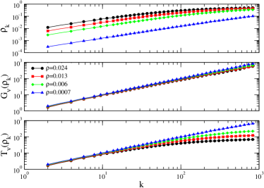
Figure 4: Density spectra for the fermionic BARW process with $q=p=2$ at the steady state on uncorrelated UCM networks with $\gamma=2.5$. Network size $N=10^{6}$. Top: Density spectra as a function of the degree $k$ for different steady state densities. Different stationary densities have been obtained varying the parameter $\nu$. Center: Data collapse of the density spectra for different steady state densities, as predicted by Eq. (82). Bottom: Check of the Taylor expansion of the density spectra, as given by Eq. (83).

In Fig. 4 we investigate the density spectrum of a fermionic BARW for different values of the total density. As we can observe (top panel), the spectra saturates to a constant value for large values of $\rho$ and $k$, as expected from the theoretical expression Eq. (36). On the other hand, this equation implies that the function

$$G_{\nu}(\rho_{k})\equiv\frac{\langle k\rangle\rho_{k}}{\rho(t)[(1+\nu)-(2+\nu)\rho_{k}]}$$ (82)

should satisfy $G_{\nu}(\rho_{k})=k$ for all $f$ and $p$. Considering the small density limit, on the other hand, a linear behavior of $\rho_{k}$ with $k$ is expected, translated again in the new function

$$T_{\nu}(\rho_{k})\equiv\frac{\langle k\rangle\rho_{k}}{\rho(t)(1+\nu)}$$ (83)

being $T_{\nu}(\rho_{k})=k$. While the collapse with the full shape of Eq. (36) (center panels in Fig. 4) is almost perfect, it is much worse if only the Tailor expansion in considered (bottom panel), being only approximately correct for very small densities.

V.3 Diffusion-annihilation process

To validate our theoretical approach for decaying RD systems, we have concentrated on the bosonic description of the processes, since the fermionic version described in Sec. IV.2.1 was already checked numerically in Ref. michelediffusion . We consider thus the general bosonic process $qA\to\emptyset$, at rate $\lambda$, for which a detailed analytical solution was given in Sec. IV.2.2. For the case $q=2$, again a peculiar square root behavior for the density spectrum was predicted in Eq. (67), which is corroborated in Fig. 5 by means of three different graphs. Again, from Eq. (67), defining the function

$$G_{0}(\rho_{k})\equiv\left((4\lambda\rho_{k}+1)^{2}-1\right)\frac{\langle k\rangle}{8\lambda\rho},$$ (84)

where $\lambda$ is the annihilation parameter, we will expect that $G_{0}(\rho_{k})=k$ for all times. In Fig. 5 (center panel) it is clear that the different curves, corresponding to different values of the average density $\rho(t)$, collapse well in agreement with the theoretical prediction. In the bottom panel, we check the general asymptotic expression for large times, Eq. (25). In this case, for small values of $8\lambda k\rho/\langle k\rangle$, we should expect the function

$$T_{0}(\rho_{k})\equiv\frac{k\rho(t)}{\langle k\rangle}$$ (85)

to be $T_{0}(\rho_{k})=k$, which holds when the times are large enough, but shows a clear bending at large degrees and large densities, signature again of the fact that it is fundamental to take into account the non-linearity of the spectrum.

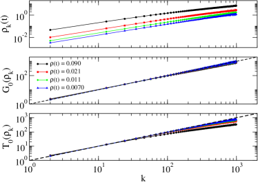
Figure 5: Density spectra of the bosonic RD process $2A\to\emptyset$ on uncorrelated UCM networks with $\gamma=2.5$. Network size $N=10^{6}$. Top: Density spectra as a function of the degree $k$ at different times (densities) from measures performed with fixed parameter $\lambda=0.1$. The curves show a bending in the large $k$ region for short times (large densities). Center: Data collapse of the density spectra at different times as predicted by Eq. (84). Bottom: Check of the Taylor expansion of the density spectra, as given by Eq. (85). The poor collapse at large $k$ confirms the presence of strong nonlinear terms at short times.

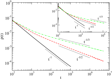
Figure 6: Density decay of the bosonic $qA\rightarrow\emptyset$ diffusion-annihilation processes in finite correlated and uncorrelated networks, for different values $q=2$ (full lines), $q=3$ (dashed lines) and $q=4$ (dot-dashed lines). For all values of $q$, the graphs show a tail of the form $t^{-1/(q-1)}$, as predicted in Eq. (64), both for uncorrelated (UCM) networks (main figure) and correlated (CM) networks (inset). Data obtained from networks of size $N=10^{5}$ with degree exponent $\gamma=2.5$. For all plots, the annihilation parameter was fixed at $\lambda=0.04$.

As in the case of the fermionic diffusion-annihilation process michelediffusion , it turns out that the asymptotic expression for infinite networks of the total particle density, Eq. (73), is very difficult to observe numerically, due to the very small range of the extension of the power-law behavior. We have therefore focused again on the general prediction for finite networks, Eq. (64), according to which the RD process $qA\to\emptyset$ shows a decay of the average density at large times of the form $\rho(t)\sim t^{-1/(q-1)}$, independently of the presence or absence of degree correlations. We present in Fig. 6 simulation results for three values of $q$, namely $q=2,3,4$, on uncorrelated networks SF generated with the UCM algorithm (main plot), and correlated SF networks generated with the CM prescription (inset). It is clear that the theoretical predictions are in perfect agreement with numerical data. This result is particularly relevant since, for $q>2$, it concerns purely bosonic processes, which do not have a fermionic counterpart.

The time independent prefactor of Eq. (64), moreover, states that the average density should be suppressed by the size term $(\langle k^{q}\rangle/\langle k\rangle)^{-1/(q-1)}$. More precisely, we can rewrite Eq. (57) as $\rho(t)\sim A(N,\gamma)^{-1/(q-1)}t^{-1/(q-1)}$, with

$$A(N,\gamma)\sim N^{(1+q-\gamma)/2}$$ (86)

in UCM networks, with cutoff $k_{c}(N)\sim N^{1/2}$. We have estimated the $A(N,\gamma)$ values by linear fits of the $\rho(t)^{-1}$ vs $t^{-1/(q-1)}$ curves for the $3A\rightarrow\emptyset$ process taking place on networks of different sizes (data not shown), and for two values of the degree exponent $\gamma$. We report the results in Fig. 7, where the scaling relation predicted by Eq. (86) is found to be in very good agreement with simulation data.

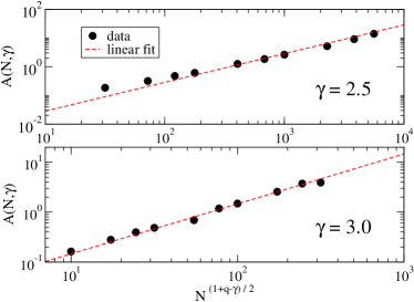
Figure 7: System size dependence of the density prefactor in the diffusion-annihilation process $3A\to\emptyset$. According to Eq. (86), we plot the prefactor $A(N,\gamma)$ as a function of $N^{(1+q-\gamma)/2}$. The good linear behavior confirms the predictions of bosonic heterogeneous MF theory in the diffusion-limited regime. Data obtained from networks with degree exponent $\gamma=2.5$. For all plots, the annihilation parameter was fixed at $\lambda=0.04$.

VI Discussion and conclusions

In this paper we have studied bosonic RD processes in SF networks introducing a general continuous-time framework which is well suited for both MF analytic calculations and computer simulations. At the MF level, we have developed the rate equations that characterize any generic RD process. We have considered in particular one-species RD processes, for which MF theory provides a natural way to classify all possible RD schemes. We have analyzed in detail both steady state and monotonously decaying processes from a general perspective, focusing also on specific examples, namely the BARW and diffusion-annihilation processes. For processes characterized by reactions not involving more than two particles, we have compared the results with a fermionic version of the same problems, implemented in terms of discrete interacting particle systems.

Beyond the obvious difference concerning the fact that the average density is bounded in fermionic processes while it is not in their bosonic version, both bosonic and fermionic MF formalisms render equivalent results for the density of particles in single-species RD processes, the main difference between both formalism lying in functional form of the density spectrum of particles. For high densities, the spectrum in bosonic systems goes in general as the power $k^{1/q_{M}}$, where $q_{M}$ is the highest order of the reactions defining the RD system, while for fermionic systems the behavior of the spectrum is in general algebraic. Thus, in the bosonic scheme, hubs become relatively less and less populated as more many-particle reactions are present, provided the average density is sufficiently high. In the very low density regime, on the other hand, the bosonic approach predicts spectra linear with $k$, a fact that allows to make general predictions for the behavior of any RD process in finite networks, which turns out to coincide with the homogeneous MF result, with a network size correction. This results confirms the relevance of finite size effects in dynamics on SF networks, already reported for fermionic systems michelediffusion ; castellano07:_routes , since the border between “high” and “low” densities is in general determined by the $\rho k_{c}(N)$ product.

Another interesting result concerns one-species bosonic RD processes with an absorbing state phase transition, where the critical point does not depend on the possible heterogeneity of the network, but is in general located at $\tilde{\Gamma}_{1}>0$. This condition translates in the presence of reaction processes with particle creation starting from a single particle and corresponds to the threshold independent of the network topology found in other fermionic systems castellano06:_non_mean . In order to observe effects of the connectivity heterogeneity in the threshold, more complex RD schemes, such as those involving two or more species, must be considered v.07:_react . On the other hand, the bosonic point of view allows to shed a different light on the value $\gamma=3$ usually associated to a frontier between regular ($\gamma>3$) and complex ($\gamma<3$) behavior for dynamical systems on SF networks. We can readily see that the value $\gamma=3$ emerges simply from considering dynamical processes involving at most two particle interactions. For general interactions involving $q$ particles, one will expect instead to obtain unusual results for $\gamma<q+1$ (see e.g. Eq. (46)).

The continuous time theoretical and numerical formalisms presented for bosonic processes have been developed in depth for the particular case of one-species processes, but they can be easily generalized to many species systems, opening thus the path to the study a large variety of processes of large relevance in the understanding of the topological effects of complex networks on dynamic and transport phenomena.

References

- (1) B. Bollobás, Modern Graph Theory (Springer-Verlag, New York, 1998).
- (2) R. Albert and A.-L. Barabási, Rev. Mod. Phys. 74, 47 (2002).
- (3) S. N. Dorogovtsev and J. F. F. Mendes, Evolution of networks: From biological nets to the Internet and WWW (Oxford University Press, Oxford, 2003).
- (4) M. E. J. Newman, SIAM Review 45, 167 (2003).
- (5) G. Caldarelli, Scale-Free Networks. Complex Webs in Nature and Technology (Oxford University Press, Oxford, 2007).
- (6) D. J. Watts and S. H. Strogatz, Nature 393, 440 (1998).
- (7) A.-L. Barabási and R. Albert, Science 286, 509 (1999).
- (8) S. Dorogovtsev, A. Goltsev, and J. Mendes, Critical phenomena in complex networks, 2007, e-print arXiv:0705.0010v2.
- (9) R. Pastor-Satorras and A. Vespignani, Evolution and structure of the Internet: A statistical physics approach (Cambridge University Press, Cambridge, 2004).
- (10) R. Cohen, K. Erez, D. ben Avraham, and S. Havlin, Phys. Rev. Lett. 86, 3682 (2001).
- (11) D. S. Callaway, M. E. J. Newman, S. H. Strogatz, and D. J. Watts, Phys. Rev. Lett. 85, 5468 (2000).
- (12) R. Pastor-Satorras and A. Vespignani, Phys. Rev. Lett. 86, 3200 (2001).
- (13) A. L. Lloyd and R. M. May, Science 292, 1316 (2001).
- (14) S. Bocaletti et al., Phys. Rep. 424, 175 (2006).
- (15) N. G. van Kampen, Stochastic processes in chemistry and physics (North Holland, Amsterdam, 1981).
- (16) O. Diekmann and J. Heesterbeek, Mathematical epidemiology of infectious diseases: model building, analysis and interpretation (John Wiley & Sons, New York, 2000).
- (17) D. C. Mattis and M. L. Glasser, Rev. Mod. Phys. 70, 979 (1998).
- (18) L. K. Gallos and P. Argyrakis, Phys. Rev. Lett. 92, 138301 (2004).
- (19) M. Catanzaro, M. Boguñá, and R. Pastor-Satorras, Phys. Rev. E 71, 056104 (2005).
- (20) J. D. Noh and S. W. Kim, Journal of the Korean Physical Society 48, S202 (2006).
- (21) S. Weber and M. Porto, Phys. Rev. E 74, 046108 (2006).
- (22) J. Ke et al., Phys. Rev. Lett. 97, 028301 (2006).
- (23) K. H. Chang et al., Journal of the Physical Society of Japan 76, 035001 (2007).
- (24) V. Colizza, A.Barrat, M. Barthelemy, and A. Vespignani, Proc. Natl. Acad. Sci. USA 103, 2015 (2006).
- (25) V. Colizza, R. Pastor-Satorras, and A. Vespignani, Nature Physics 3, 276 (2007).
- (26) V. Colizza and A. Vespignani, Phys. Rev. Lett. 99, 148701 (2007).
- (27) M. A. Serrano, M. Boguñá, R. Pastor-Satorras, and A. Vespignani, in Large scale structure and dynamics of complex networks: From information technology to finance and natural sciences, edited by G. Caldarelli and A. Vespignani (World Scientific, Singapore, 2007), pp. 35–66.
- (28) E. A. Guggenheim, Thermodynamics: An Advanced Treatment for Chemists and Physicists, 5th ed. (North Holland Physics Publishing, Amsterdam, 1967).
- (29) R. Pastor-Satorras and A. Vespignani, Phys. Rev. E 63, 066117 (2001).
- (30) C. W. Gardiner, Handbook of stochastic methods, 2nd ed. (Springer, Berlin, 1985).
- (31) M. Boguñá and R. Pastor-Satorras, Phys. Rev. E 66, 047104 (2002).
- (32) J. Marro and R. Dickman, Nonequilibrium phase transitions in lattice models (Cambridge University Press, Cambridge, 1999).
- (33) C. Castellano and R. Pastor-Satorras, Phys. Rev. Lett. 96, 038701 (2006).
- (34) H. K. Janssen, Z. Phys. B - Condensed Matter 42, 151 (1981).
- (35) S. N. Dorogovtsev and J. F. F. Mendes, Adv. Phys. 51, 1079 (2002).
- (36) L. Lovász, in Combinatorics, Paul Erdös is Eighty, edited by V. T. S. D. Miklós and T. Zsönyi (János Bolyai Mathematical Society, Bupadest, 1996), Vol. 2, pp. 353–398.
- (37) J. D. Noh and H. Rieger, Phys. Rev. Lett. 92, 118701 (2004).
- (38) A. Baronchelli and V. Loreto, Phys. Rev. E 73, 26103 (2006).
- (39) G. Ódor, Rev. Mod. Phys. 76, 663 (2004).
- (40) M. Abramowitz and I. A. Stegun, Handbook of mathematical functions. (Dover, New York, 1972).
- (41) B. P. Lee, J. Phys. A: Math. Gen. 27, 2633 (1994).
- (42) M. Catanzaro, M. Boguñá, and R. Pastor-Satorras, Phys. Rev. E 71, 027103 (2005).
- (43) M. Boguñá, R. Pastor-Satorras, and A. Vespignani, Euro. Phys. J. B 38, 205 (2004).
- (44) Z. Burda and Z. Krzywicki, Phys. Rev. E 67, 046118 (2003).
- (45) A. Bekessy, P. Bekessy, and J. Komlos, Stud. Sci. Math. Hungar. 7, 343 (1972).
- (46) E. A. Bender and E. R. Canfield, Journal of Combinatorial Theory A 24, 296 (1978).
- (47) B. Bollobás, Eur. J. Comb. 1, 311 (1980).
- (48) M. Molloy and B. Reed, Random Struct. Algorithms 6, 161 (1995).
- (49) J. Park and M. E. J. Newman, Phys. Rev. E 66, 026112 (2003).
- (50) S. Maslov, K. Sneppen, and A. Zaliznyak, Physica A 333, 529 (2004).
- (51) S.-C. Park, Phys. Rev. E 72, 036111 (2005).
- (52) S.-C. Park, Eur. Phys. J. B 50, 327 (2006).
- (53) C. Castellano and R. Pastor-Satorras, Routes to thermodynamic limit on scale-free networks, 2007, arXiv:0710.2784v1.