Constraint-preserving boundary treatment for a harmonic formulation of the Einstein equations

Abstract

We present a set of well-posed constraint-preserving boundary conditions for a first-order in time, second-order in space, harmonic formulation of the Einstein equations. The boundary conditions are tested using robust stability, linear and nonlinear waves, and are found to be both less reflective and constraint preserving than standard Sommerfeld-type boundary conditions.

1 Introduction

The numerical solution of the Einstein equations has, especially in the last two years, become a successful means of tackling many significant physical questions. The most topical of these questions concern the simulation of potential sources for gravitational-wave detection, and the propagation of gravitational waves. These problems are most commonly solved using finite-size computational domains, and this involves imposing a boundary condition on the physical system being simulated.

The standard treatment is to place a time-like boundary at a fixed coordinate location, and impose boundary conditions on the dynamical variables there. The particular conditions that are enforced ideally satisfy a number of properties. Most importantly, in order to ensure stability of the system, they should be compatible with the interior evolution equations so that the discretised system forms a well-posed initial-boundary-value problem (IBVP). Secondly, they should take into account the fact that Einstein evolutions always involve constraint equations as well as time evolution equations, and satisfy the constraints at all times. Otherwise, constraint violations introduced by the boundaries are likely to drive the evolution away from an Einstein solution. Finally, the boundary conditions should be compatible with physical considerations affecting the accuracy of the solution: they should be transparent to outgoing radiation, and restrict the amount of spurious incoming radiation from beyond the computational domain, which is assumed to contain all of the dynamics of interest.

To date, only the system of Friedrich-Nagy [1] satisfies the above conditions for the fully nonlinear vacuum Einstein equations. In this formulation the evolution equations are expressed first-order symmetric hyperbolic form and maximally dissipative boundary conditions guarantee well-posedness. There have been several attempts to approach the initial boundary value problem for the linearized Einstein equations. More recently, Kreiss and Winicour proposed well-posed, constraint-preserving boundary conditions for the linearized Einstein equations using the principle of frozen coefficients and pseudo-differential theory of systems for the first order system, which they then extrapolate to second-order [2]. Other approaches have been suggested by Rinne for non-reflecting boundary conditions which control incoming radiation by specifying data for the incoming fields of the Weyl tensor [3], and by Buchman and Sarbach, who have followed a similar route but specifying the incoming fields at the boundary [4].

The approach which we introduce in this paper is partially derived from a method first discussed in a series of related papers by Kreiss, Winicour and collaborators [2, 5, 6], combined with the SBP energy method discussed in Refs. [7, 8, 9]. By deriving energy estimates for the semi-discrete system using the “summation by parts” rule (defined below), one can ensure well-posedness [10, 11, 8, 12]. By applying this approach to boundary conditions which are radiation controlling and constraint-preserving, we are able to construct an IBVP which satisfies all of the above conditions in the linearized regime.

The conditions are derived for a harmonic formulation of the Einstein equations which has been implemented in [13, 14]. The evolution equations of the formulation, given explicitly in the next section, are first-order in time, second-order in space. We approximate these equations using standard finite-difference techniques, however to ensure a well-posed discrete IBVP, we have worked out finite-difference operators for this system which satisfy the summation by parts property. Since our computational domain uses Cartesian coordinates on a cube, we have had to develop consistent operators for the corners and edges, as well. Following the developments of [2, 15] and [16, 17], we are able to construct boundary conditions of a Sommerfeld type, which are both well-posed and satisfy both the Einstein and Harmonic constraints.

We have used the newly constructed boundary conditions in a number of practical tests and found them to perform extremely well in comparison with other standard techniques. Test evolutions include linear and nonlinear waves. In each case, the new boundary conditions are found to be more transparent to outgoing waves, as well as reducing the overall constraint violations on the grid. Further, the evolutions are stable against perturbations by high-frequency constraint violation (“noise”) added to the data, providing a strong demonstration of their robustness. Tests were also done for black hole space-times. For head-on collisions and inspiral, our boundary conditions showed improvements in reducing reflections and constraint preservation, and thus improved the waveform accuracy, but as the standard treatment was not long term stable for these tests due to instabilities at the excision boundary, we did not feel that it was appropriate to display in our results.

The plan of the paper is as follows: in the following section we introduce our harmonic evolution system, and describe the evolution variables, equations, and constraints. Section 2 describes the implementation of a harmonic evolution system for the Einstein equations. In particular, Section 2.2 describes the construction of finite-difference operators which ensure that the discretisation of our evolution equations remains well-posed, including the boundary faces, corners and edges. The boundary treatment is described in Section 3. In Section 3.2 we present the derivation of constraint preserving Sommerfeld type conditions for this system. Finally, in Section 4, we discuss a number of test cases to which these boundary conditions have been applied, and demonstrate their usefulness in ensuring stability and improving accuracy in a variety of scenarios.

2 The harmonic evolution system

2.1 Formulation of the evolution equations

The decomposition of the Einstein tensor into evolution equations and constraints leaves four degrees of freedom in the space-time metric that are not set by the field equations themselves, but can be freely specified. In a $3+1$ approach, these four degrees of freedom are determined by the choice of the lapse and shift, which amounts to specifying four out of ten metric components. The Arnowitt-Deser-Misner (“ADM”) equations [18] are a well known reduction of the Einstein system corresponding to this style of gauge choice.

An alternate approach to fixing the gauge degrees of freedom specifies the action of the wave operator on the coordinates, regarded as four scalar quantities. This is done by first choosing four functions $F^{\alpha}$ and then constructing a coordinate map $x^{\alpha}$ subject to the condition [19] that the d’Alembertian of each coordinate is

$$\Box x^{\alpha}=\frac{1}{\sqrt{-g}}\partial_{\mu}\left(\sqrt{-g}g^{\mu\beta}\partial_{\beta}x^{\alpha}\right)=F^{\alpha}\,,$$ (1)

rewriting Eqs. (1) as constrained variables

$$C^{\alpha}:=\Box x^{\alpha}-F^{\alpha}=0\,,$$ (2)

and using them in combination with the Einstein tensor $G^{\mu\nu}$ one obtains the generalized harmonic evolution system

$$E^{\mu\nu}:=G^{\mu\nu}-\nabla^{(\mu}C^{\nu)}+\frac{1}{2}g^{\mu\nu}\nabla_{\alpha}C^{\alpha}=0\,.$$ (3)

In terms of these variables, the vacuum Einstein equations are a system of ten wave equations acting on the metric components, coupled through the coefficients of the wave operator and the source terms.

Using the densitized inverse metric $\tilde{g}^{\mu\nu}:=\sqrt{-g}g^{\mu\nu}$ as evolution variables, the harmonic constraints (2) take the form

$$C^{\alpha}=-\frac{1}{\sqrt{-g}}\partial_{\beta}\tilde{g}^{\alpha\beta}-F^{\alpha}=0\,,$$ (4)

while for the evolution equations we obtain

$$\partial_{\rho}\left(g^{\rho\sigma}\partial_{\sigma}{\tilde{g}}^{\mu\nu}\right)-2\sqrt{-g}g^{\rho\sigma}g^{\tau\lambda}\Gamma^{\mu}_{\rho\tau}\Gamma^{\nu}_{\sigma\lambda}-\sqrt{-g}(\partial_{\rho}g^{\rho\sigma})(\partial_{\sigma}g^{\mu\nu})+\frac{g^{\rho\sigma}}{\sqrt{-g}}(\partial_{\rho}g^{\mu\nu})(\partial_{\sigma}g)$$

$$+\frac{1}{2}g^{\mu\nu}\bigg{(}\frac{g^{\rho\sigma}}{2g\sqrt{-g}}(\partial_{\rho}g)(\partial_{\sigma}g)+\sqrt{-g}\Gamma^{\tau}_{\rho\sigma}\partial_{\tau}g^{\rho\sigma}+\frac{1}{\sqrt{-g}}(\partial_{\sigma}g)\partial_{\rho}g^{\rho\sigma}\bigg{)}$$

$$+2\sqrt{-g}\nabla^{(\mu}F^{\nu)}-\sqrt{-g}g^{\mu\nu}\nabla_{\rho}F^{\rho}+\sqrt{-g}A^{\mu\nu}=0\,,$$ (5)

where in the final term we have allowed for a constraint adjustment function which may depend on the metric and its first derivatives,

$$A^{\mu\nu}:=C^{\rho}A^{\mu\nu}_{\rho}(x^{\rho},g_{\rho\sigma},\partial_{\tau}g_{\rho\sigma})\,.$$ (6)

The constraint adjustment implemented in the code are given from [20] and have the form

$$A^{\mu\nu}:=-\frac{a_{1}}{\sqrt{-g}}C^{\rho}\partial_{\rho}\tilde{g}^{\mu\nu}+\frac{a_{2}C^{\rho}\nabla_{\rho}t}{\varepsilon+\epsilon_{\sigma\tau}C^{\sigma}C^{\tau}}C^{\mu}C^{\nu}-\frac{a_{3}}{\sqrt{-g^{tt}}}C^{(^{\mu}\nabla^{\nu})}t\,,$$ (7)

where the $a_{i}>0$ are adjustable parameters, $\epsilon_{\sigma\tau}$ is the natural metric associated with the Cauchy slicing, and $\varepsilon$ is a small positive number chosen to ensure regularity.

Assuming that the gauge source functions $F^{\alpha}$ are also chosen such that they do not depend on derivatives of the metric, then the principle part of Eq. (5) consists of only its first term. That is, we have a set of ten wave equations of the form

$$\partial_{\rho}\left(g^{\rho\sigma}\partial_{\sigma}{\tilde{g}}^{\mu\nu}\right)=S^{\mu\nu}\,,$$ (8)

where $S^{\mu\nu}$ are non-principle source terms consisting of at most first derivatives of the evolution variables. By implication, this system inherits the property of the well-posedness of the initial-boundary value problem for the wave equation.

It is essential to have all of the initial data constructed in a way that satisfies the conditions

$$C^{\rho}=0\,,\qquad\partial_{t}C^{\rho}=0\,,$$ (9)

as well as a construction of the boundary data that implies a homogeneous boundary condition for the constraints. However, by satisfying these conditions, we arrive at a well-posed IBVP for the constraint propagation system. Recent work by Kreiss, Winicour, Reula and Sarbach [17] demonstrates that it is possible to construct such boundary data while keeping the IBVP of the evolution system of the metric variables well-posed. In the following sections we implement and test such boundary conditions and compare them with simpler (unconstrained SAT and non-SAT) boundary treatments for a number of test-problems.

In order to understand the feasibility of Eq. (5) as an unconstrained evolution system, one needs to have insight into the associated constraint propagation system [21, 22, 23]

$$\square C^{\rho}=S^{\rho}(g,\partial g,\partial^{2}g,C,\partial C,A,\partial A)\,,$$ (10)

where $S^{\rho}$ is a source term dependent on the metric, the constraints, the constraint adjustment term, and their derivatives.

The principal part of Eq. (10) is, again, that of a wave operator, implying the connection to results regarding the well-posedness of the initial-boundary value problem of the wave equation.

We have implemented the generalized harmonic evolution system (5), cast in a form that is first differential-order in time, and second-differential order in space. The auxiliary variables

$$Q^{\mu\nu}\equiv n^{\rho}\partial_{\rho}\tilde{g}^{\alpha\beta}\,,$$ (11)

are used to eliminate the second time-derivatives, where $n^{\rho}$ is time-like and tangential to the outer boundary [13]. The resulting evolution system takes the form

$$\qquad\partial_{t}\tilde{g}^{\mu\nu}=-\frac{g^{it}}{g^{tt}}\partial_{i}\tilde{g}^{\mu\nu}+\frac{1}{g^{tt}}Q^{\mu\nu}\,,$$ (12)

$$\qquad\partial_{t}Q^{\mu\nu}=-\partial_{i}\left(\left(g^{ij}-\frac{g^{it}g^{jt}}{g^{tt}}\right)\partial_{j}\tilde{g}^{\mu\nu}\right)-\partial_{i}\left(\frac{g^{it}}{g^{tt}}Q^{\mu\nu}\right)+\tilde{S}^{\mu\nu}(\tilde{g},\partial\tilde{g},F,\partial F)\,,$$ (13)

where $\tilde{S}^{\mu\nu}(\tilde{g},\partial\tilde{g},F,\partial F)$ are non-principle source terms consisting of at most first derivatives of the evolution variables and are determined by our choice of gauge.

2.2 Discretisation and finite differencing

The numerical implementation of (12-13) follows the “method of lines” approach, which applies to systems which can be cast in the form of an ordinary differential equation containing some spatial differential operator $\mathbf{L}$

$$\partial_{t}\mathbf{q}=\mathbf{L}(\mathbf{q}).$$ (14)

The time integration can be carried out using standard methods, such as the Runge-Kutta algorithm.

Spatial derivatives on the right-hand-sides of (12-13) are computed by finite differencing on a uniformly spaced Cartesian grid. We have implemented finite difference stencils which are fourth-order accurate over the interior grid and second-order accurate at the boundaries. To ensure well-posedness of the semi-discrete system, we need to obtain an estimate on the energy growth of the system. To do this, we have used difference operators $D$ which satisfy the “summation by parts” (SBP) property. A discrete operator is said to satisfy SBP for a scalar product $E=\langle u,v\rangle=\int_{a}^{b}u\cdot vdx$ if

$$\langle u,Dv\rangle+\langle v,Du\rangle=(u\cdot v)\mid_{a}^{b}\,,$$ (15)

holds for all functions $u$, $v$ in the domain $[a,b]$. This is the discrete analog of the integration by parts property of continuous functions. By integrating for our energy estimate using the SBP property of our difference operators, we ensure that boundedness properties of the continuum energy estimate carry over to the discretised system. We can construct these difference operators, including numerical boundary conditions in a consistent way, for the system of equations in (8).

We follow the procedure outlined by Strand [11] in constructing finite difference stencils $D$ of a given order, $\tau$, such that

$$Du=\frac{du}{dx}+\mathcal{O}(h^{\tau}),$$ (16)

and which satisfy the SBP property (15). Briefly, given a state vector $u=(u_{0},u_{1},\ldots,u_{n})^{T}$ on $n$ grid points, we construct a finite difference operator $D$ as a matrix acting on $u$. The coefficients of $D$ can be represented as products of the standard operators

$$D_{0x}f_{i,j,k}=\frac{1}{2h}\left(f_{i+1,j,k}-f_{i-1,j,k}\right)\,,$$

$$D_{+x}f_{i,j,k}=\frac{1}{h}\left(f_{i+1,j,k}-f_{i,j,k}\right)\,,$$

$$D_{-x}f_{i,j,k}=\frac{1}{h}\left(f_{i,j,k}-f_{i-1,j,k}\right)\,.$$ (17)

They are determined up to the boundaries of the domain by solving the set of polynomials

$$Dx^{m}-\frac{dx^{m}}{dx}=0,\qquad m=0,1,\ldots,\tau,$$ (18)

which establish the order of accuracy $\tau$ of the approximation. The SBP rule (15) provides an additional set of restrictions,

$$\langle u,Du\rangle=-\frac{1}{2}u^{2}(0)\,,$$ (19)

and

$$\langle u+v,D\left(u+v\right)\rangle_{h}=\langle D\left(u+v\right),u+v\rangle_{h}-\left(u_{0}+v_{0}\right)^{2}\,,$$ (20)

which should hold for all $u,v$ in the half line divided into intervals of length $h>0$. Following Strand [11], we can solve these conditions explicitly for the stencil coefficients of the first derivative operator $D$. It is trivial to obtain a second derivative operator simply by repeated application of the derived first derivative operator. However, this results in a very wide and thus impractical stencil, and instead we use the second derivative SBP operators described in [24, 12]. The explicit expressions for the finite difference stencils which we use are given in [13].

The above considerations apply to the construction of difference operators along a single coordinate direction. We can derive a 3D SBP operator by applying the 1D operator along each coordinate direction. It can be shown that the resulting operator also satisfies SBP with respect to a diagonal scalar product

$$\langle u,v\rangle_{H}=h_{x}h_{y}h_{z}\sum_{ijk}{}\sigma_{i}\sigma_{j}\sigma_{k}u_{ijk}\cdot v_{ijk},$$ (21)

where $\sigma_{i}$, $\sigma_{j}$, $\sigma_{k}$ are the coefficients of the corresponding inner product in each of the coordinate directions. The norm $H$ is defined such that for a discrete inner product $\langle u,v\rangle_{H}=u^{T}Hv$, where $H=H^{T}>0$. Note that this is only true if the norm, $H$, is diagonal. Here we restrict ourselves to this case.

3 Boundary Treatment

3.1 Well-posed Boundary Conditions

We have constructed finite differencing operators which satisfy summation by parts, and thus can use the rule (15) as a tool for deriving an energy estimate and ensuring well-posedness of the semi-discrete system. For the continuum system, we have a well defined energy estimate which can be used to bound solutions. Through use of the SBP-compatible derivative operators defined in the previous section, we ensure that an energy estimate also holds for the semi-discrete system. If this energy estimate bounds the norm of the solution in a resolution independent way, then we have a stable semi-discrete system. Optimally, we would like the norm of the semi-discrete solution to satisfy the same estimate as the continuum solution.

To establish well-posedness we impose boundary conditions based upon the energy norm

$$\mathcal{E}=\|u(t,.)\|^{2}=\langle u,u\rangle=\int_{\Omega}{u\cdot Hudx}$$ (22)

where $u(t,.)$ is the solution of the IBVP at time t, and $H$ is a symmetric positive definite matrix on the bounded domain $\Omega$. We require that

$$\mathcal{E}(t)\leq C(t)\mathcal{E}(0)\,,\qquad t\geq 0\,,$$ (23)

with $C(t)$ independent of the initial and boundary data, so that the solution is bounded by the energy at time $t=0$ for all $t$.

As an instructive example which contains the essential features of the derivation for the Einstein equations, we derive explicitly the energy estimate for the wave equation with shift in the Appendix.

We require that the energy, $\mathcal{E}^{\left(n\right)}=\|u\left(\cdot,t\right)\|^{2},$ satisfies (23) for positive times, that is, for the duration of a simulation the energy is bounded. The use of simultaneous approximation terms (the SAT or ’penalty’) allows us to choose values for the free parameters in the boundary terms which conserve the energy in the system. We determine the time dependence of the energy for this system in order to derive coefficients for our penalty terms at the boundary points which give a well-posed semi-discrete system. For the wave equation with shift the semi-discrete evolution equations which results from the SBP-SAT calculation in the appendix (Sec. Appendix) are

$$\qquad u_{tt} = -\frac{\gamma^{it}}{\gamma^{tt}}H^{-1}D^{(1)}_{i}u_{t}-\frac{\gamma^{ij}}{\gamma^{tt}}H^{-1}D^{(2)}_{ij}u-\frac{\gamma^{ij}}{\gamma^{tt}\beta_{0_{i}}}H^{-1}E_{0_{i}}(\alpha_{0_{i}}u_{t}+\beta_{0_{i}}S_{i}u+\delta_{0_{i}}u)$$

$$+\frac{\gamma^{ij}}{\gamma^{tt}\beta_{N_{i}}}H^{-1}E_{N_{i}}(\alpha_{N_{i}}u_{t}+\beta_{N_{i}}S_{i}u+\delta_{0_{i}}u)\,,$$ (24)

where $D^{(1)}_{i}$ is the discrete first derivative operator in the $i$ direction and $D^{(2)}_{ij}$ is the discrete second derivative operators which are blended to sideways differencing near the boundaries. This equation, as a result of the application of the SAT terms, satisfies the energy conservation equation $d\mathcal{E}/dt=0$. The corresponding calculation for the Einstein equations, Eq. (12–13) mirrors this calculation, except with the inclusion of source terms which do not themselves modify the boundary treatment.

3.2 Constraint preservation

In ref. [13], we used a somewhat ad-hoc boundary condition, which applies a Sommerfeld-like dissipative operator to all ten components of the metric

$$\left(\partial_{t}+\partial_{x}-\frac{1}{r}\right)(g^{\mu\nu}-g^{\mu\nu}_{0})=0\,.$$ (25)

This follows the physically motivated reasoning that far away from a source, the evolution variables each satisfy a generally radial outgoing wavelike behaviour. The condition is particularly simple to apply, and has been used extensively in evolutions using a conformal-traceless formulation of the Einstein equations (see, for example, [25]), where the choice of evolution variables has so far hindered the development of a more rigorous boundary treatment. In fact, in simulations where the boundaries have been pushed to large distances (for instance through the use of mesh refinement), the condition has proven to be useful enough to allow for long-term stable evolutions. Eventually, however, boundary effects do contaminate the interior grid, and can lead to a loss of convergence or the accuracy required to resolve delicate physical features. The conditions given by Eq. (25) make no effort to satisfy the Einstein constraints, and thus can over time drive the solution away from a solution of the full Einstein equations.

For the Einstein equations in harmonic form, it is possible to derive consistent boundary conditions by explicitly evaluating the constraint propagation system. This has been done for the first order harmonic evolution system described by Lindblom et al. [26], who have derived consistent conditions based on limiting incoming characteristics.

Alternatively, Kreiss and Winicour [2] have demonstrated a set of Sommerfeld type boundary conditions, which are strongly well posed, as well as preserving the harmonic constraints. The well-posedness follows from results in pseudo-differential theory of strongly well-posed systems, and applies to a broad class of conditions. We can apply their results directly to the generalized harmonic evolution system used here. The harmonic constraints, Eq. (4), provide conditions for the time components of the metric:

$$-\partial_{t}g^{\mu t}-\partial_{x}g^{\mu x}-\partial_{y}g^{\mu y}-\partial_{z}g^{\mu z}-F^{\mu}=0\,.$$ (26)

The remaining metric components are determined by applying the Sommerfeld-type condition, Eq. (25), in a hierarchical fashion, using previously determined components as required:

$$\left(\partial_{x}+\partial_{t}+\frac{1}{r}\right)\left(g^{AB}-g^{AB}_{0}\right)=0\,,$$ (27)

$$\left(\partial_{x}+\partial_{t}+\frac{1}{r}\right)\left(g^{tA}-g^{xA}-g^{tA}_{0}+g^{xA}_{0}\right)=0\,,$$ (28)

$$\left(\partial_{x}+\partial_{t}+\frac{1}{r}\right)\left(g^{tt}-2g^{xt}+g^{xx}-g^{tt}_{0}+2g^{xt}_{0}-g^{xx}_{0}\right)=0\,.$$ (29)

These particular conditions are chosen to ensure well-posedness of the solution, but are not unique. They lead to the following explicit conditions on the positive $x$ boundary:

$$\left(\partial_{x}+\partial_{t}\right)g^{0\mu} = \partial_{x}g^{0\mu}-\partial_{x}g^{1\mu}-\partial_{y}g^{2\mu}-\partial_{z}g^{3\mu}-F^{\mu}\,,$$ (30)

$$\left(\partial_{x}+\partial_{t}\right)g^{11} = \left(\partial_{x}+\partial_{t}\right)\left(2g^{01}-g^{00}\right)-\frac{1}{r}\left(g^{11}-2g^{01}+g^{00}\right)$$ (31)

$$+\left(\partial_{x}+\frac{1}{r}\right)\left(g^{11}_{0}-2g^{01}_{0}+g^{00}_{0}\right)\,,$$

$$\left(\partial_{x}+\partial_{t}\right)g^{1A} = \left(\partial_{x}+\partial_{t}\right)\left(g^{0A}-g^{0A}_{0}\right)$$ (32)

$$-\frac{1}{r}\left(g^{1A}-g^{1A}_{0}\right)+\frac{1}{r}\left(g^{0A}-g^{0A}_{0}\right)-\partial_{x}g^{1A}_{0}\,,$$

$$\left(\partial_{x}+\partial_{t}\right)g^{AB} = -\frac{1}{r}\left(g^{AB}-g^{AB}_{0}\right)+\partial_{x}g^{AB}_{0}\,.$$ (33)

We combine the results of the previous section (see Appendix) with these constraint preserving conditions, to arrive at expressions for the evolution equations for $Q^{\mu\nu}$ from Eq. (13) with the new penalties derived in the appendix and shown in Eq. (24),

$$\partial_{t}Q^{\mu\nu} = -\left(g^{ij}+\frac{g^{it}g^{jt}}{g^{tt}}\right)D_{i\pm}D_{j\mp}\tilde{g}^{\mu\nu}-\frac{g^{it}}{g^{tt}}D_{i}Q^{\mu\nu}+\tilde{S}^{\mu\nu}$$ (34)

$$+\frac{2g^{ij}}{g^{tt}\beta_{0}}H^{-1}E_{0_{i}}\left[\left(1+\frac{g^{it}}{g^{tt}}\right)\tilde{g}^{\mu\nu}_{t}+S_{i+}\tilde{g}^{\mu\nu}-p^{\mu\nu}\right]$$

$$+\frac{2g^{ij}}{g^{tt}\beta_{N}}H^{-1}E_{N_{i}}\left[\left(1-\frac{g^{it}}{g^{tt}}\right)\tilde{g}^{\mu\nu}_{t}+S_{i-}\tilde{g}^{\mu\nu}-p^{\mu\nu}\right]\,,$$

where the $p^{\mu\nu}$ are determined by Eqs. (30)–(33). For example

$$p^{0\mu}=S_{i+}\tilde{g}^{0\mu}-(S_{i+}\tilde{g}^{i\mu}+D_{A+}\tilde{g}^{\mu A}+D_{B+}\tilde{g}^{\mu B}+F^{\mu})\,,$$ (35)

corresponds to the constraint conditions in Eqs. (30), where $i$ is the direction outward from the boundary face, $S_{i\pm}$ is the stencil for sideways finite differencing on the boundary, and $A$, and $B$ are tangent to the face.

4 Applications

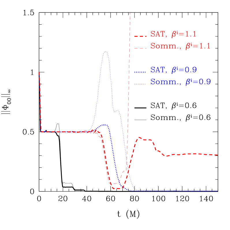
Figure 1: The evolution of $\phi$ for flat-space wave equations with a constant shift in the $x$-direction. As initial data we have used a spherical Gaussian pulse of amplitude $1.0$ and width $1.0$, on a grid $8$ ($121$ grid points) units in size. Thin lines are the Sommerfeld-type boundary conditions without the SAT terms applied, whereas thick lines use the SAT boundary treatment given by Eq. (49).

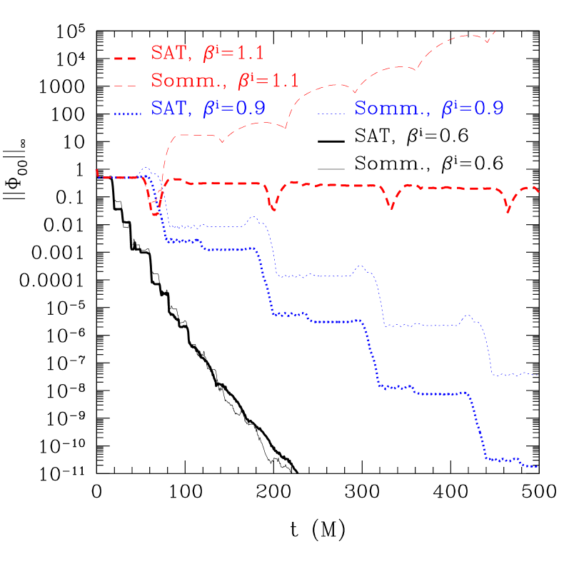
Figure 2: The same as in Fig. 1 but shown in a logarithmic scale for $||\Phi_{00}||_{\infty}$ and on a longer timescale. Note that standard Sommerfeld boundary conditions are unstable for $|\beta^{i}|>1$.

The boundary prescription described in the previous section has been implemented for our harmonic Einstein evolution code ([13] and Sec. 2). We have carried out tests comparing three boundary configurations. The first, which we refer to as “standard Sommerfeld” simply applies Eq. 25 to each evolution variable on each face of the cubical evolution domain, which was the boundary implementation used in [13]. The second (“SAT”) applies the boundary treatment derived in Sec. 3.1, and the third (“CP-SAT”) improves on this by implementing the constraint preserving conditions of Sec. 3.2. We find that in each case, the SAT and CP-SAT boundary conditions respectively improve on the standard Sommerfeld condition in their ability to reduce boundary reflections and constraint violations over time.

4.1 Shifted waves

As a first test of the methodologies outlined in the previous section, we consider a simplified non-relativistic example problem which demonstrates the effectiveness of the SAT method. One of the challenges of designing boundary treatments which control the energy growth for black hole space-times in commonly used gauges is the problem of non-zero shift. A useful problem which has been used as a toy model for the full Einstein equations is the shifted scalar wave equation [27, 20],

$$\left(\partial_{t}^{2}-2\beta^{i}\partial_{i}\partial_{t}-\left(\delta^{ij}-\beta^{i}\beta^{j}\right)\partial_{i}\partial_{j}\right)\phi=0\,,$$ (36)

with shift vector $\beta^{i}=g^{it}/g^{tt}$ (see Eq. (40)). In the appendix, we have explicitly derived the boundary treatment of this problem, which has been implemented in a 3D evolution code.

In Fig. 1, we display results from evolutions of a Gaussian wave packet, for various constant values of the shift. The $L_{\infty}$-norm of the energy of the solution is plotted as a function of time for evolutions using standard Sommerfeld type conditions, Eq. (25), and compared with the SAT conditions derived in Sec. 3.1. As the waveform impinges on the boundary, there is a certain amount of unphysical reflection, but the energy is largely removed from the grid in steps corresponding to the crossing time, as visible in Fig. 2. The boundary reflections are much lower in the case of the SAT boundary conditions, and the evolution is stable even to superluminal, $|\beta^{i}|>1$, shifts suggesting that our conditions are stable even for outflow boundaries.

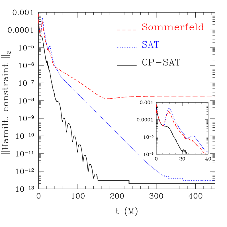
Figure 3: The $L_{2}$-norm of the Hamiltonian constraint for a Teukolsky wave, comparing our constraint-preserving boundary conditions with the standard non-SBP Sommerfeld conditions, as well as the purely Sommerfeld SAT algorithm to ensure well-posedness.

4.2 Linear waves

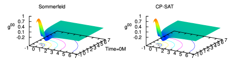
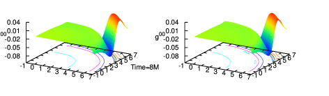
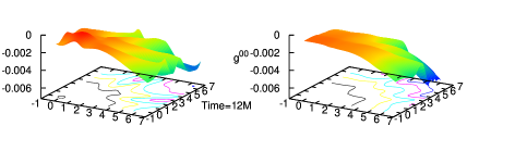
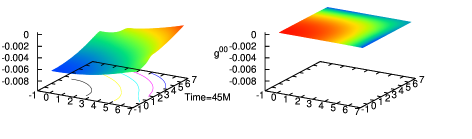
Figure 4: The $tt$ component of the metric for a Brill wave of amplitude $a=0.5$, comparing constraint-preserving boundary conditions with the standard Sommerfeld conditions. The above plot shows a two-dimensional cut in the xy plane at various times. On the right is the evolution of the brill wave with constraint-preserving SAT and on the left is the same simulation but with standard Sommerfeld type boundary conditions.

As a first test of the implementation of the constraint preserving boundary conditions for the full Einstein equations, we have considered low amplitude wave solutions of the linearized Einstein system. These solutions exhibit non-trivial dynamics which exercise the boundaries, but for which the source terms of the Einstein equations are negligible. The particular initial data which we use are the quadrupole Teukolsky waves [28], which have been used as a testbed in a number of numerical studies[29, 30, 31, 32]. The particular solution which we use follows Eppley [33] in combining in-going and outgoing wave packets so as to produce a solution which is regular everywhere in the space-time.

The overall behaviour of the evolutions using our three boundary conditions is summarized in Fig. 3, which plots the evolution of the $L_{2}$-norm of the Hamiltonian constraint as a function of coordinate time, for a wave of amplitude $0.001$. In each case, there is a reduction of the constraint violation as the wave propagates off the grid. In the standard Sommerfeld case, this quickly saturates at a level of $10^{-7}$, determined by the finite differencing resolution. In the case of the SAT boundary conditions, however, the constraint violation eventually reaches machine round-off due to the constraint damping in the interior of the domain. This happens at a much faster rate for the explicitly constraint preserving condition (“CP-SAT”) which introduces the modification described in Sec. 3.2. It is notable that in this case, the initial boundary reflection which the standard Sommerfeld condition shares with the simple SAT treatment, is also absent.

4.3 Nonlinear waves

The goal of our boundary treatment is to reduce the errors introduced into the evolution domain during evolutions of strong field space-times involving non-linear waves, as for instance, generated during binary black hole evolutions. To model this problem in a simplified setting which does not involve complications due to excision or interior mesh-refinement boundaries, we have carried out tests using the nonlinear Brill wave solutions [34]. These solutions have been studied in a number of numerical contexts, both as testbeds, as well as exploring the onset of black hole formation [35, 33, 36, 37, 38]. The initial spatial metric takes the form

$$ds^{2}=\Psi^{4}[e^{2q}(d\rho^{2}+dz^{2})+\rho^{2}d\phi^{2}],$$ (37)

in cylindrical $(\rho,\phi,z)$ coordinates. We choose $q$ of the form of a Gaussian packet centered at the origin,

$$q=a\rho^{2}e^{-r^{2}},$$ (38)

where $a$ is a parameter which is used to set the overall amplitude of the axisymmetric wave. Generally we choose a value of $a=0.5$ to construct a wave which is strong, but not so as to evolve to a black hole. As a result, we expect the initially nonlinear solution generate waves which propagate off the grid leaving behind a flat space-time.

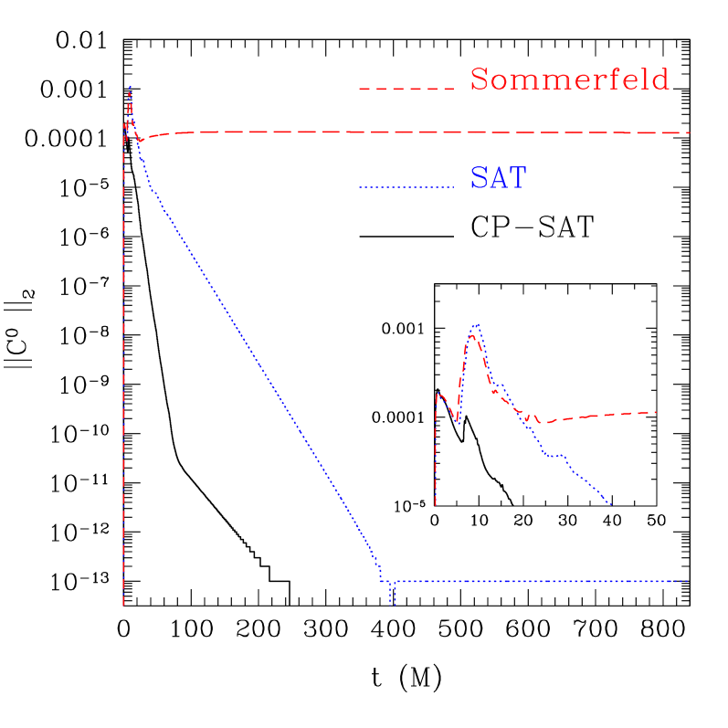
Figure 5: The $L_{2}$-norm of the harmonic constraints for a Brill wave of amplitude $0.5$, comparing constraint-preserving boundary conditions with the standard Sommerfeld conditions, as well as the purely Sommerfeld SAT algorithm to ensure well-posedness.

In Fig. 4 we show a number of frames from two evolutions, displaying the metric $\gamma^{tt}$ component at various time instances on a grid $7$ units in size. In the right column, the standard Sommerfeld conditions have been used, whereas on the left we have used the constraint preserving SAT boundary conditions. By the second frame at $t=8$, the wave pulse has reached the boundary, and the following frames show the reflected pulse. Qualitatively, the CP-SAT boundary conditions show a much smoother profile, with smaller amplitude features. By $t=45$, the wave has left the grid in the CPSBP case, to the extent that it cannot be seen on the linear scale of the figure. In the standard Sommerfeld case, however, there is still some non-trivial dynamical evolution. A more quantitative demonstration is shown in Fig. 5, which plots the $L_{2}$-norm of the harmonic constraint $C^{0}$ as a function of coordinate time for three situations: The standard Sommerfeld boundary conditions (“Sommerfeld”), the SAT boundary conditions developed in Sec. 3.1 (“SAT”), and the constrained version of these boundary conditions, following the prescription of Sec. 3.2 (“CP-SAT”). In the Sommerfeld case, the constraint violation is entirely reflected by the grid boundaries, and the value remains essentially constant at its initial value throughout the evolution of the evolution, even though constraint damping has been used on the interior code. The SAT boundary conditions, however, do a much better job of removing constraint violation from the grid, showing the exponential decrease with time that is expected from the damped solution. The constraint preserving boundary conditions show the strongest damping, suggesting that the constraint violating modes introduced by these boundary conditions are much smaller than for the SAT case. The evolution of the other constraint components show the same behaviour.

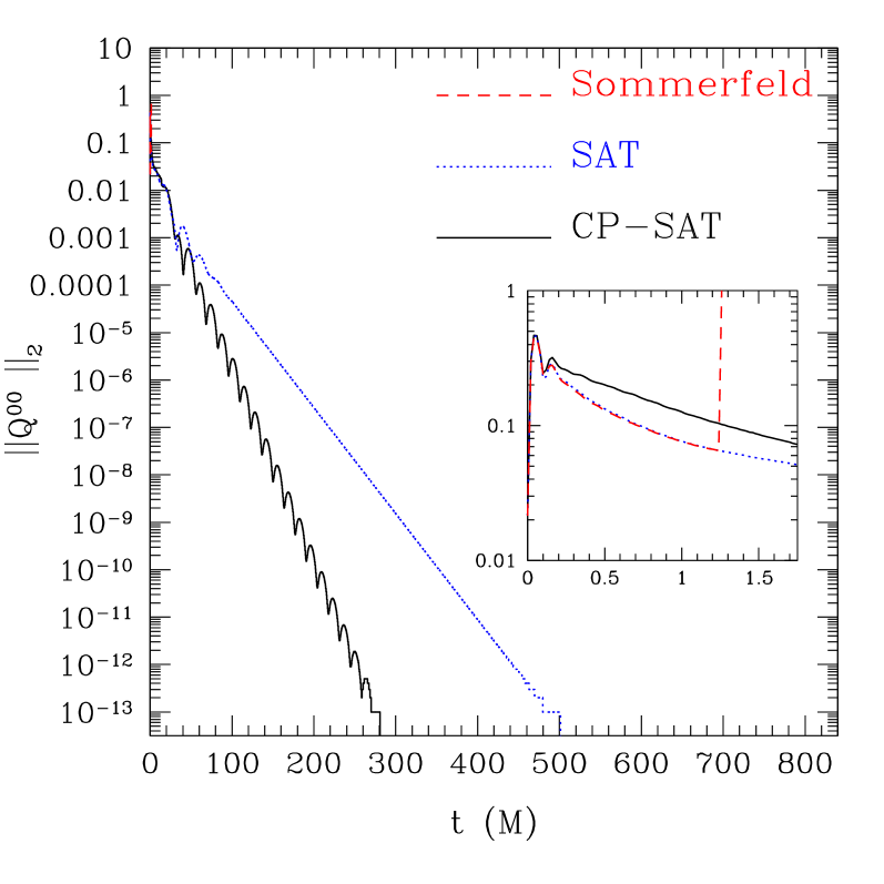
Figure 6: Evolution of $Q^{00}$ component of the harmonic data for a Brill wave perturbed by random noise of a kernel amplitude of $\epsilon\pm 0.075$, over all the grid points. This is placed on top of Brill wave initial data with an amplitude of $a=0.5$.

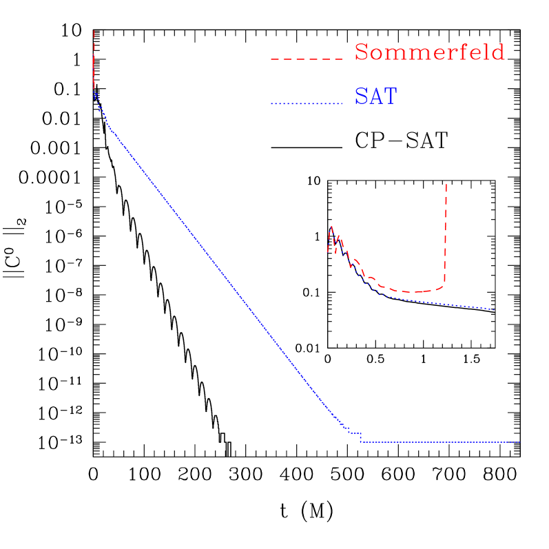
Figure 7: Evolution of the $L_{2}$-norm of the harmonic constraints for a Brill wave ($a=0.5$) perturbed by a checkerboard noise pattern of amplitude $\epsilon\pm 0.1$, over all the grid points, in order to excite the highest frequency grid mode.

As a final test of the stability of our boundary prescription, we have carried out evolutions of Brill waves for which we have attempted to excite high-frequency error modes along the lines of the “robust stability” test [39, 40]. This test is a means of determining whether it is possible for modes of any frequency within any of the grid variables to exhibit exponential growth during the evolution. On a numerical grid, error modes exist at fixed frequencies, set by the grid resolution, and the standard test consists of perturbing each variable at each grid point by a small amount of randomly determined amplitude $\epsilon$. The effect of the random perturbation is to seed modes which then have the potential to grow, if the system is unstable at that frequency. Since being first used in [40] and proposed as a standard testbed in [39], the test has been used in a number of applications to demonstrate well-posedness of numerical implementations [41, 42, 3, 40, 43, 44]. In Fig. 6 we applied this test by applying some kernel of random data to all points including the boundary points. For the SAT methods the random noise gets damped and then the decay of the energy looks similar to that of the standard brill test in Fig. 5. For the standard Sommerfeld boundary conditions the evolution becomes unstable at the boundaries.

A variant of this test recognizes that in the case of an ill-posed system, the fastest exponential growth will result from the highest frequency mode. On a finite-difference grid, the frequency of this mode is set by the grid spacing. We can excite this mode by adding perturbations to the data in a “checkerboard” pattern, where neighboring points receive an opposite perturbation of fixed amplitude $\epsilon$. That is, we choose

$$\epsilon_{ijk}=\left\{\begin{array}[]{ll}+\epsilon,&\textrm{for $i+j+k$ even},\\ -\epsilon,&\textrm{for $i+j+k$ odd.}\end{array}\right.$$ (39)

In Fig. 7 we show the evolution of the $L_{2}$-norm of the $C^{0}$ constraint component for the evolution of an $a=0.5$ Brill wave for which each component of the initial data has been modified according to Eq. (39) with $\epsilon=0.1$. The two versions of the SAT boundary conditions prove to be rather impervious to the initial data perturbation, and display essentially the same behaviour as in the unperturbed case, Fig. 5. It is perhaps notable that the non-constraint-persevering boundary conditions show a slightly slower decay rate than for the non-perturbed data of Fig. 5, so that it takes more than $100$ time units to reach the level of machine round-off, whereas the constraint preserving boundary conditions reach this level in essentially the same amount of time as in the unperturbed case (though with a somewhat different decay profile). The simple Sommerfeld boundary conditions, however, are unable to cope with the initial perturbation and lead to an instability on a very short timescale.

5 Conclusions

We have examined the initial boundary value problem for the second-order formulation of the Einstein equations in the generalized harmonic gauge. The system of evolution equations for this finite-difference harmonic code was derived in [13] where it was shown to be accurate, stable, and convergent for long-term evolutions of black hole space-times, such as head-on collisions of two black holes, isolated black holes, and binary black hole inspiral and merger. In this paper we described the derivation, implementation and testing of a new boundary treatment for this system. We demonstrated that this new treatment maintained the validity and convergence (to lower order) seen with the standard boundary treatments. We additionally show that these conditions give us greater accuracy (for all reasonable resolutions), improved constraint preservation, improved boundary transparency, and greater stability in robust stability tests.

We implemented Sommerfeld-type boundary conditions as in Eq.(25), which are applied via the simultaneous approximation term (SAT) method to control the energy growth of the system, and are designed to be maximally dissipative. We then establish well-posedness for the semi-discrete symmetric hyperbolic evolution system via the energy method [12] by bounding the energy growth of the system under the assumption that the boundaries are in the linearized regime. We have implemented finite-differencing stencils that obey the summation by parts (SBP) rule [11] with the diagonal norm, with minimum bandwidth second-derivative SBP stencils as derived in [24]. These stencils give fourth-order accuracy in the interior, and second-order at the boundary. While the standard stencils give fourth-order everywhere, we show that the improved accuracy of the SBP conditions more than makes up for the loss of two orders of convergence.

The stability and well-posedness of the boundary conditions has been demonstrated for a number of test problems: shifted scalar waves, linearized waves, nonlinear waves, and random and high frequency stability tests. Further improved accuracy results from incorporating the constraint preservation into the conditions, following the prescription of [2, 6]. The boundary conditions are still Sommerfeld type for most metric components, but we substitute conditions gained from enforced preservation of the harmonic constraints. This gives us four conditions directly from the harmonic constraints, three from the coupling of these conditions to our outgoing Sommerfeld-type conditions, and the three components for the directions tangent to each boundary face come only from our Sommerfeld-type conditions. In Sec. 4 we show that, as expected, these new outgoing Sommerfeld, constraint-preserving conditions retain the robust stability and convergence properties of the purely Sommerfeld-SBP conditions. The tests also demonstrate that these new conditions lead to smaller errors in satisfying the constraints, and are more transparent to waves propagating through the boundaries. They should thus lead to more accurate evolutions than the purely Sommerfeld SBP penalty boundary conditions.

In a related study, Rinne et al. [29] have considered a number of boundary treatments for the case of a first-order in space harmonic formulation, including the Kreiss-Winicour [2] treatment adopted here for a second-order system. They find that an additional physically motivated condition, $\partial_{t}\Psi_{0}=0$, which aims to eliminate incoming radiation, can have important effects in reducing physical reflections. Similar modifications may also prove beneficial to the second-order system presented here, though apparent reflections from the outer boundary are rather small even in the case of non-linear waves studied in Sec. 4.3.

With binary black hole evolutions now extending over multiple orbits, and thus many crossing times on conventional computational grids, boundary effects can potentially have a non-trivial influence on the late-time dynamics and extracted gravitational wave signals from such simulations. The tests provided here, including nonlinear Brill wave evolutions, suggest that these methods will also be effective for isolated strong sources, and thus will also be appropriate for black hole space-times, though these involve a number of other technical considerations (such as excision) which we do not explore here. The methods can be extended to other formulations of the Einstein equations, provided certain hyperbolicity assumptions are satisfied, and we are currently pursuing improvements of other commonly used systems such as the conformal-traceless one employed in [25].

References

Appendix

As an instructive example which contains the essential features of the derivation for the Einstein equations, we derive explicitly the energy estimate for the wave equation with shift,

$$\partial_{t}^{2}u=\left(\frac{-\gamma^{ij}}{\gamma^{tt}}\partial_{i}\partial_{j}-2\frac{\gamma^{it}}{\gamma^{tt}}\partial_{i}\partial_{t}\right)u.$$ (40)

where $-\frac{\gamma^{it}}{\gamma^{tt}}$ is the shift $\beta^{i},$ and $\beta^{i}\beta^{j}-\frac{\gamma^{ij}}{\gamma^{tt}}$ is the lapse.

We need to ensure that the energy, $\mathcal{E}^{\left(n\right)}=\|u\left(\cdot,t\right)\|^{2},$ satisfies that the energy of the system is bounded for the duration of the simulation. The time derivative of the energy of the system can be re-written in semi-discrete form as follows:

$$\frac{d}{dt}\mathcal{E} = \frac{d}{dt}\left(\|{u_{t}}\|^{2}+\left\|{-\frac{\gamma^{ij}}{\gamma^{tt}}u_{i}u_{j}}\right\|\right)$$ (41)

$$= (\langle u_{t},u_{tt}\rangle+\langle u_{tt},u_{t}\rangle)-\frac{\gamma^{ij}}{\gamma^{tt}}(\langle u_{i},u_{jt}\rangle+\langle u_{it},u_{j}\rangle)\,.$$

In this section our notation will follow that: we will use partial derivative symbols for continuum equations and subscripts for semi-discrete derivatives. To ensure that this quantity remains bounded in the semi-discrete case, we determine the energy growth which arises from the application of our boundary conditions, and remove this via the simultaneous approximation term (SAT, or “penalty”) method [24]. We use a discrete second derivative stencil which also obeys SBP and more accurately approximates a second derivative than the wide stencil created from applying our first derivative twice.

Since we use differencing operators which obey the SBP condition, we can make use of Eq. (15) to integrate Eq. (41). For the wave equation, after some algebra, this condition gives

$$\frac{d}{dt}\mathcal{E}=-2\left[\left.\frac{\gamma^{ij}}{\gamma^{tt}}(u_{t}u_{j})\right|_{x_{i}=0}^{x_{i}=N_{i}}+\left.\frac{\gamma^{it}}{\gamma^{tt}}(u_{t}^{2})\right|_{x_{i}=0}^{x_{i}=N_{i}}\right]\,.$$ (42)

That is, the change in energy is determined by fluxes at the boundary points, $x_{i}=0$ and $x_{i}=N_{i}$.

On the boundary faces, we impose a set of conditions which for the moment we write in a generic form

$$\left[\beta_{x_{i}=0}\partial_{t}+\alpha_{x_{i}=0}\partial_{i}+\delta_{x_{i}=0}\right]\left(u-u_{0}\right) = 0$$ (43)

$$\left[\beta_{x_{i}=N}\partial_{t}-\alpha_{x_{i}=N}\partial_{i}-\delta_{x_{i}=N}\right]\left(u-u_{0}\right) = 0$$ (44)

in terms of parameters $\alpha$, $\beta$, and $\delta$ which are indexed according to the grid face. These are substituted into into the estimate, Eq. (42), leading to

$$\qquad\qquad\frac{d}{dt}\mathcal{E}=-2\left[\left.\left(\frac{\alpha_{N_{i}}}{\beta_{N_{i}}}u_{t}^{2}-\frac{\gamma^{it}}{\gamma^{tt}}u_{t}^{2}\right)\right|_{x_{i}=N_{i}}-\left.\left(\frac{\alpha_{0_{i}}}{\beta_{0_{i}}}u_{t}^{2}-\frac{\gamma^{it}}{\gamma^{tt}}u_{t}^{2}\right)\right|_{x_{i}=0}\right]\,,$$ (45)

where $\eta^{i}$ is the normal to the boundary face $i$, and $u_{0}$ are data chosen to be consistent with the initial data. The SAT method allows us to choose values for the free parameters in the boundary terms which conserve the energy in the system. We first write the original shifted wave equation, Eq. (40), in semi-discrete form, explicitly including the boundary terms:

$$\hskip 28.45274ptu_{tt}=-\frac{\gamma^{ij}}{\gamma^{tt}}H^{-1}D^{(2)}_{ij}u-2\frac{\gamma^{it}}{\gamma^{tt}}H^{-1}D^{(1)}_{i}u_{t}+\tau_{0_{i}}H^{-1}E_{0_{i}}(\alpha_{0_{i}}u_{t}+\beta_{0_{i}}S_{i}u+\delta_{0_{i}}u)$$

$$\hskip 54.06006pt+\tau_{N_{i}}H^{-1}E_{N_{i}}(\alpha_{N_{i}}u_{t}+\beta_{N_{i}}S_{i}u+\delta_{N_{i}}u)\,.$$ (46)

The $E_{a}$ are vectors of length $N$ defined as $E_{N_{i}}=(0,0\ldots 0,1)^{\top}$ and $E_{0_{i}}=(1,0\ldots,0)^{\top}$ to be zero everywhere except at the boundary points. $S_{i}$ are sideways blended finite differencing stencils satisfying the SBP property, as described in the previous section.

We determine the time dependence of the energy for this new system in order to derive coefficients $\tau$ for our penalty terms which give a well-posed semi-discrete system. Substituting Eq. (46) into Eq. (41), and once again making use of the SBP property, Eq. (15), we arrive at

$$\hskip 28.45274pt\frac{d}{dt}\mathcal{E}=\left(\tau_{N_{i}}\alpha_{N_{i}}-\frac{\gamma^{it}}{\gamma^{tt}}\right)u_{t}^{\top}E_{N_{i}}u_{t}+2\left(\tau_{0_{i}}\alpha_{0_{i}}+\frac{\gamma^{it}}{\gamma^{tt}}\right)u_{t}^{\top}E_{0_{i}}u_{t}$$

$$\hskip 54.06006pt+2\left(\tau_{N_{i}}\beta_{N_{i}}-\frac{\gamma^{ij}}{\gamma^{tt}}\right)u_{t}^{\top}E_{N_{i}}S_{i}u+2\left(\tau_{0_{i}}\beta_{0_{i}}+\frac{\gamma^{ij}}{\gamma^{tt}}\right)u_{t}^{\top}E_{0_{i}}S_{i}u\,.$$ (47)

The free parameters $\tau_{0}$ and $\tau_{N}$ can be used to eliminate the $u_{t}^{\top}E_{N_{i}}S_{i}u$ terms, by setting $\tau_{0}\beta_{0}=-\gamma^{ij}/\gamma^{tt}$ and $\tau_{N}\beta_{N}=\gamma^{ij}/\gamma^{tt}$. Then, the energy evolves according to

$$\frac{d}{dt}\mathcal{E} = -2\left(\beta_{N_{i}}\frac{\gamma^{it}}{\gamma^{tt}}-\alpha_{N_{i}}\frac{\gamma^{ij}}{\gamma^{tt}}\right)\beta_{N_{i}}^{-1}u_{t}^{\top}E_{N_{i}}u_{t}$$ (48)

$$+2\left(\beta_{0_{i}}\frac{\gamma^{it}}{\gamma^{tt}}-\alpha_{0_{i}}\frac{\gamma^{ij}}{\gamma^{tt}}\right)\beta_{0_{i}}^{-1}u_{t}^{\top}E_{0_{i}}u_{t}=0\,.$$

The last equality is arrived at after some algebra, substituting the boundary conditions, Eq. (43–44), and making use of the original wave equation, Eq. (40).

The resulting semi-discrete evolution equation is given by

$$\qquad u_{tt} = -\frac{\gamma^{it}}{\gamma^{tt}}H^{-1}D^{(1)}_{i}u_{t}-\frac{\gamma^{ij}}{\gamma^{tt}}H^{-1}D^{(2)}_{ij}u-\frac{\gamma^{ij}}{\gamma^{tt}\beta_{0_{i}}}H^{-1}E_{0_{i}}(\alpha_{0_{i}}u_{t}+\beta_{0_{i}}S_{i}u+\delta_{0_{i}}u)$$

$$+\frac{\gamma^{ij}}{\gamma^{tt}\beta_{N_{i}}}H^{-1}E_{N_{i}}(\alpha_{N_{i}}u_{t}+\beta_{N_{i}}S_{i}u+\delta_{0_{i}}u)\,,$$ (49)

which, as a result of the application of the SAT terms, satisfies the energy conservation equation $d\mathcal{E}/dt=0$.

References

- [1] Friedrich H and Nagy G 1999 Commun. Math. Phys. 201 619–655
- [2] Kreiss H O and Winicour J 2006 Class. Quant. Grav. 23 S405–S420 (Preprint gr-qc/0602051)
- [3] Rinne O 2006 Class. Quantum Grav. 23 6275 (Preprint gr-qc/0606053)
- [4] Buchman L T and Sarbach O C A 2006 Class. Quantum Grav. 23(23) 6709–6744 (Preprint gr-qc/0608051)
- [5] Motamed M et al. 2006 Phys. Rev. D 73 124008 (Preprint gr-qc/0604010)
- [6] Babiuc M C, Kreiss H O, and Winicour J 2007 Phys. Rev. D75 044002 (Preprint gr-qc/0612051)
- [7] Mattsson K 2003 J. Sci. Comput. 18 133–153
- [8] Mattsson K and Nordström J 2004 J. Comput. Phys. 199(2) 503–540
- [9] Nordström J, Mattsson K, and Swanson C 2007 J. Comput. Phys. 225(1) 874–890 ISSN 0021-9991
- [10] Kreiss H O and Scherer G 1974 in C D Boor, ed, Mathematical Aspects of Finite Elements in Partial Differential Equations (New York: Academica Press)
- [11] Strand B 1994 J. Comput. Phys. 110 47
- [12] Carpenter M, Nordström J, and Gottlieb D 1999 J. Comput. Phys. 148(2) 341
- [13] Szilagyi B et al. 2007 Class. Quantum Grav. 24 S275–S293 (Preprint gr-qc/0612150)
- [14] Babiuc M C, Szilágyi B, and Winicour J 2006 Phys. Rev. D 73 064017 (Preprint gr-qc/0601039)
- [15] Calabrese G et al. 2003 Commun. Math. Phys. 240 377–395 (Preprint gr-qc/0209017)
- [16] Calabrese G et al. 2003 Class. Quantum Grav. 20 L245–L252 (Preprint gr-qc/0302072)
- [17] Kreiss H O, Reula O, Sarbach O, and Winicour J 2007 (Preprint gr-qc/0707.4188)
- [18] Arnowitt R, Deser S, and Misner C W 1962 in L Witten, ed, Gravitation: An introduction to current research (New York: John Wiley) pp 227–265 (Preprint gr-qc/0405109)
- [19] Friedrich H 1985 Comm. Math. Phys. 100 525–543
- [20] Babiuc M C, Szilágyi B, and Winicour J 2006 Class. Quantum Grav. 23 S319–S342 (Preprint gr-qc/0511154)
- [21] Gundlach C, Martin-Garcia J M, Calabrese G, and Hinder I 2005 Class. Quantum Grav. 22 3767–3774 (Preprint gr-qc/0504114)
- [22] Brodbeck O, Frittelli S, Hübner P, and Reula O A 1999 J. Math. Phys. 40 909–923 (Preprint gr-qc/9809023)
- [23] Reula O 1998 Living Rev. Relativity 1 3 URL http://www.livingreviews.org/lrr-1998-3
- [24] Carpenter M, Gottlieb D, and Abarbanel S 1994 J. Comput. Phys. 111 220–236
- [25] Pollney D et al. 2007 Phys. Rev. D76 124002 (Preprint gr-qc/0707.2559)
- [26] Lindblom L et al. 2006 Class. Quantum Grav. 23 S447–S462 (Preprint gr-qc/0512093)
- [27] Calabrese G and Gundlach C 2006 Class. Quant. Grav. 23 S343–S368 (Preprint gr-qc/0509119)
- [28] Teukolsky S A 1982 Phys. Rev. D 26 745–750
- [29] Rinne O, Lindblom L, and Scheel M A 2007 Class. Quantum Grav. 24(16) 4053–4078 (Preprint gr-qc/0711.2084)
- [30] Rezzolla L et al. 1998 Phys. Rev. D 57 1084–1091
- [31] Abrahams A M et al. 1998 Phys. Rev. Lett. 80 1812–1815 (Preprint gr-qc/9709082)
- [32] Rezzolla L et al. 1999 Phys. Rev. D 59 064001 (Preprint gr-qc/9807047)
- [33] Eppley K R 1979 in L Smarr, ed, Sources of gravitational radiation (Cambridge, England: Cambridge University Press) p 275
- [34] Brill D S 1959 Ann. Phys. (N. Y.) 7 466–483
- [35] Eppley K R 1977 Phys. Rev. D 16(6) 1609–1614
- [36] Holz D, Miller W, Wakano M, and Wheeler J 1993 in B L Hu and T A Jacobson, eds, Directions in General Relativity: Proceedings of the 1993 International Symposium, Maryland; Papers in honor of Dieter Brill (Cambridge, England: Cambridge University Press) p 339
- [37] Alcubierre M et al. 2000 Phys. Rev. D 61 041501 (R) (Preprint gr-qc/9904013)
- [38] Pazos E et al. 2007 Class. Quantum Grav. 24(12) S341–S368 (Preprint gr-qc/0612149)
- [39] Alcubierre M et al. 2004 Class. Quantum Grav. 21 589 (Preprint gr-qc/0305023)
- [40] Szilágyi B, Gomez R, Bishop N T, and Winicour J 2000 Phys. Rev. D 62 104006 (Preprint gr-qc/9912030)
- [41] Apples With Apples: Numerical Relativity Comparisons and Tests URL http://www.ApplesWithApples.org/
- [42] Alcubierre M et al. 2004 Class. Quantum Grav. 21(2) 589–613 (Preprint gr-qc/0305023)
- [43] Szilágyi B, Schmidt B, and Winicour J 2002 Phys. Rev. D 65 064015 (Preprint gr-qc/0106026)
- [44] Calabrese G, Hinder I, and Husa S 2006 J. Comput. Phys. 218(2) 607–634 ISSN 0021-9991 (Preprint gr-qc/0503056)