Closed-Orbit Theory of Spatial Density Oscillations in Finite Fermion Systems

Abstract

We investigate the particle and kinetic-energy densities for $N$ non-interacting fermions confined in a local potential. Using Gutzwiller’s semi-classical Green function, we describe the oscillating parts of the densities in terms of closed non-periodic classical orbits. We derive universal relations between the oscillating parts of the densities for potentials with spherical symmetry in arbitrary dimensions, and a “local virial theorem” valid also for arbitrary non-integrable potentials. We give simple analytical formulae for the density oscillations in a one-dimensional potential.

Introduction.— Finite systems of fermions are studied in many branches of physics, e.g., electrons in atoms, molecules, and quantum dots; protons and neutrons in atomic nuclei; or fermionic atoms in traps. Common to these systems are pronounced shell effects which result from the combination of quantized energy spectra with the Pauli exclusion principle. The shell effects manifest themselves most clearly in ionization (or separation) energies and total binding energies. They lead to “magic numbers” of particles in particularly stable species, when degenerate shells or approximately degenerate bunches of single-particle levels are filled. Shell effects appear also in spatial particle densities ks ; thto and kinetic-energy densities. Near the center of a system, the alternating parities of the occupied shells lead to regular quantum oscillations, while the so-called “Friedel oscillations” characteristically appear near the surface of a sufficiently steep confining potential. Kohn and Sham ks analyzed both oscillations in the particle density using Green functions in the one-dimensional WKB approximation. Thouless and Thorpe thto extended their method to give analytical results also for the central oscillations in three-dimensional systems with radial symmetry.

In the periodic orbit theory (POT) gutz ; babl ; poch , semi-classical “trace formulae” allow one to relate the level density of a quantized Hamiltonian system to the periodic orbits of the corresponding classical system. This can be used to interpret quantum shell effects occurring in finite fermion systems in terms of the shortest periodic orbits (see Ref. book for an introduction to POT and applications to various branches of physics). To our knowledge, no attempt has been made so far to interpret quantum oscillations of spatial densities in terms of classical orbits. In the present paper, we use the semi-classical Green function of Gutzwiller gutz to derive analytical expressions for the oscillating parts of particle and kinetic-energy densities in terms of closed non-periodic classical orbits.

General framework.— We consider a $D$-dimensional system of $N$ non-interacting particles with mass $m$, which obey Fermi-Dirac statistics and are bound by a local potential $V({\bf r})$. Note that $V({\bf r})$ can be the self-consistent mean field of an interacting fermion system (such as a nucleus). The energy eigenvalues $E_{n}$ and eigenfunctions $\psi_{n}({\bf r})$ are given by the stationary Schrödinger equation. The particle density of the system at zero temperature, ignoring the spin degeneracy, is given by

$$\rho({\bf r})=\sum_{E_{n}\leq\lambda(N)}\psi_{n}^{\star}({\bf r})\psi_{n}({\bf r})\,,$$ (1)

where the Fermi energy $\lambda(N)$ is determined by normalizing the density to the given particle number $N$. For the kinetic-energy density we discuss two different forms

$$\tau({\bf r}) = -\frac{\hbar^{2}}{2m}\sum_{E_{n}\leq\lambda}\psi_{n}^{\star}({\bf r})\nabla^{2}\psi_{n}({\bf r})\,,$$ (2)

$$\tau_{1}({\bf r}) = \frac{\hbar^{2}}{2m}\sum_{E_{n}\leq\lambda}|\nabla\psi_{n}({\bf r})|^{2}\,,$$ (3)

which after integration both lead to the exact total kinetic energy. We rewrite the above densities in the form

$$\rho({\bf r}) = -\frac{1}{\pi}\,\Im m\int_{0}^{\lambda}{\rm d}E\,G(E,{\bf r},{\bf r}^{\prime})|_{{\bf r^{\prime}}={\bf r}}\,,$$ (4)

$$\tau({\bf r}) = \frac{\hbar^{2}}{2\pi m}\,\Im m\int_{0}^{\lambda}{\rm d}E\,\nabla^{2}_{{\bf r}^{\prime}}G(E,{\bf r},{\bf r}^{\prime})|_{{\bf r}^{\prime}={\bf r}}\,,$$ (5)

$$\tau_{1}({\bf r}) = -\frac{\hbar^{2}}{2\pi m}\,\Im m\int_{0}^{\lambda}{\rm d}E\,\nabla_{{\bf r}}\nabla_{{\bf r}^{\prime}}G(E,{\bf r},{\bf r}^{\prime})|_{{\bf r}^{\prime}={\bf r}}\,,\ \ \ \$$ (6)

where $G(E,{\bf r},{\bf r}^{\prime})$ is the Green function in the energy representation

$$G(E,{\bf r},{\bf r}^{\prime})=\sum_{n}\frac{\psi_{n}^{\star}({\bf r})\psi_{n}({\bf r}^{\prime})}{E+i\epsilon-E_{n}}\,,\quad(\epsilon>0)\,,$$ (7)

and the identity $\displaystyle 1/(E+i\epsilon-E_{n})={\cal P}[1/(E-E_{n})]-i\pi\delta(E-E_{n})$ is used (${\cal P}$ is the Cauchy principal value).

To obtain semi-classical expressions, we replace the Green function by Gutzwiller’s approximation gutz

$$G_{scl}(E,{\bf r,r^{\prime}})=\alpha_{{}_{D}}\!\!\sum_{\rm cl.trj.}\!\!\!\sqrt{|{\cal D}|}\,e^{\frac{i}{\hbar}S(E,{\bf r,r^{\prime}})-i\mu\frac{\pi}{2}},$$ (8)

which is valid to leading order in $1/\hbar$ in the semi-classical limit $\hbar\to 0$, i.e., when the dominating classical actions $S(E,{\bf r,r^{\prime}})$ are large compared with $\hbar$. In Eq. (8), ${\cal D}$ is the Van Vleck determinant given below, $\mu$ is the Morse index and $\alpha_{{}_{D}}=2\pi(2i\pi\hbar)^{-(D+1)/2}$. The sum is over all classical trajectories starting at ${\bf r}$ and ending at ${\bf r^{\prime}}$. The action integral along each trajectory is

$$S(E,{\bf r,r^{\prime}})=\int_{\bf r}^{\bf r^{\prime}}\!\!{\bf p}({\bf r^{\prime\prime}})\cdot{\rm d}{\bf r^{\prime\prime}}.$$ (9)

Since we have to use ${\bf r}={\bf r^{\prime}}$ in (4) - (6), only closed trajectories starting and ending at the same point ${\bf r}$ have to be included in the sum of (8). Following Gutzwiller gutz , we use for each trajectory a local coordinate system ${\bf r}=(q,{\bf r}_{\bot})=(q,r_{\bot 1},r_{\bot 2},\dots,r_{\bot(D-1)})$, whose first variable $q$ is chosen along the trajectory, while the vector ${\bf r}_{\bot}$ of the remaining $D-1$ variables is transverse to it. The Van Vleck determinant then becomes

$${\cal D}=\frac{(-1)^{D}\,m^{2}\,{\cal D}_{\bot}}{p(E,{\bf r})\,p(E,{\bf r^{\prime}})},\qquad{\cal D}_{\bot}=\det(\partial{\bf p^{\prime}}_{\!\!\bot}/\partial{\bf r}_{\!\bot})\,,$$ (10)

where ${\bf p}(E,{\bf r})=\dot{{\bf r}}\left|\!\sqrt{2m[E-V({\bf r})]}\right|\!/|{\dot{\bf r}}|$ is the classical momentum and $p(E,{\bf r})=m\,\dot{q}(E,{\bf r})$ its modulus.

We now want to keep only the leading-order terms in the semi-classical expansion parameter $\hbar$. To this purpose it is useful to decompose the Fermi energy into a smooth and an oscillating part: $\lambda=\widetilde{\lambda}+\delta\lambda$. Assuming that $\delta\lambda\ll\widetilde{\lambda}$, one can show clmr that

$$\delta\lambda=-\int_{0}^{\widetilde{\lambda}}\!\delta g(E)\,{\rm d}E\,/\,\widetilde{g}(\widetilde{\lambda})\,,\quad\int_{0}^{\widetilde{\lambda}}\widetilde{g}(E)\,{\rm d}E=N\,,$$ (11)

where $\widetilde{g}(E)$ is the smooth part of the level density and $\delta g(E)$ its oscillating part, semi-classically given by a sum over the periodic orbits of the classical system gutz .

The sum over closed trajectories to be used in (4) - (6) can be separated into a sum over periodic orbits (POs) and a sum over non-periodic orbits (NPOs). The actions along the POs are independent of ${\bf r}$; their contributions are therefore smooth functions, given only by the initial and final momenta ${\bf p}={\bf p}(E,{\bf r})$ and ${\bf p^{\prime}}={\bf p}(E,{\bf r^{\prime}})$. To lowest order in $\hbar$, the semi-classical densities are given by the POs with zero length. They are identical with the smooth Thomas-Fermi (TF) densities marc , like it is known bm for the level density $\widetilde{g}(E)=g_{TF}(E)$. To next order in $\hbar$, the sums over all NPOs yield the density oscillations, so that the semi-classical particle density has the form

$$\rho_{scl}({\bf r})=\rho_{TF}({\bf r})+\delta\rho({\bf r})\,.$$ (12)

Analogous forms hold for $\tau({\bf r})$ and $\tau_{1}({\bf r})$

For the kinetic-energy densities we have to derive the Green function (8) twice according to (5,6). The semi-classically leading terms come from the derivatives of $S(E,{\bf r,r^{\prime}})$, for which the relations $\nabla_{{\bf r^{\prime}}}S(E,{\bf r,r^{\prime}})={\bf p^{\prime}}$ and $\nabla_{{\bf r}}S(E,{\bf r,r^{\prime}})=-{\bf p}$ hold. The energy integration in Eqs. (4) - (6) can be done by parts. The leading-order results come from the upper integration limit, taken as $\widetilde{\lambda}$. The lower limit, which must be taken to be $V({\bf r})$ since in the semi-classical approximation one has to stay in the classically allowed region, gives no contributions. We then obtain for the oscillating parts of the densities:

$$\delta\rho({\bf r}) = \frac{m\hbar}{\pi}\,\Re e\ \alpha_{{}_{D}}\!\sum_{\rm NPO}\frac{\sqrt{|{\cal D}_{\bot}|}_{{\bf r^{\prime}}={\bf r}}}{p(\widetilde{\lambda},{\bf r})\,T(\widetilde{\lambda},{\bf r})}\,e^{i\Phi(\widetilde{\lambda},{\bf r})},$$ (13)

$$\delta\tau({\bf r}) = \frac{\hbar}{2\pi}\,\Re e\ \alpha_{{}_{D}}\!\sum_{\rm NPO}\frac{p(\widetilde{\lambda},{\bf r})\sqrt{|{\cal D}_{\bot}|}_{{\bf r}^{\prime}={\bf r}}}{T(\widetilde{\lambda},{\bf r})}\,e^{i\Phi(\widetilde{\lambda},{\bf r})},$$ (14)

$$\delta\tau_{1}({\bf r}) = \frac{\hbar}{2\pi}\,\Re e\ \alpha_{{}_{D}}\!\!\sum_{\rm{NPO}}\!\frac{\!\{({\bf p}\!\cdot\!{\bf p^{\prime}})_{\lambda}\!\sqrt{|{\cal D}_{\bot}|}\}_{{\bf r}^{\prime}={\bf r}}}{p(\widetilde{\lambda},{\bf r})\,T(\widetilde{\lambda},{\bf r})}\,e^{i\Phi(\widetilde{\lambda},{\bf r})}\!,~{}~{}~{}~{}$$ (15)

where $({\bf p}\cdot{\bf p^{\prime}})_{\lambda}={\bf p}(\widetilde{\lambda},{\bf r})\cdot{\bf p}(\widetilde{\lambda},{\bf r^{\prime}})$, the phase function in the exponents is $\Phi(\widetilde{\lambda},{\bf r})=S(\widetilde{\lambda},{\bf r,r})/\hbar-\mu\frac{\pi}{2}$, and $T(\widetilde{\lambda},{\bf r})={\rm d}S(E,{\bf r,r})/{\rm d}E|_{E=\widetilde{\lambda}}$. Since the modulus $p$ depends only on position and Fermi energy, but not on the orbits, we can take it outside the sum over the NPOs. We thus immediately find the general relation

$$\delta\tau({\bf r})=[\widetilde{\lambda}-V({\bf r})]\,\delta\rho({\bf r})\,.$$ (16)

It holds for arbitrary, integrable or non-integrable, local potentials in arbitrary dimensions. Eq. (16) may be termed a “local virial theorem” because it relates kinetic and potential energy densities locally at any point. For $\delta\tau_{1}({\bf r})$ we have no such relation, since it depends on the relative directions of final and initial momentum of each orbit. Due to the semi-classical nature of our approximation, Eq. (16) and the results derived below are expected to be valid in the limit of large particle numbers $N$.

One-dimensional systems.— For the further development we now focus on one-dimensional systems characterized by a smooth binding potential $V(x)$ with a minimum at $x=0$. We will explicitly derive a semi-classical expression for the particle density $\rho(x)$; analogous results for the kinetic densities are found in the same way.

The classical motion at fixed energy $E$ is limited by the turning points $x_{\pm}(E)$ defined by $V(x_{\pm})=E$, with $x_{+}(E)>0$ and $x_{-}(E)<0$. In one dimension there are only two types of trajectories going from $x$ to $x^{\prime}$: the first type has its momenta at the initial and final points in the same direction, while for the second type they go in opposite directions. Without loss of generality we may choose $x_{-}\leq x\leq x^{\prime}\leq x_{+}$. The shortest trajectory of the first type goes from $x$ directly to $x^{\prime}$ without reaching any of the turning points; it is indexed by the subscript ’0’ and has the action

$$S_{0}(E,x,x^{\prime})=S(E,0,x^{\prime})-S(E,0,x)\,.$$ (17)

All other trajectories of the first type bounce $j=1,2,\dots$ times forth and back between the turning points before reaching $x^{\prime}$; they are indexed by ’1’ and have the actions

$$S_{1\pm}(E,x,x^{\prime})=j\,S_{1}(E)\pm S_{0}(E,x,x^{\prime})\,,\quad(j=1,2,\dots)$$ (18)

where $S_{1}(E)$ is the action of the primitive periodic orbit and the sign $\pm$ refers to the starting direction. The trajectories of the second type bounce $k=0,1,\dots$ times forth and back before reaching $x^{\prime}$; they are indexed by ’2’ and have the actions

$$S_{2\pm}(E,x,x^{\prime}) = kS_{1}(E)+2S_{\mp}(E)\!\!\!\!\!\!$$

$$\pm [S(E,0,x^{\prime})+S(E,0,x)]\,,\;\;(k=0,1,\dots\!)$$

where $S_{-}(E)=S(E,x_{-},0)$ and $S_{+}(E)=S(E,0,x_{+})$. For a symmetric potential with $V(x)=V(-x)$, one has $S_{-}(E)=S_{+}(E)=S_{1}(E)/2$. From (10) we have $\sqrt{|{\cal D}(E,x,x)|}=m/p(E,x)$ for all trajectories. For smooth potentials in one dimension, the Morse index $\mu$ is equal to the number of turning points, which for the above trajectories is $\mu_{0}=0$, $\mu_{1\pm}=2j$, and $\mu_{2\pm}=2k+1$. [For a one-dimensional box with reflecting walls, the Morse index equals twice the number of turning points; our semi-classical densities become exact in this case.]

Using (17–Closed-Orbit Theory of Spatial Density Oscillations in Finite Fermion Systems) and $D$=1 in Eq. (8), we now obtain the semi-classical particle density $\rho_{scl}(x)$ as a sum of the three types of contributions indexed as above:

$$\rho_{scl}(x)=\rho_{0}(x)+\!\sum_{\sigma=+-}\!\![\,\rho_{1\sigma}(x)+\rho_{2\sigma}(x)\,]\,.$$ (20)

Since we have to use $x=x^{\prime}$, the only contributing orbits of type 0 have zero length, those of type 1 are periodic, and those of type 2 are non-periodic. Doing the energy integration by parts, we get to leading-order in $\hbar$

$$\rho_{0}(\lambda,x) = \frac{(2m)^{1/2}}{\pi\hbar}\sqrt{\lambda-V(x)}\,,$$ (21)

$$\rho_{1}(x) = \frac{2m}{\pi}\sum_{j=1}^{\infty}(-1)^{j}\,\frac{\sin\{jS_{1}(\widetilde{\lambda})/\hbar\}}{p(\widetilde{\lambda},x)\,jT_{1}(\widetilde{\lambda})}\,,$$ (22)

where $T_{1}(\widetilde{\lambda})$ is the period of the primitive periodic orbit. Taylor expanding $\rho_{0}(\lambda,x)$ in Eq. (21) around $\widetilde{\lambda}$ yields the well-known TF density, $\rho_{TF}(x)=\rho_{0}(\widetilde{\lambda},x)$, plus a term linear in $\delta\lambda$ which, using Eq. (11), cancels exactly the contribution $\rho_{1}(x)$ in (22). The leading-order oscillating term is therefore given by the type 2 orbits, i.e., by $\delta\rho(x)=\rho_{2+}(x)+\rho_{2-}(x)$ which has the explicit form

$$\delta\rho(x)=-\frac{m}{\pi}\!\sum_{k=0\atop\sigma=\pm}^{\infty}(-1)^{k}\frac{\cos\{[kS_{1}(\widetilde{\lambda})\!+\!R_{\sigma}(\widetilde{\lambda},x)]/\hbar\}}{p(\widetilde{\lambda},x)[kT_{1}(\widetilde{\lambda})+R^{\prime}_{\sigma}(\widetilde{\lambda},x)]},$$ (23)

with $R_{\pm}(\widetilde{\lambda},x)=2S_{\pm}(\widetilde{\lambda})\mp 2S(\widetilde{\lambda},0,x)$. This result is equivalent, although not obviously identical, with the result given in Eq. (3.36) of ks .

For the kinetic-energy densities we proceed in the same way. The smooth parts of $\tau(x)$ and $\tau_{1}(x)$ are identical and equal to the TF kinetic-energy density $\tau_{TF}(x)$; for their oscillating parts we obtain the one-dimensional version of the relation (16) and, in addition, the new relation

$$\delta\tau_{1}(x)=-\delta\tau(x)\,,$$ (24)

which holds due to the opposite initial and final momenta of the NPOs of type 2 which contribute to (15).

In Fig. 1, we test our semi-classical results for the potential $V(x)=x^{4}\!/4$ with $N=40$ particles (with units such that $\hbar=m=1$). The upper panel shows $\delta\rho(x)$ given in (23) by the solid line, while the dots represent the quantum-mechanical expression (1) after subtracting the TF density. The agreement is very good except close to the classical turning point where the TF approximation breaks down. The lower panel demonstrates the validity of the relations (16) (with ${\bf r}\to x$) and (24). The small deficiencies near the classical turning points can be overcome and the tail in the classically forbidden region described by the standard WKB treatment ks ; thto or the TF-Weizsäcker theory marc .

A simpler form for $\delta\rho(x)$ is found if one restricts oneself to the interior part of the system around $x=0$, where $V(x)\ll\widetilde{\lambda}$. Then the action integral $S(\widetilde{\lambda},0,x)$ can be approximated by $S(\widetilde{\lambda},0,x)\simeq xp_{\lambda}$, where $p_{\lambda}=(2m\widetilde{\lambda})^{1/2}$ is the smooth Fermi momentum. We then obtain

$$\delta\rho(x)=\frac{-2m\cos(2xp_{\lambda}/\hbar+\delta\Phi)}{\pi\,p_{\lambda}\,T_{1}(\widetilde{\lambda})}\,C_{N}(\widetilde{\lambda})\,,$$ (25)

where $\delta\Phi=[S_{-}(\widetilde{\lambda})-S_{+}(\widetilde{\lambda})]/\hbar$ is a phase difference related to the asymmetry of the potential, and

$$C_{N}(\widetilde{\lambda})=\sum_{k=0}^{\infty}(-1)^{k}\frac{\cos\{[(k+1/2)S_{1}(\widetilde{\lambda})]/\hbar\}}{(k+1/2)}\,.$$ (26)

To evaluate this sum, we exploit the fact that the action $S_{1}(\widetilde{\lambda})$ in one dimension can be related to the particle number $N$ by $S_{1}(\widetilde{\lambda})\approx 2\pi\hbar N$, which is nothing but the well-known Bohr-Sommerfeld quantization condition. Using this relation in (26) and the identity $\sum_{k=0}^{\infty}(-1)^{k}\cos[(2k+1)N]/(2k+1)=(-1)^{N}\pi/4$, we find the approximate expression for the central oscillations

$$\delta\rho(x)=(-1)^{N+1}\,\frac{m}{p_{\lambda}T_{1}(\widetilde{\lambda})}\,\cos(2xp_{\lambda}/\hbar+\delta\Phi)\,,$$ (27)

which can also be obtained from Eq. (3.36) in Ref. ks in the limit $V(x)\ll\widetilde{\lambda}$. It is shown by the dashed line in the upper panel of Fig. 1. Using Eqs. (16) and (24) one can give analogous simple results for the kinetic-energy density oscillations near $x=0$.

Our derivation shows that periodic orbits do not contribute to the oscillations in the densities $\rho(x)$, $\tau(x)$ and $\tau_{1}(x)$, while they are known gutz to give the most important contributions to the oscillating level density $\delta g(E)$. In fact, the most important contribution to (23) comes from the two shortest non-periodic orbits which go from $x$ to one of the turning points and back; for small $x$ their action difference is $2xp_{\lambda}$. The summation over all longer non-periodic orbits yields the oscillating sign depending

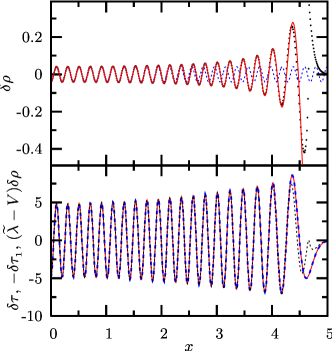
Figure 1: (Color online) Upper panel: Oscillating part $\delta\rho(x)$ of the particle density of $N$=40 fermions in the potential $V(x)=x^{4}\!/4$. Dots show the quantum-mechanical result; the solid line shows the semi-classical result $\delta\rho(x)$ in (23) and the dashed line the approximation (27) for small $x$ values.
Lower panel: Oscillating parts of the quantum-mechanical kinetic-energy densities in the same system: $\delta\tau(x)$ (solid line) and $-\delta\tau_{1}(x)$ (dashed line). The dotted line shows the function $[\widetilde{\lambda}-V(x)]\,\delta\rho(x)$ using the quantum-mechanical $\delta\rho(x)$.

on the particle number $N$. We emphasize that the oscillations in Eq. (27) have the universal wave length $\hbar\pi/p_{\lambda}$ independent on the particular form of the potential $V(x)$.

Higher-dimensional radial systems.— In a forthcoming paper bkmr , we generalize our method for higher-dimensional systems. For binding potentials $V(r)$ with spherical symmetry in $D>1$ dimensions, one can separate two kinds of spatial oscillations in the radial variable:
$(i)$ irregular longer-ranged oscillations, which are attributed to nonlinear classical orbits, and
$(ii)$ regular, rapid oscillations of the kind discussed above and denoted here by $\delta\rho(r)$, $\delta\tau(r)$, and $\delta\tau_{1}(r)$.
The regular rapid oscillations originate from non-periodic linear orbits with zero angular momentum, starting from $r$ in the radial direction and returning with opposite radial momentum to $r$; these orbits correspond exactly to our above type 2 orbits in one dimension. From their contributions to the semi-classical Green function (8) and hence to (13), it is straightforward to derive the following relation, valid to leading order in $\hbar$:

$$-\frac{\hbar^{2}}{8m}\nabla^{2}\delta\rho(r)=[\widetilde{\lambda}-V(r)]\,\delta\rho(r)\,.$$ (28)

Similarly, it follows from the nature of the radial type 2 orbits that $({\bf p}\cdot{\bf p^{\prime}})_{{\bf r}^{\prime}={\bf r}}=-p^{2}$ in (15) and hence the rapid oscillations in the kinetic-energy densities $\tau(r)$ and $\tau_{1}(r)$ fulfill the relation (24) in the radial variable $r$:

$$\delta\tau_{1}(r)=-\delta\tau(r)\,.\vspace*{0.1cm}$$ (29)

For small $r$, where $V(r)\ll\widetilde{\lambda}$, Eq. (28) becomes a universal eigenvalue equation for $\delta\rho(r)$ with eigenvalue $\widetilde{\lambda}$, which can be transformed into the Bessel equation. Its solutions yield the generalization of Eq. (27) (with $\delta\Phi=0$) for the rapid oscillations near $r=0$:

$$\delta\rho(r)=(-1)^{{}^{M\!-1}}\frac{m}{2\hbar\,T_{r1}(\widetilde{\lambda})}\left(\frac{p_{\lambda}}{4\pi\hbar r}\right)^{\!\nu}\!\!J_{\nu}(2rp_{\lambda}/\hbar)\,.$$ (30)

Here $J_{\nu}(z)$ is a Bessel function with index $\nu=D/2-1$, $M$ is the number of filled main shells, and $T_{r1}$ is the period of one radial oscillation. For $D=3$, Eq. (30) agrees with the result of thto up to a $\widetilde{\lambda}$ dependent normalization factor. Our results (16) and (28) - (30) agree with those derived analytically for harmonic oscillator potentials $V(r)=cr^{2}$ in arbitrary dimension $D$ from the quantum-mechanical densities to leading order in a $1\!/N$ expansion brmu . Numerical tests of our semi-classical relations for a variety of systems will be given in Ref. bkmr .

Conclusions.— We have shown that quantum oscillations in spatial densities can be derived without resorting to wave functions, but using the closed non-periodic orbits of the classical system. Our one-dimensional result for $\delta\rho(x)$ is equivalent to that of ks , but its derivation by the summation over classical orbits appears more transparent to us. We note that the semi-classical theory can be easily generalized to grand-canonical systems at finite temperatures temp . Our results may become useful in the analysis of weakly interacting trapped fermionic gases (see, e.g., trapex ) for which the mean-field approximation is appropriate. We present it as a challenge to verify the “local virial theorem” (16) experimentally.

We are grateful to J. D. Urbina for helpful comments and to A. Koch for numerical data used in the figure.

References

- (1) W. Kohn and L. J. Sham, Phys. Rev. 137, A1697 (1965).
- (2) M. A. Thorpe and D. J. Thouless, Nucl. Phys. A 156, 225 (1970).
-
(3)
M. C. Gutzwiller, J. Math. Phys. 12, 343 (1971);
M. C. Gutzwiller: Chaos in Classical and Quantum Mechanics (Springer Verlag, New York, 1990). - (4) R. Balian and C. Bloch, Ann. Phys. (N. Y.) 69, 76 (1972).
- (5) Chaos Focus Issue on Periodic Orbit Theory, ed. by P. Cvitanović: Chaos 2, pp. 1-158 (1992).
- (6) M. Brack and R. K. Bhaduri: Semiclassical Physics (Westview, Boulder, USA, 2003).
- (7) M. Brack and M. V. N. Murthy, J. Phys. A 36, 1111 (2003).
- (8) M. Centelles, P. Leboeuf, A. Monastra, J. Roccia, P. Schuck, and X. Viñas, Phys. Rev. C 74, 034332 (2006).
- (9) N. March, Adv. in Physics 6, 1 (1957).
- (10) M. Berry and K. E. Mount, Rep. Prog. Phys. 35, 315 (1972).
- (11) J. Roccia, A. Koch, M. Brack and M. V. N. Murthy, to be published.
- (12) V. M. Kolomietz, A. G. Magner, V. M. Strutinsky, Sov. J. Nucl. Phys. 29 768 (1979).
- (13) B. DeMarco and D. S. Jin, Science 285, 1703 (1999).