Short-time inertial response of viscoelastic fluids measured with Brownian motion and with active probes

Abstract

We have directly observed short-time stress propagation in viscoelastic fluids using two optically trapped particles and a fast interferometric particle-tracking technique. We have done this both by recording correlations in the thermal motion of the particles and by measuring the response of one particle to the actively oscillated second particle. Both methods detect the vortex-like flow patterns associated with stress propagation in fluids. This inertial vortex flow propagates diffusively for simple liquids, while for viscoelastic solutions the pattern spreads super-diffusively, dependent on the shear modulus of the medium.

I Introduction

Motion in simple liquids at small scales is usually characterized by low Reynolds numbers, in which the response of a liquid to a force applied at one point is Stokes-like—decaying with distance $r$ as $1/r$ away from the origin of the disturbance LandauFluids ; brenner ; Guyon . Here, fluid inertia can be neglected, and the force is effectively felt instantaneously everywhere within the medium. In practice, this is a good approximation, for instance, in water at the colloidal scale up to micrometers on times scales larger than a microsecond. At short times or high frequencies, however, fluid inertia limits the range of stress propagation. Any instantaneous disturbance must be confined to a small region for short times. If the medium is also incompressible, then this naturally gives rise to vorticity and backflow. In simple liquids, stress then propagates through the diffusive spreading of this vortex. Although this basic physical picture has been known theoretically for simple liquids since the work of Oseen in 1927 Oseen and has been shown in computer simulations since the 1960s Alder , experimental observation of these effects have been largely indirect, for instance, in the form of short-time corrections to Brownian motion exper_tails . Direct experimental observation has only recently been possible because of the high temporal and spatial resolution required maryam .

The finite time it takes for vorticity to propagate leads to persistence of fluid motion that manifests itself in algebraic decay of the auto-correlation function of the velocity of either a fluid element or a particle embedded in the fluid. This decay is slower than the naive expectation of exponentially-decaying correlations for a massive particle experiencing viscous drag. Thus, the effect is known as the long time tail effect exper_tails ; theor_tails ; Lukic , which characterizes the transition from ballistic to Brownian motion of particles in simple liquids. This effect has been shown to be present even at the atomic level, e.g., from neutron scattering experiments on liquid sodium Morkel .

We have shown that the inter-particle correlations and response functions of two particles can be used to directly resolve the flow pattern and dynamics of vortex propagation maryam ; liverpool . This was done by measuring the correlated thermal motion of two optically trapped spherical particles using an interferometric technique  detection Gittes ; setup maryam with high temporal (up to 100 kHz) and spatial (sub-nanometer) resolution in both viscous and viscoelastic fluids. We were able to observe, for instance, the anti-correlation in the inter-particle fluctuations of thermal motion that is characteristic of the vortex propagation. The method is related to passive two-particle microrheology  crocker ; Starrs ; meiners ; bartlett ; Gardel ; Koenderink actin which can be used to measure shear elastic moduli of viscoelastic materials.

The inter-particle response functions $\alpha(\omega)$, with real ($\alpha^{\prime}$) and imaginary ($\alpha^{\prime\prime}$) parts defined by $\alpha(\omega)=\alpha^{\prime}(\omega)+i\alpha^{\prime\prime}(\omega)$ are obtained for motion parallel ($\alpha_{||}$) and perpendicular ($\alpha_{\bot}$) to the centerline connecting the two particles. In the passive approach, we directly measure the imaginary part of the response function from the thermal position fluctuations of the two particles via the fluctuation-dissipation theorem (FDT). The real part of the response function is then obtained from a Kramers-Kronig integral MR97 .

Here, in order to directly measure both real (in-phase) and imaginary (out-of-phase) parts of the response function, we have developed an active method  Hough ; Mizuno active , in which one optical trap drives oscillatory motion of one particle, while the response of a second particle is measured at separation $r$. We present and compare detailed experimental results of both passive and active approaches. We also present a theoretical derivation of the predicted response functions and corresponding algebraic decay of the velocity autocorrelation functions for viscoelastic fluids.

The outline of the paper is as follows. In section II, we present the theoretical analysis. In section III, we present the materials and methods of sample preparation, as well as the experimental techniques for the passive and active measurements of the response functions. In section IV we describe our methods of data analysis used for the results presented in section V. In the results section V, we first compare the data for simple liquids with the dynamic Oseen tensor, which demonstrates the diffusive propagation of the vortex flow. We then present our results and comparison with theory for viscoelastic solutions, including the evidence for superdiffusive stress propagation. Finally, we conclude with a discussion (section VI), also mentioning implications of our results for microrheology in general.

II THEORY AND BACKGROUND

Newtonian liquids are described by the Navier-Stokes equation, which is non-linear. The non-linearity, however, can usually be neglected either for small distances or for low velocities LandauFluids ; brenner . This is the so-called low Reynolds number regime, since the relative importance of non-linearities is characterized by the Reynolds number $\mbox{Re}=\frac{UL\rho}{\eta}$, where $U$, $L$, $\rho$, and $\eta$ are, respectively, the characteristic velocity and length scales, the density, and the viscosity. For steady flow, this regime can also be thought of as the non-inertial regime, in which stress propagates instantaneously and, for instance, the velocity response at a distance $r$ from a point force varies as $1/r$ LandauFluids ; brenner ; Guyon . Such Stokes flow accurately describes the motion of micron-size objects in water on time scales longer than a few microseconds.

Even at low Reynolds number, however, there are remaining consequences of fluid inertia for non-stationary flows Guyon . This unsteady Stokes approximation is described by the linearized Navier-Stokes equation:

$$\rho\frac{\partial}{\partial t}\vec{v}=\eta\nabla^{2}\vec{v}-\vec{\nabla}P+\vec{f},$$ (1)

where $\vec{v}$ is the velocity field, $P$ is the pressure that enforces the incompressibility of the liquid and $\vec{f}$ is the force density applied to the fluid. By taking the curl of this equation we observe that the vorticity $\vec{\Omega}=\vec{\nabla}\times\vec{v}$ satisfies the diffusion equation with diffusion constant $\nu=\eta/\rho$.

As noted above, the short-time response of a liquid to a point force generates a vortex. The propagation of stress away from the point disturbance is diffusive: after a time $t$, this vortex expands away from the point force to a size of order $\delta\sim\sqrt{\eta t/\rho}$. In the wake of this moving vortex is the usual Stokes flow that corresponds to a $1/r$ dependence of the velocity field. For an oscillatory disturbance at frequency $\omega$, the propagation of vorticity defines a penetration depth $\delta\sim\sqrt{\eta/(\omega\rho)}$ LandauFluids . Stress effectively propagates instantaneously on length scales shorter than this.

This picture generalizes to the case of homogenous viscoelastic media characterized by an isotropic, time-dependent shear modulus $G(t)$ bird , although the propagation of stress generally becomes super-diffusive liverpool . We further assume that the medium is incompressible, which is a particularly good approximation for polymer solutions such as those considered here, at least at high frequencies Brochard ; MR97 ; 2fluid . The deformation of the medium is characterized by a local displacement field $\vec{u}(\vec{r},t)$, and the viscoelastic analogue of the Navier-Stokes equation (1) is:

$$\rho\frac{\partial^{2}}{\partial t^{2}}\vec{u}(\vec{r},t) = \vec{\nabla}\cdot\tensor{\bm{\sigma}}(\vec{r},t)-\vec{\nabla}P+\vec{f}(\vec{r},t)\,,$$ (2)

where

$$\tensor{\bm{\sigma}}(\vec{r},t) = 2\int^{t}_{-\infty}dt^{\prime}G(t-t^{\prime})\tensor{\bm{\gamma}}(\vec{r},t^{\prime})$$ (3)

is the local stress tensor and

$$\tensor{\bm{\gamma}}=\frac{1}{2}\left[\vec{\nabla}\vec{u}+\left(\vec{\nabla}\vec{u}\right)^{\dagger}\right]$$ (4)

is the local deformation tensor. Incompressibility corresponds to the constraint ${\vec{\nabla}\cdot\vec{u}}=0$

Equations (2,3) can be simplified by a decomposition of the force density and deformation into Fourier components. Taking spatio-temporal Fourier Transforms defined as

$$\vec{u}(\vec{k},\omega)=\int d^{3}r\int_{-\infty}^{\infty}dt\,\,e^{i(\omega t-\vec{k}\cdot\vec{r})}\vec{u}(\vec{r},t),$$ (5)

and defining the complex modulus

$$G^{\star}(\omega)\equiv G^{\prime}(\omega)+iG^{\prime\prime}(\omega)=\int_{0}^{\infty}dte^{i\omega t}G(t),$$ (6)

we can eliminate the pressure by imposing incompressibility in Eqs. (2,3). This leads to

$$\vec{u}(\vec{k},\omega)=\left(\frac{{\bf 1}-\hat{k}\hat{k}}{G^{\star}(\omega)k^{2}-\rho\omega^{2}}\right)\cdot\vec{f}(\vec{k},\omega)\,,$$ (7)

where $\hat{k}=\vec{k}/|k|$. We invert this Fourier transform to obtain the displacement response function due to a point force applied at the origin.

II.1 Response functions

For a point force $\vec{f}$ at the origin, the linear response of the medium at $\vec{r}$ is given by a tensor $\alpha_{ij}$, where $u_{i}(\vec{r},\omega)=\alpha_{ij}(\vec{r},\omega)f_{j}(\vec{0},\omega)$. Here, $\alpha_{ij}=\alpha^{\prime}_{ij}+i\alpha^{\prime\prime}_{ij}$ is, in general, complex. Given our assumptions of rotational and translational symmetry, there are only two distinct components of the response. These are (1) a parallel response that is given by a displacement field $\vec{u}$ parallel to both $\vec{f}$ and $\vec{r}$, and (2) a perpendicular response given by $\vec{u}$ parallel to $\vec{f}$ and perpendicular to $\vec{r}$. The parallel response function $\alpha_{\parallel}$, for instance, is obtained from the inverse Fourier transform of Eq. (7) liverpool .

The response functions for general $G^{\star}(\omega)$ are given by

$$\alpha_{\parallel}\left(r,\omega\right)=\alpha_{\parallel}^{\prime}+i\,\alpha_{\parallel}^{\prime\prime}=\frac{1}{4\pi G^{\star}(\omega)r}\chi_{\parallel}\left(r\sqrt{\kappa}\right),$$ (8)

and

$$\alpha_{\perp}\left(r,\omega\right)=\alpha_{\perp}^{\prime}+i\,\alpha_{\perp}^{\prime\prime}=\frac{1}{8\pi G^{\star}(\omega)r}\chi_{\perp}\left(r\sqrt{\kappa}\right),$$ (9)

where $\kappa={\rho\omega^{2}/G^{\star}(\omega)}$ is complex and

$$\chi_{\parallel}\left(x\right)=\frac{2}{x^{2}}\left[\left(1-ix\right)e^{ix}-1\right],$$ (10)

and

$$\chi_{\perp}\left(x\right)=\frac{2}{x^{2}}\left[1+\left(x^{2}-1+ix\right)e^{ix}\right].$$ (11)

The magnitude of $\kappa$ defines the inverse (viscoelastic) penetration depth $\delta$.

II.1.1 Simple liquids

For a simple liquid, $G^{\star}(\omega)=-i\,\omega\eta$ and $\kappa=i\rho\omega/\eta$. The velocity response of the liquid is then characterized by

$$-i\omega\alpha_{\parallel}\left(r,\omega\right)=\omega\alpha_{\parallel}^{\prime\prime}-i\,\omega\alpha_{\parallel}^{\prime}=\frac{1}{4\pi\eta r}\tilde{\chi}_{\parallel}\left(r\sqrt{\frac{\rho\omega}{2\eta}}\right),$$ (12)

and

$$-i\omega\alpha_{\perp}\left(r,\omega\right)=\omega\alpha_{\perp}^{\prime\prime}-i\,\omega\alpha_{\perp}^{\prime}=\frac{1}{8\pi\eta r}\tilde{\chi}_{\perp}\left(r\sqrt{\frac{\rho\omega}{2\eta}}\right),$$ (13)

where

$$\tilde{\chi}_{\parallel}^{\prime}\left(x\right)=\frac{\left[\left(1+x\right)\sin x-x\cos x\right]e^{-x}}{x^{2}},$$

$$\tilde{\chi}_{\parallel}^{\prime\prime}\left(x\right)=\frac{1-\left[\left(1+x\right)\cos x+x\sin x\right]e^{-x}}{x^{2}},$$

$$\tilde{\chi}_{\perp}^{\prime}\left(x\right)=\frac{\left[\left(x+2x^{2}\right)\cos x-\left(1+x\right)\sin x\right]e^{-x}}{x^{2}},$$

$$\tilde{\chi}_{\perp}^{\prime\prime}\left(x\right)=\frac{\left[\left(x+2x^{2}\right)\sin x+\left(1+x\right)\cos x\right]e^{-x}-1}{x^{2}}.$$

(17)

Thus, for instance, the in-phase and out-of-phase velocity response in the parallel direction are given by $\omega\alpha^{\prime\prime}=\frac{1}{4\pi\eta r}\tilde{\chi}^{\prime}_{\parallel}$ and $-\omega\alpha^{\prime}=\frac{1}{4\pi\eta r}\tilde{\chi}^{\prime\prime}_{\parallel}$.

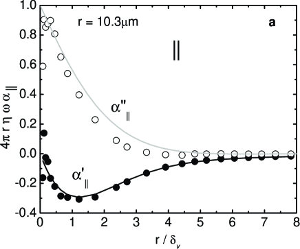
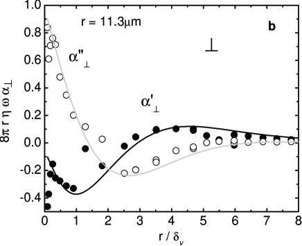
Figure 1: Comparison of theoretical and experimentally measured response functions for a simple liquid. The predictions of the normalized velocity field from the dynamic Oseen tensor in Eqs. (12,13) are shown as black and gray lines. Normalized complex inter-particle response functions between two probe particles (silica beads, $R$ = 0.58 $\mu$m) measured with the active microrheology method in water: (a) $4\pi r\eta\omega\alpha_{||}$ in the parallel direction and (b) $8\pi r\eta\omega\alpha_{\bot}$ in the perpendicular direction, plotted versus the ratio of the separation distance $r$ (fixed for a given bead pair, $r$ = 11.3 $\mu$m for parallel, and $r$ = 10.3 $\mu$m for perpendicular) to the frequency-dependent viscous penetration depth $\delta_{v}$. Both real (filled symbols) and imaginary parts (open symbols) are shown, for both parallel and perpendicular directions. These results are compared with the theory for $\eta$ = 0.97 mPa s and $\rho$ = 1000 kg m^-3. There is good agreement with no free parameters.

We have written the response functions in Eqs. (8, 9) in a form in which the noninertial limits ($x\rightarrow 0$) are simple: $\chi_{\parallel,\perp}\rightarrow 1$. Thus, for a simple liquid in the limit $x\rightarrow 0$, Eqs. (12, 13) reduce to the (time-independent) Oseen tensor brenner ; Oseen . For finite $x$, these response functions give the dynamic Oseen tensor Oseen ; Mazur , which are shown as the solid lines in Fig. 1, where for small $r/\delta$ the parallel and perpendicular velocity response (i.e., $-i\omega\alpha_{\parallel,\perp}$) approach $\frac{1}{4\pi\eta r}$ and $\frac{1}{8\pi\eta r}$ for a unit force at the origin. These then decay for $r\gtrsim\delta$. The region of negative response in the perpendicular case corresponds to the back-flow of the vortex.

The response functions above represent the ensemble-average displacements due to forces acting in the medium. These response functions also govern the equilibrium thermal fluctuations and the correlated fluctuations from point to point within the medium. The relationship between thermal fluctuations and response is described by the Fluctuation-Dissipation theorem. Specifically, for points separated by a distance $r$ along the $\hat{x}$ direction,

$$C_{\parallel,\perp}(r,\omega)=\frac{2k_{B}T}{\omega}\alpha^{\prime\prime}_{\|,\perp}(r,\omega),$$ (18)

where

$$C_{\|}(r,\omega)=\int_{-\infty}^{\infty}dte^{i\omega t}\langle u_{x}(0,0)u_{x}(r,t)\rangle$$ (19)

and

$$C_{\perp}(r,\omega)=\int_{-\infty}^{\infty}dte^{i\omega t}\langle u_{y}(0,0)u_{y}(r,t)\rangle.$$ (20)

II.1.2 Polymer solutions

An experimentally pertinent illustration is given by the high frequency complex shear modulus of a polymer solution,

$$G^{\star}(\omega)=-i\omega\eta+\bar{g}(-i\omega)^{z}=|G|e^{-i\psi}$$ (21)

which has both solvent and polymer contributions. For the Rouse model of flexible polymers $z=1/2$ Doi , while for semiflexible polymers $z=3/4$ MR97 ; Morse98 ; Gittes98 . The latter case is shown as the solid lines in Fig. 2. We see that the oscillatory or anti-correlated response becomes more pronounced in viscoelastic materials.

The magnitude of the complex modulus is given by

$$|G|=\sqrt{\left(\bar{g}\omega^{z}\right)^{2}+\left(\omega\eta\right)^{2}+2\omega^{z+1}\eta\bar{g}\sin\left(\pi z/2\right)},$$ (22)

while its phase is given by

$$\sin\psi=\frac{\left(\omega\eta+\bar{g}\omega^{z}\sin\left(\pi z/2\right)\right)}{|G|}$$ (23)

and

$$\quad\cos\psi=\frac{\bar{g}\omega^{z}\cos\left(\pi z/2\right)}{|G|}\,.$$ (24)

It is also useful to have the following expressions for the half-phase-angles

$$\sin{\psi\over 2} = \sqrt{{1\over 2}\left(1-{\bar{g}\omega^{z}\cos\left(\pi z/2\right)\over|G|}\right)}$$ (25)

$$\cos{\psi\over 2} = \sqrt{{1\over 2}\left(1+{\bar{g}\omega^{z}\cos\left(\pi z/2\right)\over|G|}\right)}\quad.$$ (26)

We define the real parameter $\displaystyle\beta=r\sqrt{\rho\omega^{2}/|G|}$ and use the definitions, Eqns. (10,11) to obtain the following compact expressions for the response functions ($\alpha_{\perp},\alpha_{\|}$) which can be expanded using the compound angle formulae and the definitions above. The real and imaginary parts of the parallel response are given by

$$4\pi|G|r\alpha^{\prime}_{\|}(r,\omega)=\frac{2}{\beta^{2}}\left\{e^{-\beta\sin{\psi\over 2}}\left[\cos\left(\beta\cos{\psi\over 2}\right)+\beta\sin\left({\psi\over 2}+\beta\cos{\psi\over 2}\right)\right]-1\right\}$$ (27)

and

$$4\pi|G|r\alpha^{\prime\prime}_{\|}(r,\omega)=\frac{2}{\beta^{2}}e^{-\beta\sin{\psi\over 2}}\left\{\sin\left(\beta\cos{\psi\over 2}\right)-\beta\cos\left({\psi\over 2}+\beta\cos{\psi\over 2}\right)\right\},$$ (28)

while the corresponding expressions for the perpendicular response are given by

$$8\pi|G|r\alpha^{\prime}_{\perp}(r,\omega)=\frac{2}{\beta^{2}}\left\{1-e^{-\beta\sin{\psi\over 2}}\left[\cos\left(\beta\cos{\psi\over 2}\right)+\beta\sin\left({\psi\over 2}+\beta\cos{\psi\over 2}\right)-\beta^{2}\cos\left(\psi+\beta\cos{\psi\over 2}\right)\right]\right\}$$ (29)

and

$$8\pi|G|r\alpha^{\prime\prime}_{\perp}(r,\omega)=\frac{2}{\beta^{2}}e^{-\beta\sin{\psi\over 2}}\left\{-\sin\left(\beta\cos{\psi\over 2}\right)+\beta\cos\left({\psi\over 2}+\beta\cos{\psi\over 2}\right)+\beta^{2}\sin\left(\psi+\beta\cos{\psi\over 2}\right)\right\}.$$ (30)

The imaginary part of the response functions will be used to calculate the correlation functions, Eq. (18), used for analysis of the passive experiments whilst the real part of the response functions will be used for comparison with the active experiments.

We can simplify the expressions above in the limit that the polymer contribution to the viscoelasticity dominates the shear modulus. We then obtain the simple scaling form $G^{\star}(\omega)\simeq\bar{g}(-i\omega)^{z}$NoteWater giving $|G|=\bar{g}\left|\omega\right|^{z},\psi=\pi z/2$. Further simplification of Eq. (18) using the expressions in Eqs. (30,28) and definitions in Eqs. (10,11) leads, e.g., to

$$C_{\parallel}(r,\omega)=\frac{k_{B}T}{2\pi\omega|G|r}\Big{\{}\frac{2}{\beta^{2}}e^{-\sin\left(\tfrac{z\pi}{4}\right)\beta}\Big{[}\Big{(}1+\sin\left(\tfrac{z\pi}{4}\right)\beta\Big{)}\sin\left[\cos\left(\tfrac{z\pi}{4}\right)\beta\right]-\cos\left(\tfrac{z\pi}{4}\right)\beta\cos\left[\cos\left(\tfrac{z\pi}{4}\right)\beta\right]\Big{]}\Big{\}},$$ (31)

where $\beta=r\sqrt{\rho\omega^{2}/|G|}$ characterizes the overall decay of stress due to inertia. This decay corresponds to super-diffusive propagation of stress for viscoelastic media with $G\sim\omega^{z}$ and $z<1$, since the response is limited to a spatial range that grows with time as $t^{(2-z)/2}$.

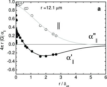
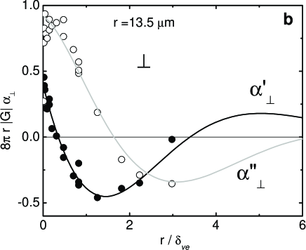
Figure 2: Comparison to Eqs. (8-11) of both real and imaginary parts of the normalized inter-particle response functions between two probe particles (silica beads, $R$ = 0.58 $\mu$m), measured with the active microrheology method for two separation distances $r$ in 1 mg/ml entangled F-actin solutions. (a) $4\pi r|G|\alpha_{||}(\omega)$ and (b) $8\pi r|G|\alpha_{\bot}(\omega)$, plotted versus the ratio of the separation distance $r$ ($r$ = 11.3 $\mu$m in parallel and $r$ = 10.3 $\mu$m in perpendicular direction) to the frequency-dependent viscoelastic penetration depth $\delta_{ve}$. Here, the parameters $\bar{g}$ and $z$ in Eq. (21) were varied to obtain simultaneous fits of all data sets to Eqs. (27-30), using a single set of parameters $z$ and $\bar{g}$, while accounting for the solvent (water) viscosity. Both the real (filled symbols) and imaginary (open symbols) parts of both parallel and perpendicular response functions are in a good agreement with Eqs. (27-30) with optimal parameters $\bar{g}$ = 0.22 $\pm$ 0.05 Pa s^z and $z$ = 0.78 $\pm$ 0.02. The corresponding theoretical lines are shown for $z$ = 0.75 and $\bar{g}$ = 0.22.

The resulting displacement field, exhibiting the vortex pattern, is shown in Fig. 3 for a point force at the origin pointed along the $x$-axis. This flow pattern exhibits specific inversion symmetries: $v_{x}$ ($v_{y}$) is symmetric (antisymmetric) for either $x\rightarrow-x$ or $y\rightarrow-y$, as can be seen by the fact that the (linear) response must everywhere reverse if the direction of the force is reversed.

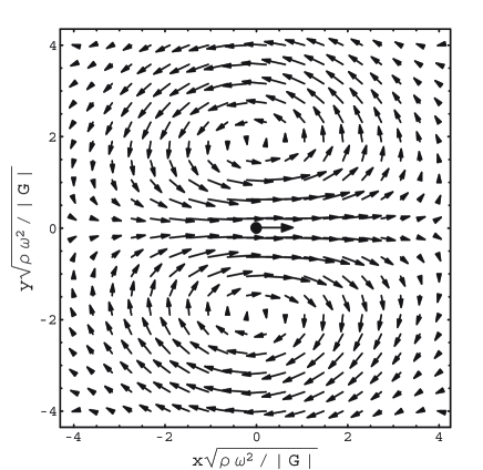
Figure 3: The displacement field displays a clear vortex-like structure. Here, a force in the $\hat{x}$ direction is applied at the origin (as shown by the filled circle and arrow). Distances are shown in units of the penetration depth $\delta=\sqrt{|G|/(\rho\omega^{2})}$. This example has been calculated for the Rouse model with $z=1/2$.

II.2 Velocity autocorrelations and the long time tail

The self-sustaining back-flow represented in Fig. 3 gives rise to long-lived correlations that, for instance, affect the crossover from ballistic to diffusive motion of a particle in a liquid. For a simple liquid, the fluid velocity (auto)correlations $\langle\vec{v}(0,t)\cdot\vec{v}(0,0)\rangle$ decay proportional to $\sim|t|^{-3/2}$. This is known as the long time tail theor_tails ; Alder ; exper_tails . For a viscoelastic fluid, stress propagation is faster than diffusive, resulting in a more rapid decay of velocity correlations. The decay is, however, still algebraic.

II.2.1 Simple liquids

For a simple liquid, Eq. (1) means that

$$\left(-i\omega\rho+\eta k^{2}\right)v_{i}=\left(\delta_{ij}-\hat{k}_{i}\hat{k}_{j}\right)f_{j}$$ (32)

for the Fourier transforms. This gives the response in velocity $v_{i}$ to a force component $f_{j}$ that is (thermodynamically) conjugate to a displacement $u_{j}$. We denote this response function by $\chi_{v_{i}u_{j}}$, where

$$\chi_{v_{i}u_{j}}(\vec{k},\omega)=\frac{\left(\delta_{ij}-\hat{k}_{i}\hat{k}_{j}\right)}{\eta k^{2}-i\omega\rho}.$$ (33)

The fluctuation-dissipation theorem then tells us that

$$\chi_{v_{i}u_{j}}(\vec{r},t)=-\frac{1}{kT}\frac{d}{dt}\langle v_{i}(\vec{r},t)u_{j}(0,0)\rangle,$$ (34)

where this is valid only for $t>0$ because of causality in the response. The correlation function is, however, defined for both positive and negative times.

Due to translation invariance in time, the correlation function $\langle v_{i}(\vec{r},t+t^{\prime})u_{j}(0,t^{\prime})\rangle$ must be independent of $t^{\prime}$. Thus,

$$0 = \frac{d}{dt^{\prime}}\langle v_{i}(\vec{r},t+t^{\prime})u_{j}(0,t^{\prime})\rangle$$

$$= \langle\dot{v}_{i}(\vec{r},t+t^{\prime})u_{j}(0,t^{\prime})\rangle+\langle v_{i}(\vec{r},t+t^{\prime})v_{j}(0,t^{\prime})\rangle,$$

which also means that

$$kT\chi_{v_{i}u_{j}}(\vec{r},t)\rangle\\ =\langle v_{i}(\vec{r},t)v_{j}(0,0)\rangle.$$

Again, this is valid only for $t>0$ because of causality in the response. Ultimately, however, we are interested in the autocorrelation function $\langle\vec{v}\cdot\vec{v}\rangle=\langle v_{i}v_{i}\rangle$, for $r\rightarrow 0$ above. In this case, the correlation function is manifestly symmetric in $t$. Thus,

$$\langle v_{i}(\vec{r}\rightarrow 0,t)v_{i}(0,0)\rangle=kT\chi_{v_{i}u_{i}}(\vec{r}\rightarrow 0,|t|).$$ (36)

We first calculate $\chi_{v_{i}u_{j}}\left(\vec{k},t\right)$, since the limit $\chi_{v_{i}u_{j}}\left(\vec{r}\rightarrow 0,t\right)$ can be obtained from this simply by integrating over all $\vec{k}$.

$$\chi_{v_{i}u_{j}}(\vec{k},t) = \left(\delta_{ij}-\hat{k}_{i}\hat{k}_{j}\right)\int\frac{d\omega}{2\pi}e^{-i\omega t}\frac{1}{\eta k^{2}-i\omega\rho}$$

$$= \frac{\left(\delta_{ij}-\hat{k}_{i}\hat{k}_{j}\right)}{-2\pi i\rho}\int e^{-i\omega t}\frac{d\omega}{\omega+i\nu k^{2}},$$

where $\nu=\eta/\rho$. But, the last integral can only depend on the combination $t\nu k^{2}$, since we can replace $\omega$ by $\zeta\nu k^{2}$, where $\zeta$ is dimensionless. Specifically,

$$\chi_{v_{i}u_{j}}(\vec{k},t) = \frac{\left(\delta_{ij}-\hat{k}_{i}\hat{k}_{j}\right)}{-2\pi i\rho}\int e^{-i\zeta\nu k^{2}t}\frac{d\zeta}{\zeta+i}$$ (37)

$$= \frac{\left(\delta_{ij}-\hat{k}_{i}\hat{k}_{j}\right)}{\rho}e^{-\nu k^{2}t}$$

for $t>0$. Otherwise, the result is zero. This integral can be done by integration along a closed contour containing the real line in either the upper half-plane for $t<0$, or the lower half plane for $t>0$.

Finally, to get the limit

$$\chi_{v_{i}u_{i}}(\vec{r}\rightarrow 0,t)$$ (38)

we simply integrate:

$$\chi_{v_{i}u_{i}}(\vec{r}\rightarrow 0,t) = \int\frac{d^{3}k}{(2\pi)^{3}}\frac{\left(\delta_{ii}-\hat{k}_{i}\hat{k}_{i}\right)}{\rho}e^{-\nu k^{2}t}$$ (39)

$$= \frac{2}{\rho}\left(4\pi\nu t\right)^{-3/2}.$$

Again, this is only for $t>0$. Thus,

$$\langle\vec{v}(\vec{r}\rightarrow 0,t)\cdot\vec{v}(0,0)\rangle=\frac{2kT}{\rho}\left(4\pi\nu|t|\right)^{-3/2}.$$ (40)

II.2.2 Viscoelastic media

For viscoelastic media, the calculation is similar, except that

$$\chi_{v_{i}u_{j}}(\vec{k},\omega) = -i\omega\chi_{u_{i}u_{j}}(\vec{k},\omega)$$ (41)

$$= \chi_{vu}(\vec{k},\omega)\left(\delta_{ij}-\hat{k}_{i}\hat{k}_{j}\right),$$

where $\chi_{u_{i}u_{j}}=\alpha_{ij}$, and where we have defined

$$\chi_{vu}(\vec{k},\omega)=\frac{1}{\rho}\left(\frac{i\omega}{\omega^{2}-G^{*}k^{2}/\rho}\right)$$ (42)

for simplicity. As above, all the singularities in this must lie in the lower half-plane in order for the response function to be causal.

Evaluation of the inverse Fourier transform of Eq. (42) to obtain $\chi_{vu}(\vec{k},t)$ can be done by use of the Mittag-Leffler functions. The Mittag-Leffler functions podlubny ; erdelyi , $E_{\alpha}(z)$, which are entire functions parameterized by a continuous parameter $\alpha$ can be defined by the power series

$$E_{\alpha}(z)=\sum_{k=0}^{\infty}{z^{k}\over\Gamma(1+\alpha k)}\quad;\quad\alpha>0\quad.$$ (43)

Note $E_{1}(x)=\exp(x)$. Straightforward manipulation podlubny of the definition, Eq. (43) show that their causal Fourier transforms are given by

$$\int_{-\infty}^{\infty}dte^{i\omega t}\Theta(t)E_{\alpha}(-at^{\alpha})={i\omega\over\omega^{2}-a\left(-i\omega\right)^{2-\alpha}}$$ (44)

where $\Theta(t)$ is the Heaviside step function. Performing the inverse Fourier transform, we obtain

$$\chi_{vu}(\vec{k},t)=E_{2-z}\left[-(\bar{g}k^{2}/\rho)t^{2-z}\right]\quad;\quad t>0$$ (45)

for $G^{*}=\bar{g}(-i\omega)^{z}$. The asymptotic expansions for the Mittag-Leffler functions podlubny ; paris are

$$E_{\alpha}(-z)=\left\{\begin{array}[]{c}\displaystyle 1-{z\over\Gamma(1+\alpha)}+O(z^{2})\,,\quad z\ll 1\\ \displaystyle{z^{-1}\over\Gamma(1-\alpha)}+O(z^{-2})\,,\quad z\gg 1\end{array}\right.$$ (46)

Thus, the velocity correlation function is given by

$$\langle\vec{v}(\vec{r}\rightarrow 0,t)\cdot\vec{v}(0,0)\rangle=$$ (47)

$$\frac{2kT}{\rho}{4\pi\over(2\pi)^{3}}\int_{0}^{1/a} \!\!\!\!\!\!\!\!\!k^{2}dkE_{2-z}\left[-(\bar{g}k^{2}/\rho)|t|^{2-z}\right]$$

From the asymptotic properties of $E_{\alpha}(t)$, it is clear that the integral does not converge at $k\rightarrow\infty$ necessitating a finite cut-off (which we choose as the size of the probe particle). We can express the correlation function as

$$\langle\vec{v}(0,t)\cdot\vec{v}(0,0)\rangle = |t|^{-\frac{3}{2}{(2-z)}}\frac{2kT}{\rho}\left({\rho\over\bar{g}}\right)^{3/2}{2-z\over(2\pi)^{2}}I_{2-z}$$

$$I_{\alpha} = \int_{0}^{\Lambda_{\alpha}}dxx^{3\alpha/2-1}E_{\alpha}\left(-x^{\alpha}\right)$$ (48)

and $\Lambda_{\alpha}=(|t|\bar{g}/\rho a^{2})^{1/\alpha}$.

We can get an approximation to the value of $I_{\alpha}$ by splitting the integral into two sections

$$I_{\alpha}=\int_{0}^{1}dxE_{\alpha}^{\ll}(-x^{\alpha})+\int_{1}^{\Lambda_{\alpha}}dxE_{\alpha}^{\gg}(-x^{\alpha})$$

using the two asymptotic forms for $E_{\alpha}(t)$.

We then obtain finally the expression

$$\langle\vec{v}(\vec{r}\rightarrow 0,t)\cdot\vec{v}(0,0)\rangle\simeq C_{1}|t|^{-3(2-z)/2}+C_{2}|t|^{-(5-3z)/2}$$ (49)

where

$$C_{1} =\frac{4kT}{(2\pi)^{2}\rho}\left({\rho\over\bar{g}}\right)^{3/2}\times$$

$$\frac{5\Gamma(3-z)\Gamma(z-1)-3\Gamma(z-1)-15\Gamma(3-z)}{15\Gamma(3-z)\Gamma(z-1)}$$

and

$$C_{2}=\frac{4kT}{(2\pi)^{2}a\rho}\left({\rho\over\bar{g}}\right){1\over\Gamma(z-1)}.$$ (51)

Here, the dominant first term in Eq. (49) corresponds to a faster asymptotic decay of correlations for $z<1$ than for simple liquids. This is a direct consequence of the super-diffusive propagation of stress in this case. Also, it is interesting to note that the second term in Eq. (49) strictly vanishes in the $z\rightarrow 1$ limit of simple liquids.

III MATERIALS AND METHODS

Simple liquids: For our experiments we used two Newtonian fluids with different viscosities $\eta$ and mass densities $\rho$, namely water ($\eta$ = 0.969 mPas and $\rho$ = 1000 kg$m^{-3}$) and a $(1:1~{}v/v)$ water/glycerol mixture ($\eta$ = 6.9 mPas and $\rho$ = 1150 kg$m^{-3}$).

Viscoelastic fluids: We performed experiments with two different viscoelastic fluids, worm-like micelle solutions and solutions of the cytoskeletal biopolymer F-actin. Worm-like micelles were prepared by self-assembly of cetylpyridinium chloride (CPyCl) in brine (0.5M NaCl) with sodium salicylate (NaSal) as counterions, with a molar ratio of Sal/CPy = 0.5. Three different concentrations of worm-like micelles were used: $c_{m}$ = 0.5%,1% and 2%. Worm-like micelles behave essentially like linear flexible polymers with an average diameter of about 3 nm, a persistence length of about 10 nm, and contour lengths of several $\mu$m Berret . F-actin was polymerized from monomeric actin (G-actin) isolated from rabbit skeletal muscle according to a standard recipe  Pardee . G-actin was mixed with silica beads in polymerization buffer [2 mM HEPES, 2 mM MgCl₂, 50 mM KCl, 1 mM Na₂ATPa, and 1 mM EGTA, pH 7] and incubated for 1 hour. Entangled actin solutions were used as a model system for semiflexible polymer solutions. Experiments were done at concentrations of c = 0.5 and 1 mg/ml.

III.1 Experimental methods

Details of the experimental set-up can be found in Allersma ; setup maryam ; Mizuno active ; MizunoTechnical . Briefly, we have used a custom-built inverted microscope that includes a pair of optical traps formed by two focused laser beams of different wavelengths ($\lambda$ = 1064 nm, ND:YVO₄, Compass, Coherent, Santa Clara, CA, USA) and $\lambda$ = 830 nm (diode laser, CW, IQ1C140, Laser 2000). The optical traps fulfil two functions: (i) They confine the particles around two well-defined positions and at the same time detect particle displacements with high temporal and spatial resolution in the passive method. (ii) In the active method one trap is used to apply a sinusoidally varying force to one particle, while the response of the other particle is detected in the second trap. In the passive method, a pair of silica beads (Van’t Hoff Laboratory, Utrecht University, Utrecht, Netherlands) of various radii (R = 0.25  $\mu$m $\pm$5%, 0.580 $\mu$m $\pm$5%, 1.28$\mu$m $\pm$5% and 2.5 $\mu$m$\pm$5%) were weakly trapped (trap stiffness between 2 $\mu$N/m and 5 $\mu$N/m, where larger particles required the higher laser intensities to avoid shot noise. Transmitted laser light was imaged onto two quadrant photo diodes, such that particle displacements and in the $x$ and $y$ directions were detected interferometrically detection Gittes . A specialized silicon PIN photodiode (YAG444-4A, Perkin Elmer, Vaudreuil, Canada), operated at a reverse bias of 110 V, was used in order to extend the frequency range up to 100 kHz for the 1064 nm laser Erwin detection . The 830 nm laser was detected by a standard silicon PIN photodiode operated at a reverse bias of 15 V (Spot9-DMI, UDT, Hawthorne, CA). Amplified outputs were digitized at 195 kHz (A/D interface specs ) and further processed in Labview (National Instruments, Austin, TX, USA). Output voltages were converted to actual displacements using Lorentzian fits to power spectral densities (PSD) as described in signal and noise . In the case of water, calibration was done on the beads that were used in the experiments, while for the viscoelastic solutions and the more viscous liquid, calibrations were done in water with beads from the same batch.

In the active method, the 1064 nm laser was used to oscillate one particle, while the 830 nm laser was used for detection of the second particle at a separation distance $r$. The driving laser was deflected through an Acousto-Optical Deflector (AOD) (TeO₂, Model DTD 276HB6, IntraAction, Bellwood, Illinois), using a voltage-controlled oscillator (VCO) (DRF.40, AA OPTO-ELECTRONIC, Orsay, France). The force applied to the driven particle was calibrated by measuring the PSD of the Brownian motion of a particle of the same size trapped in water with the same laser power signal and noise . The output signal from the QPD detecting the second laser was fed into a lock-in amplifier (SR830, Stanford Research Systems, Sunnyvale, CA, USA) to obtain amplitude and phase of particle response. All experiments were done in sample chambers made from a glass slide and a cover slip with about 140 $\mu$m inner height, with the particles at at least 25 $\mu$m distance from both surfaces. The lab temperature was stabilized at T = $21.5~{}^{\circ}$C.

IV DATA ANALYSIS

In both the active and passive methods we calculate the linear complex response function $\alpha$ defined by $u(\omega)=\alpha(\omega)\times F(\omega)$, where $F(\omega)$ is the applied force. Linear response applies by definition in the passive method, and in the active method the particle displacements $u(\omega)$ were kept sufficiently small. Again, we consider separately real, $\alpha^{\prime}(\omega)$, and imaginary parts, $\alpha^{\prime\prime}(\omega)$, of the response. In all our experiments, as sketched in Fig. 4, the coordinate system was chosen in such a way that $x$ is parallel to the line connecting the centers of the two particles ($||$) and $y$ perpendicular ($\bot$)to that. The inter-particle response functions along these two directions were used to determine the flow field.

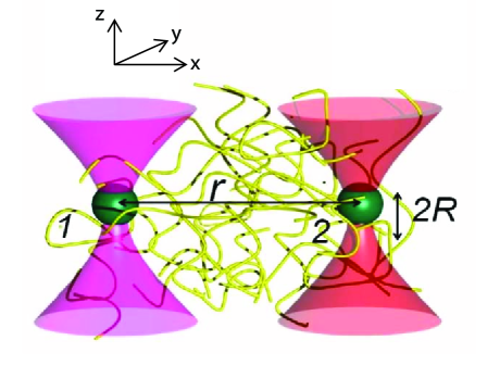
Figure 4: (Color online) Schematic sketch of the experiment. A pair of silica beads (radius $R$) is trapped by a pair of laser traps at a separation distance $r$. In the passive method, the position fluctuations of each particle in the $x$ and $y$ directions are simultaneously detected with quadrant photodiodes and the displacement cross-correlations are measured parallel and perpendicular to the line connecting the centers of the two beads. In the active method, one of the beads is oscillated by rapidly moving one laser trap either in $x$ or in $y$ direction and the resulting motion of the other particle is measured in $x$ and in $y$ direction. Laser intensity was adjusted to result in the trap stiffness of typically between (2$\mu N/m$ and 5$\mu N/m$) for passive measurements.

The displacement $u^{(1)}_{x}(\omega)$ of particle 1 in the $x$ direction is related to the force $F^{(2)}_{x}$ acting on particle 2 according to $u^{(1)}_{x}(\omega)=\alpha_{||}(\omega)\times F^{(2)}_{x}(\omega)$. Similarly, the perpendicular response function was derived from $u^{(1)}_{y}(\omega)=\alpha_{\bot}(\omega)\times F^{(2)}_{y}(\omega)$. The single-particle response functions for each $x$ and $y$ directions are defined as $u^{(1)}_{x,y}(\omega)=\alpha_{\rm auto}(\omega)\times F^{(1)}_{x}(\omega)$. For homogeneous, isotropic media, the two functions $\alpha_{||,\bot}(\omega)$ completely characterize the linear response at any point in the medium due to a force at another point. The displacement response functions $\alpha_{||,\bot}(\omega)$ determine both position and velocity response $-i\omega\alpha_{||,\bot}(\omega)$.

In the passive approach, the medium fluctuates in equilibrium, and the only forces on the particles are thermal/Brownian forces. Therefore the fluctuation-dissipation theorem (FDT) of statistical mechanics Landau stat relates the response of the medium to the displacement correlation functions. For two particles, these correlation functions are the cross-correlated displacement fluctuations: $\langle u^{(1)}_{x}(t)u^{(2)}_{x}(0)\rangle$ and $\langle u^{(1)}_{y}(t)u^{(2)}_{y}(0)\rangle$. We used Fast Fourier Transforms (FFT) to calculate displacement cross-correlation functions in frequency space and obtained the imaginary parts of the complex inter-particle response functions $\alpha^{\prime\prime}_{||,\bot}(\omega)$ via the FDT:

$$\alpha^{\prime\prime}_{||}(\omega)=\frac{\omega\int\langle u^{(1)}_{x}(t)u^{(2)}_{x}(0)\rangle e^{i\omega t}dt}{2kT}$$ (52)

and

$$\alpha^{\prime\prime}_{\bot}(\omega)=\frac{\omega\int\langle u^{(1)}_{y}(t)u^{(2)}_{y}(0)\rangle e^{i\omega t}dt}{2kT},$$ (53)

where k is the Boltzman constant and T is the controlled laboratory temperature. The real parts of inter-particle response functions $\alpha^{\prime}_{||,\bot}(\omega)$ were obtained by a Kramers-Kronig integral:

$$\alpha^{\prime}_{||,\bot}(\omega) = \frac{2}{\pi}P\int^{\infty}_{0}\frac{\zeta\alpha^{\prime\prime}_{||,\bot}(\omega)}{\zeta^{2}-\omega^{2}}$$

$$= \frac{2}{\pi}\int^{\infty}_{0}\cos(t\omega)\int^{\infty}_{0}\alpha^{\prime\prime}_{||,\bot}(\zeta)\sin(t\zeta)d\zeta,$$

where P denotes a principal-value integral MR97 . The high frequency cut-off of the Kramers-Kroning integral limits the frequency range of the calculated $\alpha^{\prime}_{||,\bot}(\omega)$ setup maryam . We also used the active method to obtain both real and imaginary parts of the response functions with 100 kHz bandwidth, as in Refs. Mizuno active ; MizunoTechnical . Here the lock-in amplifier provides directly in-phase (real part) and out-of-phase (imaginary part) response of the second particle. The measurements were done over a grid of driving frequencies.

V RESULTS

V.1 Simple liquids

In the low-frequency limit, where fluid inertia can be neglected, the inter-particle response functions are inversely related to the shear modulus of the medium Mason ; MR97 ; 2fluid . For a simple viscous fluid, the response functions in this limit are given by:

$$\alpha_{||}=2\alpha_{\perp}=\frac{i}{4\pi r\omega\eta}$$ (55)

where $r$ is the separation distance between the two particles and $\eta$ is the viscosity. These relations also shows (via the FDT) a $1/r$ dependence of the Fourier transform of the displacement cross-correlation functions:

$$S_{||}=\int\langle u^{(1)}_{x}(t)u^{(2)}_{x}(0)\rangle e^{i\omega t}dt$$ (56)

and

$$S_{\perp}=\int\langle u^{(1)}_{y}(t)u^{(2)}_{y}(0)\rangle e^{i\omega t}dt$$ (57)

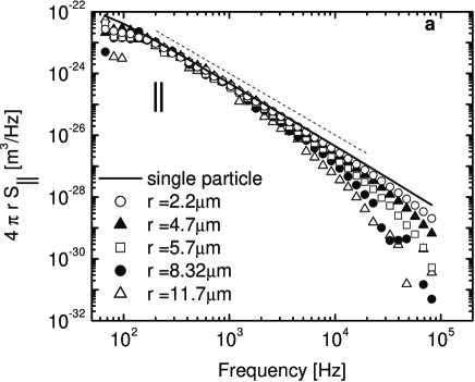
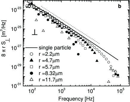
Figure 5: Normalized displacement cross-correlation functions (a) $4\pi rS_{||}$ and (b) $8\pi rS_{\bot}$ of two probe particles (silica beads, $R$ = 0.58 $\mu$m) in water versus frequency ($f=\omega/2\pi$), compared for different separation distances $r$ (symbols). In both (a) and (b), the solid line is the auto-correlation function of a single particle, normalized by $6\pi R$. The single-particle motion agrees well with the expected frequency dependence of a single Brownian particle (slope of -2), as indicated by the dashed lines.

In Fig. 5, displacement cross-correlation functions for particle pairs in water, normalized to compensate for the distance dependence ($4\pi rS_{||}$ and $8\pi rS_{\bot}$ ), are plotted versus frequency. For comparison a single-particle displacement auto-correlation function, normalized for the bead size dependence ($6\pi RS_{\rm auto}$), is plotted as a solid line, for a particle radius of $R=0.58~{}\mu m$. The auto-correlation function agrees well with the power-law slope of -2 up to nearly 100 kHz. This slope is expected from the high-frequency limit of the Lorentzian shape of the power spectral density (= Fourier Transform of the displacement autocorrelation function) of the displacements of a harmonically confined Brownian particle in a viscous fluid signal and noise . The effect of fluid inertia is evident as a deviation from this power law in the displacement cross-correlation functions. A systematically $r$ dependent decrease of the cross-correlations is apparent at high frequencies for separations r ranging from $2.2~{}\mu m$ to $11.7~{}\mu m$. The faster decrease of cross-correlations is a manifestation of the finite velocity at which stress propagates into the medium. For larger $r$, the data show that the decrease begins at a lower frequency, because it takes longer for stress to propagate further. A comparison of Figs. 5a and b shows that the decrease of the cross-correlation is, at the same separation distance, more pronounced in the perpendicular channel than in the parallel channel. This is due to the fact that in the vortex-like flow pattern of Fig. 3 there is a region of fluid motion in the opposite direction to the applied force. For $r>5~{}\mu m$ (open squares), the cross-correlations become negative in the observed frequency window (not shown in the log-log plot). At still higher frequencies, the displacement cross-correlation functions again become positive (Fig. 5b), which is visible for the larger separations, $r=8.3~{}\mu m$ and $r=11.7~{}\mu m$, consistent with the expected oscillation in the displacement cross-correlation functions in the frequency domain. This effect becomes more pronounced in viscoelastic media

The spatial and temporal propagation of the inertial vortex in a general viscoelastic medium is characterized by Eqs. (8-11) Oseen ; maryam ; liverpool . For simple liquids, A = $\eta$ (viscosity) and z = 1. In Figs. 6a and b, we compare the imaginary parts of the normalized inter-particle response functions $4\pi\eta r\omega\alpha^{\prime\prime}_{||}(\omega)$ (Fig. 6a) and $8\pi\eta r\omega\alpha^{\prime\prime}_{\bot}(\omega)$ (Fig. 6b) for water and a (1:1 v/v) water/glycerol mixture. In order to collapse all data onto a single master curve, as suggested by Eqs. (8-11), we have plotted these normalized response functions versus the probe particle separation r scaled by the corresponding frequency-dependent penetration depth $\delta_{v}=\sqrt{\eta/\rho\omega}$. As shown in Fig. 6, data taken at all of the different separations $r$ ranging from $2.2~{}\mu m$ to $11.7~{}\mu m$ fall onto a single curve for both, the parallel (Fig. 6a) and the perpendicular (Fig. 6b) inter-particle response functions. Data for water also collapse on water/glycerol data, after accounting for the different viscosities, which are known in both cases. Thus, no free fit parameters were used. The single curves of collapsed data are in quantitative agreement with the frequency-dependent dynamic Oseen tensor in Eqs. (12,13) shown by the solid lines in Figs. 6a and b, where the region of negative response in the perpendicular direction corresponds again to the back-flow region of the vortex already described above.

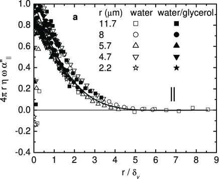
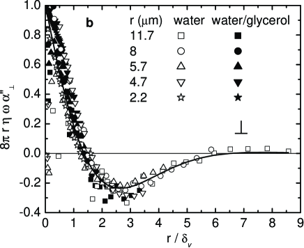
Figure 6: Normalized imaginary parts of inter-particle response functions between two probe particles (silica beads, $R$ = 0.58 $\mu$m) measured with the passive method, (a) $4\pi r\eta\omega\alpha^{\prime\prime}_{||}$ in the parallel direction and (b) $8\pi r\eta\omega\alpha^{\prime\prime}_{\bot}$ in the perpendicular direction, plotted versus the ratio of the separation distance $r$ (fixed for a given bead pair) to the frequency-dependent viscous penetration depth $\delta_{v}$, in water (open symbols, $\eta$ = 0.969 mPa s) and in water/glycerol (filled symbols, $\eta$ = 6.9 mPa s). Solid lines are Oseen’s predictions for a simple liquid with no adjustable parameters. Data is only plotted for $\omega>$ 200 rad/s and for $\omega<$ 2krad/s one in every 5 data points is shown.

At separations $r$ large compared to particle size, the inter-particle response functions become independent of probe particle size and shape 2fluid , leaving a dependence only on $r$ and $\omega$. In our analysis, we have assumed that the particles are point-like since the ratio $r/R\geq 4$ in all experiments. In order to directly check the validity of the approximation, we measured the inter-particle response functions with particles of different sizes. In Fig. 7a and b the imaginary parts of the normalized response functions in water $4\pi\eta r\omega\alpha^{\prime\prime}_{||}(\omega)$ and $8\pi\eta r\omega\alpha^{\prime\prime}_{\bot}(\omega)$ are plotted versus $r/\delta_{v}$, obtained with probe particles of radius $R$ = 0.58$~{}\mu m$, 1.05 $\mu m$, 1.28 $\mu m$ and 2.5 $\mu m$. We find no systematic bead-size dependence, justifying the point-probe approximation. Again all normalized and scaled data collapse onto one single curve for each channel, which in turn agrees well with the dynamic Oseen tensor. The deviations observed in the last data points for $R$ = 1.05 $\mu m$ and 2.5 $\mu m$ are most probably due to the influence of shot noise at high frequencies. Shot noise becomes a problem for larger beads because of their smaller fluctuation amplitudes, which will eventually produce signals that approach the fixed shot noise level. The deviations observed for these particle sizes are not consistent with a possible error due to finite particle size, which should be larger for smaller $r/R$.

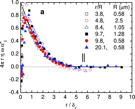
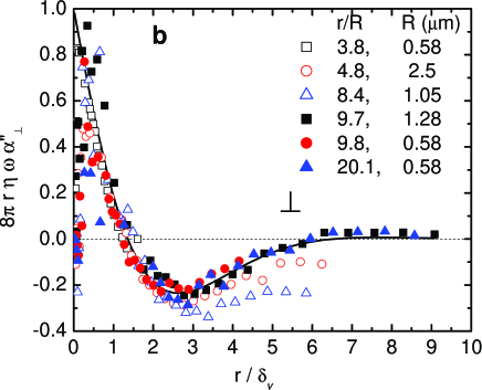
Figure 7: (Color online) Normalized imaginary parts of inter-particle displacement response functions between two probe particles of various radii measured with the passive method in water (silica beads, $R$ given in legend),(a) $4\pi r\eta\omega\alpha^{\prime\prime}_{||}$ in the parallel direction and (b) $8\pi r\eta\omega\alpha^{\prime\prime}_{\bot}$ in the perpendicular direction, plotted versus the ratio of the separation distance $r$ (fixed for a given bead pair) to the frequency-dependent viscous penetration depth $\delta_{v}$. These response functions also represent the in-phase velocity response normalized by the corresponding components of the Oseen tensor. Different particle sizes (R = 0.58, 1.05, 1.28 and 2.5 $\mu$m) were used at various separation distances $r$.

So far, we have considered the passive fluctuations that directly measure only the imaginary (out-of phase) part of the inter-particle response functions ($\alpha^{\prime\prime}_{||,\bot}(\omega)$). With the active method described in Sec. III.1 we can determine both real and imaginary part of the response functions. In Figs. 1a and b, we show the normalized inter-particle response functions $\alpha^{\prime}_{||,\bot}(\omega)$ and $\alpha^{\prime\prime}_{||,\bot}(\omega)$ measured by active microrheology (bead radius $R$= 0.58 $\mu m$) in water for both parallel and perpendicular direction. In both cases we find good agreement with Eqs. (12,13). The slightly different separation distances in parallel ($r$ = 10.3 $\mu m$) and perpendicular ($r$ = 11.3 $\mu m$) were due to different settings of the AOD signal in these measurements.

V.2 Viscoelastic solutions

In viscoelastic polymer solutions, the elastic component in the response of the medium modifies the propagation of the inertial vortex. We first discuss our results for worm-like micelle solutions, the viscoelastic properties of which have been characterized by microrheology micelles ; Atakhorrami micelles . In Fig. 8 we have plotted the displacement cross-correlation functions ($4\pi rS_{||}$ and $8\pi rS_{\bot}$) in a 1% worm-like micelle solution versus frequency for two particles at various separation distances $r$ between 2 and $8~{}\mu m$. For comparison, we have added the scaled auto-correlation function $6\pi RS_{auto}$ for a single particle ($R$ = 0.58 $\mu m$). In contrast to the situation in simple liquids, the particles were here confined by the surrounding polymer network and do not diffuse freely. Thus, the frequency dependence is weaker than for Brownian motion (i.e., the slope is less steep than -2 in the low-frequency, non-inertial regime) micelles ; Atakhorrami micelles . As before, the displacement cross-correlation functions of the two probe particles are used to map the vortex-like flow pattern and its propagation in time. The $r$-dependent decrease of the cross-correlation functions occurs for both parallel (Fig. 8a) and perpendicular (Fig. 8b) directions, although the latter is more apparent.

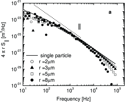
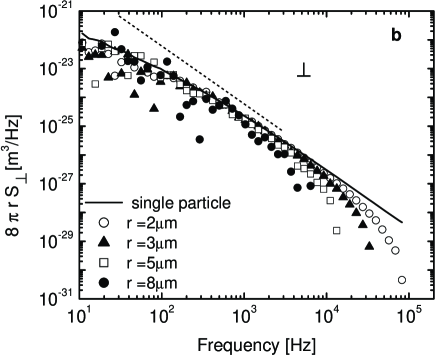
Figure 8: Normalized displacement cross-correlation functions $4\pi rS_{||}$ (a) and $8\pi rS_{\bot}$ (b) of two probe particles (silica beads, $R$ = 0.58 $\mu$m) in worm-like micelle solutions (c_m = 1 wt%) versus frequency ($f=\omega/2\pi$) compared for different separation distances $r$. The solid lines represent the auto-correlation function of a single particle normalized by $6\pi R$. The dashed lines indicate slopes of -2, corresponding to diffusive motion.

In order to collapse these data onto a single curve for each of the two channels (parallel and perpendicular), following Eqs. (8-11), we plot the normalized inter-particle response functions $4\pi|G|r\alpha^{\prime\prime}_{||}$ and $8\pi|G|r\alpha^{\prime\prime}_{\bot}$ versus scaled $r/\delta_{ve}$ , where $\delta_{ve}$ is the viscoelastic penetration depth. Unlike for the water and water/glycerol samples, we do not a priori know the frequency-dependent shear modulus $G^{\star}(\omega)$. Based on theoretical expectations for flexible polymers Doi , as well as on prior high-frequency rheology of worm-like micelle solutions micelles ; Atakhorrami micelles , we assume that the shear modulus has the functional form given in Eq. (21). Thus, in order to achieve the collapse of all data onto the master curves represented by Eqs. (8-11), we vary the two correlated parameters $\bar{g}$ and $z$. We expect $z$ to be independent of the micelle concentration, while $\bar{g}$ should depend linearly on the polymer/micelle concentration. In Fig. 9a, we show the resulting collapse of the normalized inter-particle response functions in parallel and perpendicular directions for different separations $r$. The predictions of Eqs. (8-11) are shown with black and gray lines liverpool . The best overall collapse of the data for worm-like micelles solutions at all concentrations (0.5, 1 and 2 weight percent) and separations $r$ from $2~{}\mu m$ to $16~{}\mu m$ was found for $z$ = 0.68 $\pm$ 0.05 and $\bar{g}$ concentration dependence as seen in Fig. 9b.

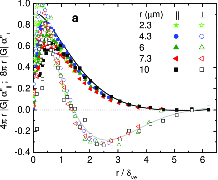
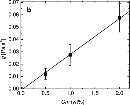
Figure 9: (Color online) (a) Collapse of the imaginary parts of the normalized inter-particle response functions ($4\pi r|G|\alpha^{\prime\prime}_{||}(\omega)$ and $8\pi r|G|\alpha^{\prime\prime}_{\bot}(\omega)$) between two probe particles (silica beads, $R$ = 0.58 $\mu$m), measured with the passive method for different separation distances $r$ in worm-like micelle solutions of 1 wt%, plotted versus the ratio of the separation distance $r$ (fixed for a given bead pair) to the frequency-dependent viscoelastic penetration depth $\delta_{ve}$. Here, the viscoelastic penetration depths were determined by varying the parameters $\bar{g}$ and $z$ in Eqs. (8-11,21) to obtain collapse. Optimal parameters were $z$ = 0.68 $\pm$ 0.05 and $\bar{g}$ = 0.0275 $\pm$ 0.008 Pa s^z, where the solvent (water) viscosity has been taken into account. (b) Dependence of (optimal) parameter $\bar{g}$ on micelle concentration for a fixed $z$.

In order to further test the inertial effects in viscoelastic media, we also performed experiments on another viscoelastic fluid with a somewhat different frequency dependent shear modulus, namely entangled F-actin solutions. At high frequency, semiflexible F-actin filaments contribute to the viscoelasticity of the medium in a different way from flexible polymers Morse98 ; Gittes98 ; MR97 ; Koenderink actin . Therefore, the spatial structure and the propagation dynamics of the vortex should be different. Figure 10 shows the collapse of the inter-particle response functions $4\pi|G|r\alpha^{\prime\prime}_{||}$ and $8\pi|G|r\alpha^{\prime\prime}_{\bot}$ plotted versus scaled distance $r/\delta_{ve}$ onto two master curves for the parallel and the perpendicular direction. The actin concentration was 1mg/ml and the probe radius 0.58 $\mu m$ and we used separation distances $r$ ranging from 4.2 $\mu m$ to 16.2 $\mu m$. In an F-actin solution of this concentration, the magnitude of the shear modulus is large, therefore the vortex propagates faster, making it harder to observe. In particular, it was difficult to determine the parameters $\bar{g}$ and $z$ in this case. We found the best collapse with $z$ = 0.78 $\pm$ 0.1 for data taken in passive method. We then fixed $z$ to 0.75 known from the power law dependence behavior reported previously Morse98 ; Gittes98 ; MR97 ; Koenderink actin , and found $\bar{g}$ = 0.18 $\pm$ 0.13Pa s^z. To reduce the large error bars in the passive method, it would be necessary to repeat our measurements at higher frequencies and/or larger separation distances. Nevertheless, our results are consistent with prior measurements and predictions of both parameters.

Independently, we have measured both real, $\alpha^{\prime}_{||,\bot}(\omega)$, and imaginary, $\alpha^{\prime\prime}_{||,\bot}(\omega)$, parts of the response functions directly by actively manipulating one particle and measuring the response of the other. In Figs. 2a and b, the parallel (Fig. 2a) and perpendicular (Fig. 2b) complex inter-particle response functions for $c$ = 1 mg/ml F-actin solutions are shown, probed with beads of 1.28 $\mu m$ radius. Here the inter-particle response functions were fitted with Eqs. (8-11) to find parameters $\bar{g}$ = 0.22$\pm$0.05 Pa s^z and $z$= 0.78$\pm$0.01 simultaneously. Data for both parallel ($r$ = 12.1 $\mu m$) and perpendicular ($r$ = 13.5 $\mu m$) channels are compared with $z$ = 0.75 and $\bar{g}$ = 0.22 Pa s^z in Fig. 2a and b.

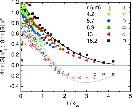
Figure 10: (Color online) Collapse of the imaginary parts of the normalized inter-particle response functions between two probe particles (silica beads, $R$ = 0.58 $\mu$m), measured with the passive method for different separation distances $r$ in F-actin solutions of concentration 1 mg/ml, plotted versus the ratio of the separation distance $r$ (fixed for a given bead pair) to the frequency-dependent viscoelastic penetration depth $\delta_{ve}$. Here, the parameters $\bar{g}$ and $z$ in Eq. (21) were varied to obtain simultaneous collapse of all data sets onto Eqs. (8-11), using a single set of parameters $z$ and $\bar{g}$, while accounting for the solvent (water) viscosity. We find $z$ = 0.78 $\pm$ 0.1, and $\bar{g}$ = 0.18 $\pm$ 0.13 as optimal parameters. Data are presented for parallel (closed symbols) and perpendicular (open symbols) directions. The solid black line represents Eq. (28) and the gray line represents Eq. (30), both with $z$ = 0.75 and $\bar{g}$ = 0.2 Pa s^z.

The values of $z$ and $\bar{g}$ found from both methods are consistent and also agree with results from prior experimental microrhelogy and macrorheology experiments for both entangled actin solutions MR97 ; Morse98 ; Gittes98 ; Gardel ; Koenderink actin and worm-like-micelle solutions micelles ; Atakhorrami micelles . To obtain these values it was essential to model the inertial effects including both polymer and solvent contributions to the shear modulus. We observed that, although the high-frequency rheology of the polymer solution is dominated by the polymer, the background solvent contributes non-negligibly to the inertial vortex propagation. To test this, we excluded the solvent shear modulus ($-i\omega\eta$) in Eqs. (8-11,21), and analyzed our data assuming a high-frequency shear modulus of the form $G=\bar{g}\omega^{z}$. For both worm-like micelle solutions and entangled F-actin solutions, we found much larger values of $z\sim$ 0.9 and a nonlinear concentration dependence of $\bar{g}$, contrary to expectations.

VI DISCUSSION

In our experiments we have directly resolved the inertial response/flow of fluids on micrometer and microsecond time scales using optical trapping and interferometric particle-tracking. Our results demonstrate that vorticity and stress propagate diffusively in simple liquids and super-diffusively in viscoelastic media. One consequence of inertial vortex formation is the long-time tail effect observed in light scattering experiments exper_tails . To connect to these results, we calculated the velocity auto-correlation of a single particle from the displacement fluctuations. Unfortunately, the effect we are looking for is subtle and is difficult to detect in the presence of other factors. At the highest frequencies the vortex is still influenced by the finite probe size, and at intermediate frequencies the particle motion is already affected by the laser trap potential. The results were thus inconclusive. Similar problems have been reported in Ref. Lukic . The effects of inertia we have described here set a fundamental limit to the applicability of two-particle microrheology techniques which are based on the measurement of cross-correlated position fluctuations of particles crocker ; Gardel ; 2fluid ; micelles ; Koenderink actin . Inertia limits the range of stress propagation at high frequencies, stronger in soft media such as those studied here than in media with higher viscoelastic moduli. Inertia affects measurements at frequencies as low as 1 kHz for separations of order 10 micrometers, showing an apparent increase of the measured shear moduli below their actual values Atakhorrami micelles . Since the stress propagation is diffusive, or nearly so, even measurements at video rates can be affected for probe particle separations of order 50 micrometers. As we have shown here, these inertial effects are more pronounced in the perpendicular inter-particle response functions than in the parallel ones. This suggests that one should obtain shear moduli from the parallel inter-particle response functions if one doesn’t want to correct for inertia. In a more precise analysis of two-particle microrheology experiments, the fluid response function can not simply be modeled by a generalized Stokes-Einstein relationship and has to be corrected for inertial effects according to the probed frequency as well as the particles separation. Such corrections, however, will necessarily be limited, given the exponential attenuation of stress due to inertia.

VII Acknowledgments

Actin was purified by K.C. Vermeulen and silica particles were kindly donated by C. van Kats (Utrecht University). F. Gittes, J. Kwiecinska, and J. van Mameren helped with developing the data analysis software. We thank D. Frenkel, W. van Saarloos, A.J. Levine and K.M. Addas for helpful discussions. This work was supported by the Foundation for Fundamental Research on Matter (FOM). Further support (C.F.S.) came from the DFG Center for the Molecular Physiology of the Brain (CMPB) and the DFG Sonderforschungsbereich 755.

References

- (1) L.D. Landau and E.M. Lifshitz, Fluid Mechanics, Butterworth-Heinemann (Oxford, 2000).
- (2) J. Happel and H. Brenner, Low Reynolds Number Hydrodynamics, McGraw-Hill (New York, 1963)
- (3) E. Guyon et al, Physical Hydrodynamics, Oxford University Press (New York, 2001)
- (4) C.W. Oseen, Hydrodynamik (Akademische Verlagsgesellschaft, Leipzig, 1927), p. 47.
- (5) B.J. Alder and T.E. Wainwright, Phys. Rev. A 1, 18 (1970).
- (6) J.P. Boon and A. Bouiller, Phys. Lett. 55A, 391 (1967); G.L. Paul and P.N. Pusey, J. Phys. A 14, 3301 (1981); K. Ohbayashi, T. Kohno, and H. Utiyama, Phys. Rev. A 27, 2632 (1983); D.A. Weitz, D.J. Pine, P.N. Pusey, and R.J.A. Tough, Phys. Rev. Lett. 63, 1747 (1989).
- (7) M. Atakhorrami, G.H. Koenderink, C.F. Schmidt, and F.C. MacKintosh, Phys. Rev. Lett. 95, 208302 (2005).
- (8) R. Zwanzig and M. Bixon, Phys. Rev. A 2, 2005 (1970); M.H. Ernst, E.H. Hauge, and J.M.J. van Leeuwen, Phys. Rev. Lett. 25, 1254 (1970); J.R. Dorfman and E.G.D. Cohen, Phys. Rev. Lett. 25, 1257 (1970); D. Bedeaux and P. Mazur, Phys. Lett. 43A, 401 (1973); D. Bedeaux and P. Mazur, Physica (Amsterdam) 73, 431 (1974).
- (9) B. Lukic, S. Jeney, C. Tischer, et al., Phys. Rev. Lett. 95, 160601 (2005).
- (10) C. Morkel, C. Gronemeyer, W. Glaser, J. Bosse, Phys. Rev. Lett. 58, 1873 (1987).
- (11) T.B. Liverpool and F.C. MacKintosh, Phys. Rev. Lett. 95, 208303 (2005).
- (12) F. Gittes and C.F. Schmidt, Optics Lett. 23, 7 (1998).
- (13) M. Atakhorrami, K.M. Addas and C.F. Schmidt, unpublished.
- (14) J.C. Crocker, M.T. Valentine, E.R. Weeks, T. Gisler, P.D. Kaplan, A.G. Yodh, and D.A. Weitz, Phys. Rev. Lett. 85, 888 (2000).
- (15) J-C. Meiners and S.R. Quake, Phys. Rev. Lett. 82, 2211 (1999).
- (16) S. Henderson, S. Mitchell, and P. Bartlett, Phys. Rev. E 64, 061403 (2001)
- (17) L. Starrs and P. Bartlett, Journal of Physics-Cond. Mat. 15, S251 (2003).
- (18) M.L. Gardel, M.T. Valentine, J.C. Crocker, A.R. Bausch and D.A. Weitz, Phys. Rev. Lett. 91, 158302 (2003).
- (19) G.H. Koenderink, M. Atakhorrami, F.C. MacKintosh, C.F. Schmidt, Phys. Rev. Lett. 96:138307 (2006).
- (20) F. Gittes, B. Schnurr, P.D. Olmsted, F.C. MacKintosh and C.F. Schmidt, Phys. Rev. Lett. 79, 3286 (1997); B. Schnurr, F. Gittes, F.C. MacKintosh, C.F. Schmidt, Macromolecules 30, 7781 (1997).
- (21) D. Mizuno, C. Tardin, C.F. Schmidt, F.C. MacKintosh, Science 315:370 (2007).
- (22) L.A. Hough and H.D. Ou-Yang, Phys. Rev. E 65, 021906 (2002).
- (23) R.B. Bird, R.C. Armstrong, O. Hassager, Dynamics of Polymeric Liquids, Wiley (New york, 1987).
- (24) A.J. Levine and T.C. Lubensky, Phys. Rev. Lett. 85, 1774 (2000); A.J. Levine and T.C. Lubensky, Phys. Rev. E 63, 041510 (2001).
- (25) F. Brochard and P.G. de Gennes, Macromolecules 10, 1157 (1977); S.T. Milner, Phys. Rev. E 48, 3674 (1993).
- (26) D. Bedeaux and P. Mazur, Physica (Amsterdam) 76, 235 (1974); 76, 247 (1974).
- (27) M. Doi and S.F. Edwards, The theory of polymer dynamics, Oxford University Press (New York, 1986).
- (28) D.C. Morse, Macromolecules 31, 7030 (1998); 31, 7044 (1998).
- (29) F. Gittes and F.C. MacKintosh, Phys. Rev. E 58, R1241 (1998).
- (30) For the case of polymer solutions, this represents only the polymer contribution to the shear modulus. For comparison with experiment maryam we have also taken into account the solvent contribution in .
- (31) I. Podlubny, Fractional Differential equations, Academic Press (London, 1999).
- (32) A. Erdélyi (ed.), Higher Transcendental Functions, vol. 3, McGraw-Hill (New York, 1953).
- (33) R.B. Paris, Proc. Roy. Soc. A., 458, 3041 (2002).
- (34) J.F. Berret, J. Appell, and G. Porte, Langmuir9, 2851 (1993).
- (35) J.D. Pardee and J.A. Spudich, in Structural and Contractile Proteins (PartB: The Contractile Apparatus and the Cytoskeleton), ed. by D.W. Frederiksen and L.W. Cunningham (Academic Press, Inc., San Diego, 1982), Vol. 85, p. 164.
- (36) M.W. Allersma, F. Gittes, M.J. deCastro, et al., Biophys. J. 74, 1074 (1998).
- (37) D. Mizuno, D.A. Head, F.C. MacKintosh and C.F. Schmidt, unpublished.
- (38) E.J.G. Peterman, M.A. van Dijk, L.C. Kapitein, et al., Rev. Scien. Ins. 74: 3246 (2003).
- (39) F. Gittes and C.F. Schmidt, in Methods in Cell Biology (Academic Press, 1998), Vol. 55, p. 129.
- (40) L.D. Landau and E.M. Lifshitz and L.P. Pitaevskii Statistical Physics, (Pergamon Press, Oxford, New York, 1980).
- (41) T.G. Mason and D.A. Weitz, Phys. Rev. Lett. 75: 2770 (1995).
- (42) M. Buchanan, M. Atakhorrami, J.F. Palierne, F.C. MacKintosh and C.F. Schmidt, Phys. Rev. E 72, 011504 (2005); M. Buchanan, M. Atakhorrami, J.F. Palierne, C.F. Schmidt, Macromolecules 38, 8840 (2005).
- (43) M. Atakhorrami and C.F. Schmidt, Rheol. Acta, 45, 449 (2006).