VIBRATIONS OF LIQUID DROPS
 IN FILM BOILING PHENOMENA
(the mathematical model)

Abstract

Flattened liquid drops poured on a very hot surface evaporate quite slowly and float on a film of their own vapour. In the cavities of a surface, an unusual type of vibrational motions occurs. Large vibrations take place and different forms of dynamic drops are possible. They form elliptic patterns with two lobes or hypotrochoid patterns with three lobes or more. The lobes are turning relatively to the hot surface. We present a model of vibrating motions of the drops. Frequencies of the vibrations are calculated regarding the number of lobes. The computations agree with experimental forms obtained in [1] by Holter and Glasscock.

In memory of Professor Pierre Casal

1 INTRODUCTION

Water splashed on a moderately hot metallic flat plate spreads out, comes to the boil and then quickly evaporates. It is not the same when the metal is very hot: water remains cool, breaks up into many drops that roll, bound and are thrown on all sides. Such drops are mentioned in the literature as being in ”spheroidal state”. Most of the people have noticed these phenomena in their childhood when they stared at rolling drops on a very hot oven.
Leidenfrost first experimented the process in 1756: a little water poured on a red hot spoon, does not damp the spoon and takes the same shape as mercury. A strong motion of vapour lying between liquid and metal supports liquid masses and causes fast vibrating motion in the liquid bulk. This is the film boiling or Leidenfrost phenomenon [2]. It is well known since before the time of Faraday and was the subject of numerous studies during the nineteenth century [3].
One of the interests in the Leidenfrost phenomenon rises from an explosive behaviour associated with non-equilibrium of pressures. This affects all the industrial sectors where hot temperatures are used (for example in metal industry: quenching of metals [4], etc). This generates the unsteadiness of distillation plants in the petroleum industry and many accidents in nuclear engineering [5].
Indeed, the first surprising effect was previously described. The liquid drops are floating on a vapour film when they are placed on hot plates. This state is usually explained as the fact that when the temperature of the wall is greater than a value depending both on the fluid and the state of the surface, the exchanges of heat are small corresponding to the formation of a thin film of vapour isolating drops from the wall. In such conditions, liquid drops maintain during a time of the order of minutes and usual descriptions present the film of vapour keeping liquid drops well below boiling. Observations of the drops give phenomena by translational and rotational motions. Photographic and stroboscopic tools have been used to have descriptions of the experiments, but the effects can be seen by naked eye. These vibrations lead to beautiful patterns that appear as solid geometric figures. Such a phenomenon is qualitatively very well described in the paper by Holter and Glasscock [1].
The different models do not give an interpretation of vibrating motions in the liquid bulk of drops on hot plates. It seems that classical treatments of vibrations (like in Lamb [6]) do not cover the present situation. Contrary to first impression, we determine that the present situation complicated by the gravity does not take into account heat gradients, vapour flows or more subtle effects.
For the analytic approach, we consider a horizontal surface with a slight cavity invariant by rotation around its vertical symmetry axis. The drop is assumed not quite big enough to slip out of the cavity. Experiments describe such drops as flattened spheroids in the vertical plane. If the mean curvature radius of the surface is large compared to the size of the flattened drops, we assume that the motion of the liquid is approximately a motion in the horizontal plane. We consider plane motions of an incompressible liquid submitted to a convenient potential due to the effects of curvature of the surface. We investigate only rotations of drops and not random motions occurring by translation if the surface is really flat plate.
Due to the film of vapour, we assume that motions are frictionless and the very small viscosity effect is neglected. The motions are not small vibrations. The form of drops in vibration are hypotrochoids [7] with different numbers of sides or lobes. The case of only two lobes corresponds to an elliptic form of drops. The results of computation favourably compare to experiments. It is possible to evaluate the angular velocity of vibrations. It depends on the acceleration of gravity, the curvature of the surface and the number of lobes. Times of rotation for these spheroidal drops are computed. They seem to be in accord with simple observations [8].

2 A CLASS OF PLANE MOTIONS FOR INCOMPRESSIBLE PERFECT FLUIDS

2.1 Motions of a fluid

The motion of a continuous flow can be represented by a surjective differential mapping

$$\zeta\rightarrow\chi=\Phi(\zeta)\,,$$ (1)

where $\zeta=(t,\xi)$ belongs to $\mathcal{W}$, an open set in the time-space occupied by the fluid between time $t_{1}$ and time $t_{2}$. The position in the reference space $\mathcal{D}_{o}$ is denoted by $\chi$; its position at time $t$ in $\mathcal{D}_{t}$ is denoted by $\xi$ [9]. We assume that distinct points of the continuous fluid remain distinct throughout the entire motion. At $t$ fixed, transformation (1) possesses an inverse.

In order to describe a particular case of plane motions of a fluid let us introduce relatively to fixed Cartesian plane systems of coordinates, the inverse mapping

$$Z\rightarrow z=\varphi(t,Z).$$ (2)

The complex number $Z=X+iY$ is such that $\chi=(X,Y)\in\mathcal{R}^{2}$ represents Lagrangian coordinates in the reference space $\mathcal{D}_{o}$ . The complex number $z=x+iy$ with $\xi=(x,y)$ $\in\mathcal{R}^{2}$ represents Eulerian coordinates in the Euclidean plane $\mathcal{D}_{t}$. Let us notice that $(X,Y)$ is not necessarily a spatial position of a particle. Then, $(X,Y)$ are material coordinates.

In polar form $Z=re^{i\theta}$. Here we call $(r,\theta)$ the reference position. Now, we write $(r,\theta)\in\mathcal{D}_{o}$ and in polar form, transformation (2) is written

$$(r,\theta)\in\mathcal{D}_{o}\rightarrow z=\varphi_{t}(r,\theta)\in\mathcal{D}_{t}\,.$$ (3)

Let us consider a particular transformation (2) of the form

$$z=Z+\overline{f(Z)}\,e^{i\omega t},$$ (4)

where $\omega$ is a real constant and the function $f=p+iq$  is an analytic function of $Z$ with $p$ is the real part and $q$ is the imaginary part of $f$.
Components of the velocity ${\mathbf{V}}$ are $({\dot{x}},{\dot{y}})$ and $\dot{z}=i\omega\overline{f(Z)}\,e^{i\omega t}$.
Components of the acceleration are $(\ddot{x},\ddot{y})$ and $\ddot{z}=-\omega^{2}\,\overline{f(Z)}\,e^{i\omega t}$.
Let us denote $F(Z)$ a primitive function of $f(Z$). At $t$ fixed, relation (4) yields

$$e^{-i\omega t}f(Z)dz=e^{-i\omega t}f(Z)dZ+(p+iq)(dp-idq)$$

or

$$e^{-i\omega t}f(Z)dz=e^{-i\omega t}dF(Z)+\frac{1}{2}\,d(p^{2}+q^{2})+i(qdp-pdq)$$

and

$$\mathcal{R[}e^{-i\omega t}f(Z)dz]=d\Phi$$

with

$$\Phi=\mathcal{R[}e^{-i\omega t}f(Z)]+\frac{1}{2}f(Z)\overline{f(Z)}\,.$$ (5)

($\mathcal{R}$ denotes the real part of a complex number).

Consequences of transformation (4) are:

$$\qquad(a)\qquad\qquad\dot{x}dy-\dot{y}dx-i(\dot{x}dx+\dot{y}dy)=-i\,\overline{\dot{z}}dz=-\omega\,e^{-i\omega t}f(Z)dz$$

and consequently $\dot{x}dy-\dot{y}dx=-\,\omega\ d\Phi$ .
Then

$$div\,{\mathbf{V}}=0$$ (6)

and $-\omega\,\Phi$ is the stream function.

$$\qquad(b)\qquad\qquad\ddot{x}dx+\ddot{y}dy+i(\ddot{x}dy-\ddot{y}dx)=\overline{\ddot{z}}dz=-\omega^{2}\,e^{-i\omega t}f(Z)dz$$

and consequently ${\ddot{x}}dx+{\ddot{y}}dy$ $=-\omega^{2}d\Phi\,.$
Then,

$${\mathbf{\Gamma}}=-\omega^{2}\mathop{\mathrm{g}rad}\ \Phi\,.$$ (7)

Equation (7) shows that the acceleration ${\mathbf{\Gamma}}$ is the derivative of a potential.

2.2 Pressure of these plane motions

In the case of plane motion of an incompressible perfect fluid, the equation of motion yields

$${\mathbf{\Gamma}}=-\frac{1}{\rho}\,\mathop{\mathrm{g}rad}\,p-\mathop{\mathrm{g}rad}\,W,$$ (8)

where $\rho$ is the constant volumic mass, $p$ is the pressure and $W$ is the extraneous force potential.
From equation (7) we get

$$\frac{p}{\rho}=\omega^{2}\Phi-W.$$ (9)

Relation (9) yields the value of the pressure field as a function of $\Phi$ and $W$.

3 PARTICULAR CLASS OF PLANE MOTIONS

For a reference set $\mathcal{D}_{o}$ such that

$$\mathcal{D}_{o}\equiv\left\{Z=r\,e^{i\theta}\ \ {\mathrm{w}ith}\ \ \big{(}r\in\left[0,r_{o}\right],\,\theta\in\left[0,2\pi\right]\big{)}\right\}.$$ (10)

Let us consider two particular cases of motions defined by a function f such that:

$$\begin{array}[]{l}\begin{array}[]{llllllllll}(a)&&&f(Z)=\displaystyle\frac{Z^{n}}{a^{n-1}},&&n\in N,&&n>1,&&a\in\mathcal{R}^{+\ast}\end{array}\\ \begin{array}[]{llllllllll}(b)&&&f(Z)=\lambda\,Z,&&\lambda\in\,]0,1[&&&&\end{array}\end{array}$$

3.1 Case (a)

$$Z\in\mathcal{D}_{o}\ \longrightarrow\ z=\ Z+\frac{\overline{Z^{n}}}{a^{n-1}}\,e^{i\omega t}\in\mathcal{D}_{t}$$ (11)

is the representation of the motion.
In parametric representation, relation (11) yields:

$$\begin{array}[]{l}x=r\cos\theta+\displaystyle\frac{r^{n}}{a^{n-1}}\cos(\omega t-n\theta)\\ y=r\sin\theta\,+\displaystyle\frac{r^{n}}{a^{n-1}}\sin(\omega t-n\theta)\end{array}$$ (12)

with $(r,\theta)\in\mathcal{D}_{o}.$

The trajectory of a particle with reference position $(r,\theta)$ is a circle $(\mathcal{C}_{r,\theta})$. In the system coordinates, the centre of $(\mathcal{C}_{r,\theta})$ is $(r\cos\theta,r\sin\theta)$ and the radius is $R=\displaystyle r^{n}/a^{n-1}$ . The particle associated $(r,\theta)$ moves on the circle $(\mathcal{C}_{r,\theta})$ with the angular velocity $\omega$.
At time $t$, particles whose reference positions in $\mathcal{D}_{o}$ are on the circle with center $O$ and radius $r$ move in the physical space $\mathcal{D}_{t}$ on a hypotrochoid curve $\mathfrak{E}_{t}(r)$. Curves $\mathfrak{E}_{t}(r)$ are obtained as circular disks of radius $\displaystyle\rho=r/n$ rolling internally inside a fixed circle of radius $r+\rho$.
Two different points of $\mathcal{D}_{o}$ correspond to two different points of $\mathcal{D}_{t}$ and the hypotrochoid has no double point. Due to

$$\det\displaystyle\begin{vmatrix}\displaystyle\frac{\partial x}{\partial r}&\displaystyle\frac{\partial x}{\partial\theta}\\ \displaystyle\frac{\partial y}{\partial r}&\displaystyle\frac{\partial y}{\partial\theta}\end{vmatrix}=r(1-n^{2}\,\frac{r^{2n-2}}{a^{2n-2}}),$$

the condition for the hypotrochoid has no double point is $\displaystyle\left(\frac{r}{a}\right)^{n-1}<\displaystyle\frac{1}{n}$ and the set $\mathcal{D}_{o}$ of material variables verify

$$\left(\frac{r_{o}}{a}\right)^{n-1}<\frac{1}{n}\,.$$ (13)

Consequently, $\mathfrak{E}_{t}(r_{o})$ is the free boundary of the fluid and the length $a$ verifies

$$a>r_{o}\sqrt[n-1]{n}\,.$$

One verifies that

$$\varphi_{t}(r,\theta)=\varphi_{o}(r,\theta-\Omega t)e^{i\Omega t}$$

with

$$\Omega=\frac{\omega}{n+1}\,.$$

The hypotrochoids $\mathfrak{E}_{t}(r)$ where $r\in[0,r_{o}]$ and specially the free boundary $\mathfrak{E}_{t}(r_{o})$ of the fluid, are turning relatively to the hot plate with the angular velocity $\Omega=\displaystyle\frac{\omega}{n+1}$ .

3.2 Case (b)

$$Z\in\mathcal{D}_{o}\rightarrow z=\ Z+\lambda\overline{Z}e^{i\omega t}\in\mathcal{D}_{t}$$ (14)

is the representation of the motion.
In parametric representation, relation (14) yields:

$$\begin{array}[]{l}x=r\cos\theta+\lambda r\cos(\omega t-\theta)\\ y=r\sin\theta+\lambda r\sin(\omega t-\theta)\end{array}$$ (15)

with $(r,\theta)\in\mathcal{D}_{o}$. Contrary to case $(a)$, no limitation is imposed on $r_{o}$ .
At time $t$, the particles whose reference positions in $\mathcal{D}_{o}$ are on the circle centered on $O$ and radius $r$ move in the physical space on an elliptic curve $\mathfrak{E}_{t}(r)$. Ellipses $\mathfrak{E}_{t}(r)$ have semi-axes of length $r(1+\lambda)$ and $r(1-\lambda)$. They are turning relatively to the hot plate with the angular velocity $\displaystyle\Omega=\omega/2$.

4 MOTIONS OF A PERFECT FLUID IN THE BOTTOM OF A LARGE CAVITY.

With a convenient Euclidean frame $Oxyz$, the equation of the hot surface is

$$\begin{array}[]{lllll}z=f(r)&&\mathrm{with}&&r^{2}=x^{2}+y^{2}.\end{array}$$ (16)

Function $f$ is a $C^{2}$-function and $f(0)=f^{\prime}(0)=0$. The vertical direction is $Oz$. Equation (16) yields

$$\begin{array}[]{lllll}z=\displaystyle\frac{f^{\prime\prime}(0)}{2}\,r^{2}+r^{3}\varepsilon(r)&&\mathrm{with}&&\ \lim_{r\rightarrow 0}\,\varepsilon(r)=0\,.\end{array}$$ (17)

For a surface whose meridian curve is of small curvature, we use the equivalent approximation

$$z=\frac{f^{\prime\prime}(0)}{2}\,r^{2}.$$ (18)

The potential of gravity forces is

$$\begin{array}[]{lllll}W=k(x^{2}+y^{2})&&\mathrm{with}&&\displaystyle k=g\frac{f^{\prime\prime}(0)}{2}\,.\end{array}$$ (19)

Relation (18) is used in the following computation: the mean curvature of the surface at $(0,0,0)$ is $R=\displaystyle\frac{g}{2k}$ and

$$k=\frac{g}{2R}\,.$$ (20)

Let us consider the two cases $(a)$ and $(b)$:

In case $(a)$

$$f(Z)=\frac{Z^{n}}{a^{n-1}}\quad\Longrightarrow\quad F(Z)=\frac{Z^{n+1}}{(n+1)\,a^{n-1}}\,.$$

We deduce the stream function,

$$\Phi=\frac{r^{2n}}{2a^{2n-2}}+\frac{r^{n+1}}{(n+1)a^{n-1}}\cos[\omega t-(n+1)\theta]\,.$$

For the potential (19) we deduce from relation (12) the expression

$$W=k\left[r^{2}+\frac{r^{2n}}{a^{2n-2}}+2\frac{r^{n+1}}{a^{n-1}}\cos\left(\omega t-(n+1)\theta\right)\right].$$

Equation (10) yields

$$\quad\quad\quad\quad\frac{p}{\rho}=\omega^{2}[\frac{r^{2n}}{2a^{2n-2}}+\frac{r^{n+1}}{(n+1)a^{n-1}}\cos(\omega t-(n+1)\theta)]$$

$$\quad\quad\quad\quad-k[r^{2}+\frac{r^{2n}}{a^{2n-2}}+2\frac{r^{n+1}}{a^{n-1}}\cos(\omega t-(n+1)\theta)]+C^{te}.$$

In the case $\omega^{2}=2(n+1)k$ and for a pressure $p_{o}$ on the free boundary associated with $r=r_{o}$, we obtain

$$\frac{p}{\rho}=\frac{p_{o}}{\rho}+\frac{\omega^{2}}{2(n+1)}(r_{o}^{2}-r^{2})-\frac{n}{2(n+1)}\,\omega^{2}\,\frac{r_{o}^{2n}-r^{2n}}{a^{2n-2}}\,.$$ (21)

In the case $(b)$

$$\begin{array}[]{lll}F(Z)=\displaystyle\frac{\lambda}{2}\,Z^{2},&&\Phi=\displaystyle\frac{\lambda^{2}}{2}\,r^{2}+\frac{\lambda}{2}\,r^{2}\cos(\omega t-2\theta)\end{array}$$

and

$$W=kr^{2}[1+2\lambda\cos(\omega t-2\theta)+\lambda^{2}]\,.$$

Equation (12) yields

$$\frac{p}{\rho}=r^{2}\omega^{2}\,[\frac{\lambda^{2}}{2}+\frac{\lambda}{2}\cos(\omega t-2\theta)]-kr^{2}\,[1+2\lambda\cos(\omega t-2\theta)+\lambda^{2}]+C^{te}.$$

In the case $\omega^{2}=4k$ and for a pressure $p_{o}$ on the free boundary, we obtain

$$\frac{p}{\rho}=\frac{p_{o}}{\rho}+\frac{\omega^{2}}{4}\,(1-\lambda^{2})(r_{o}^{2}-r^{2}).$$

In the two cases, equation (20) yields $\omega^{2}=\displaystyle(n+1)g/{R}$ and fixes the angular rotation of the drop

$$\Omega^{2}=\frac{g}{(n+1)R}\,.$$ (22)

Consequently, following the different values of $n$, different modes are possible.
The period of the rotation of the vibrating drop is given by

$$T=2\pi\sqrt{\frac{(n+1)R}{g}}\,.$$ (23)

In fact, after an interval of time $T_{n+1}=\displaystyle{T}/{(n+1)}$, the drop is identical to its previous position and $\displaystyle\nu_{n+1}={1}/T_{n+1}$ is the apparent frequency of changes.

$$\nu_{n+1}=\frac{1}{2\pi}\sqrt{\frac{(n+1)g}{R}}\,.$$ (24)

5 COMPUTATION AND GRAPHS OF THE MOTION

Experiments were performed with a very simple apparatus in [1]. No data were performed, but it seems possible to investigate the above frequencies. Some apparent frequencies of the drop vibrations are calculated in Table 1.
We have drawn different cases of vibrating drops from two lobes (basic mode) to eight lobes. Drops are turning around their center of symmetry and we have drawn different positions of a drop with two and three lobes (Fig. 1). In the case of three-lobed modes, the trajectory of a particle is represented as a circle for a particular drop. The graphs have the same forms than the ones given in [1]. Only the case of two lobes present some discrepancy with the interpretation given in [1]. In [1], the middle of the drop may be, in some cases, squeezed by comparison with the shape given here. Depending on the value of $a$ and $n$, the drop can be like vibrating polygons of any type (Fig. 2). The two orientations are similar by computation; we notice also it is possible that the drop reverses the direction of rotation of the motion.

$n\ \rightarrow$ 1 2 3 4 5 $\downarrow\ R$ $\nu_{2}$ $\nu_{3}$ $\nu_{4}$ $\nu_{5}$ $\nu_{6}$ 10 2.23 2.73 3.15 3.52 3.86 20 1.58 1.93 2.23 2.49 2.73 30 1.29 1.58 1.82 2.04 2.23 40 1.11 1.37 1.58 1.76 1.93 50 1.00 1.22 1.41 1.58 1.73

Table 1:  Some apparent frequencies $\nu_{n+1}$ (in Hertz) of drops as function of the mean curvature radius of the surface (in cm) and the number n+1 of lobes of the drop (g=981 cm/s²).

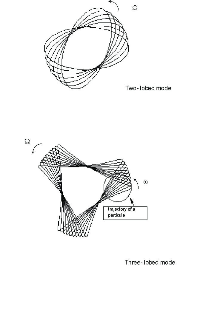
Figure 1: In the case of two-lobed mode or three-lobed mode, the drops are turning around their centre of symmetry. The trajectory of a particle is a circle represented in the case of a three-lobed mode.

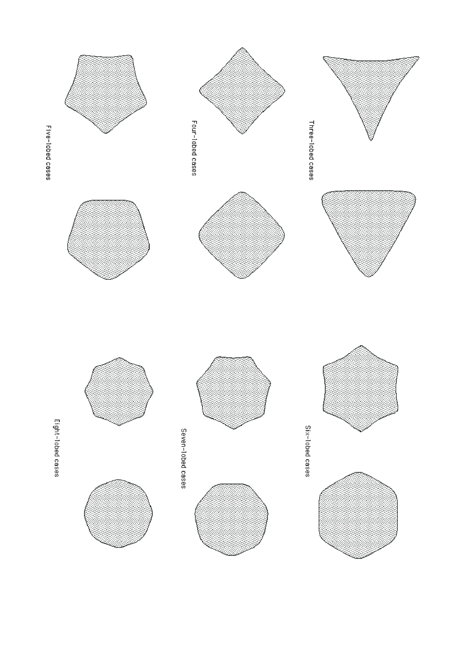
Figure 2: Two possible forms of drop are presented in cases of three-lobed to eight-lobed modes. In many cases the vibrating drops are approximately polygons which may have any of three to n sides.

References

- [1] N. J. Holter and W. R. Glasscock. Vibrations of evaporating liquid drops. The Journal of the Acoustical Society of America, 24, 6, 682-686 (1952).
- [2] J. G. Leidenfrost. De aquae communis nonnullis qualitatibus tractatus. Duisburg (1756); translated by C. Wares, Int. J. Heat Mass Transfer 15, 1153-1166 (1966).
- [3] M. Boutigny. Sur les phénomènes que présentent les corps projetés sur des surfaces chaudes. Annales de Chimie et Physique 3, IX 350-370 (1843) and 3, XI, 16-39 (1844) .
- [4] G. Flament, F. Moreaux, G. Beck. Film boiling instability at high temperature on a vertical cylinder quenched in a subcooled liquid. Int. J. Heat Mass Transfer 22, 1059-1067 (1979).
- [5] J.M. Delhaye, M. Giot, M.L. Riethmuller (eds). Thermohydraulics of two-phase systems for industrial design and nuclear engineering. Mc Graw-Hill, New York (1981).
- [6] H. Lamb, Hydrodynamics, pp. 473-475, Dover, New York (1945).
- [7] S. Iyanaga and Y. Kawada, Encyclopedic Dictionary of Mathematics. MIT Press, Cambridge, Mass. (1977).
- [8] J. Walker, The amateur scientist. Scientific American, 237, 126-131 (1977).
- [9] J. Serrin, Mathematical principle of classical fluid mechanics, Fluids dynamics1. Encyclopedia of Physics, vol. VIII/1. Springer, Berlin (1959).