Technical Report 73
IMSV, University of Bern
Adaptive Confidence Sets for the Optimal Approximating Model

Abstract

In the setting of high-dimensional linear models with Gaussian noise, we investigate the possibility of confidence statements connected to model selection. Although there exist numerous procedures for adaptive (point) estimation, the construction of adaptive confidence regions is severely limited (cf. Li, 1989). The present paper sheds new light on this gap. We develop exact and adaptive confidence sets for the best approximating model in terms of risk. One of our constructions is based on a multiscale procedure and a particular coupling argument. Utilizing exponential inequalities for noncentral $\chi^{2}$-distributions, we show that the risk and quadratic loss of all models within our confidence region are uniformly bounded by the minimal risk times a factor close to one.

t1This work was supported by the Swiss National Science Foundation.

and

1 Introduction

When dealing with a high dimensional observation vector, the natural question arises whether the data generating process can be approximated by a model of substantially lower dimension. Rather than on the true model, the focus is here on smaller ones which still contain the essential information and allow for interpretation. Typically, the models under consideration are characterized by the non-zero components of some parameter vector. Estimating the true model requires the rather idealistic situation that each component is either equals zero or has sufficiently modulus: A tiny perturbation of the parameter vector may result in the biggest model, so the question about the true model does not seem to be adequate in general. Alternatively, the model which is optimal in terms of risk appears as a target of many model selection strategies. Within a specified class of competing models, this paper is concerned with confidence regions for those approximating models which are optimal in terms of risk.

Suppose that we observe a random vector $X_{n}=(X_{in})_{i=1}^{n}$ with distribution $\mathcal{N}_{n}(\theta_{n},\sigma^{2}I_{n})$ together with an estimator $\hat{\sigma}_{n}$ for the standard deviation $\sigma>0$. Often the signal $\theta_{n}$ represents coefficients of an unknown smooth function with respect to a given orthonormal basis of functions.

There is a vast amount of literature on point estimation of $\theta_{n}$. For a given estimator $\hat{\theta}_{n}=\hat{\theta}_{n}(X_{n},\hat{\sigma}_{n})$ for $\theta_{n}$, let

$$L(\hat{\theta}_{n},\theta_{n})\ :=\ \|\hat{\theta}_{n}-\theta_{n}\|^{2}\quad\mbox{and}\quad R(\hat{\theta}_{n},\theta_{n})\ :=\ \mathbb{E}L(\hat{\theta}_{n},\theta_{n})$$

be its quadratic loss and the corresponding risk, respectively. Here $\|\cdot\|$ denotes the standard Euclidean norm of vectors. Various adaptivity results are known for this setting, often in terms of oracle inequalities. A typical result reads as follows: Let $(\check{\theta}_{n}^{(c)})_{c\in\mathcal{C}_{n}}$ be a family of candidate estimators $\check{\theta}_{n}^{(c)}=\check{\theta}_{n}^{(c)}(X_{n})$ for $\theta_{n}$, where $\sigma>0$ is temporarily assumed to be known. Then there exist estimators $\hat{\theta}_{n}$ and constants $A_{n},B_{n}=O(\log(n)^{\gamma})$ with $\gamma\geq 0$ such that for arbitrary $\theta_{n}$ in a certain set $\Theta_{n}\subset\mathbb{R}^{n}$,

$$R(\hat{\theta}_{n},\theta_{n})\ \leq\ A_{n}\inf_{c\in\mathcal{C}_{n}}R(\check{\theta}_{n}^{(c)},\theta_{n})+B_{n}\sigma^{2}.$$

Results of this type are provided, for instance, by Polyak and Tsybakov (1991) and Donoho and Johnstone (1994, 1995, 1998), in the framework of Gaussian model selection by Birg$\acute{\textrm{e}}$ and Massart (2001). The latter article copes in particular with the fact that a model is not necessarily true. Further results of this type, partly in different settings, have been provided by Stone (1984), Lepski et al. (1997), Efromovich (1998), Cai (1999, 2002), to mention just a few.

By way of contrast, when aiming at adaptive confidence sets one faces severe limitations. Here is a result of Li (1989), slightly rephrased: Suppose that $\Theta_{n}$ contains a closed Euclidean ball $B(\theta_{n}^{o},cn^{1/4})$ around some vector $\theta_{n}^{o}\in\mathbb{R}^{n}$ with radius $cn^{1/4}>0$. Still assuming $\sigma$ to be known, let $\hat{D}_{n}=\hat{D}_{n}(X_{n})\subset\Theta_{n}$ be a $(1-\alpha)$-confidence set for $\theta_{n}\in\Theta_{n}$. Such a confidence set may be used as a test of the (Bayesian) null hypothesis that $\theta_{n}$ is uniformly distributed on the sphere $\partial B(\theta_{n}^{o},cn^{1/4})$ versus the alternative that $\theta_{n}=\theta_{n}^{o}$: We reject this null hypothesis at level $\alpha$ if $\|\eta-\theta_{n}^{o}\|<cn^{1/4}$ for all $\eta\in\hat{D}_{n}$. Since this test cannot have larger power than the corresponding Neyman-Pearson test,

$$\mathbb{P}_{\theta_{n}^{o}}\biggl{(}\sup_{\eta\in\hat{D}_{n}}\|\eta-\theta_{n}^{o}\|_{n}<cn^{1/4}\biggr{)} \leq \mathbb{P}\Bigl{(}S_{n}^{2}\leq\chi_{n;\alpha}^{2}(c^{2}n^{1/2}/\sigma^{2})\Bigr{)}\quad(S_{n}^{2}\sim\chi_{n}^{2})$$

$$= \Phi\Bigl{(}\Phi^{-1}(\alpha)+2^{-1/2}c^{2}/\sigma^{2}\Bigr{)}+o(1),$$

where $\chi_{n;\alpha}^{2}(\delta^{2})$ stands for the $\alpha$-quantile of the noncentral chi-squared distribution with $n$ degrees of freedom and noncentrality parameter $\delta^{2}$. Throughout this paper, asymptotic statements refer to $n\to\infty$. The previous inequality entails that no reasonable confidence set has a diameter of order $o_{p}(n^{1/4})$ uniformly over the parameter space $\Theta_{n}$, as long as the latter is sufficiently large. Despite these limitations, there is some literature on confidence sets in the present or similar settings; see for instance Beran (1996, 2000), Beran and Dümbgen (1998) and Genovese and Wassermann (2005).

Improving the rate of $O_{p}(n^{1/4})$ is only possible via additional constraints on $\theta_{n}$, i.e. considering substantially smaller sets $\Theta_{n}$. For instance, Baraud (2004) developed nonasymptotic confidence regions which perform well on finitely many linear subspaces. Robins and van der Vaart (2006) construct confidence balls via sample splitting which adapt to some extent to the unknown “smoothness” of $\theta_{n}$. In their context, $\Theta_{n}$ corresponds to a Sobolev smoothness class with given parameter $(\beta,L)$. However, adaptation in this context is possible only within a range $[\beta,2\beta]$. Independently, Cai and Low (2006) treat the same problem in the special case of the Gaussian white noise model, obtaining the same kind of adaptivity in the broader scale of Besov bodies. Other possible constraints on $\theta_{n}$ are so-called shape constraints; see for instance Cai and Low (2007), Dümbgen (2003) or Hengartner and Stark (1995).

The question is whether one can bridge this gap between confidence sets and point estimators. More precisely, we would like to understand the possibility of adaptation for point estimators in terms of some confidence region for the set of all optimal candidate estimators $\check{\theta}_{n}^{(c)}$. That means, we want to construct a confidence region $\hat{\mathcal{K}}_{n,\alpha}=\hat{\mathcal{K}}_{n,\alpha}(X_{n},\hat{\sigma}_{n})\subset\mathcal{C}_{n}$ for the set

$$\mathcal{K}_{n}(\theta_{n})\,:= \,\mathop{\rm argmin}_{c\in\mathcal{C}_{n}}R(\check{\theta}_{n}^{(c)})$$

$$= \,\Big{\{}c\in\mathcal{C}_{n}:\,R(\check{\theta}_{n}^{(c)},\theta_{n})\leq R(\check{\theta}_{n}^{(c^{\prime})},\theta_{n})\,\text{for all}\,c^{\prime}\in\mathcal{C}_{n}\Big{\}}$$

such that for arbitrary $\theta_{n}\in\mathbb{R}^{n}$,

$$\mathbb{P}_{\theta_{n}}\Bigl{(}\mathcal{K}_{n}(\theta_{n})\subset\hat{\mathcal{K}}_{n,\alpha}\Bigr{)}\ \geq\ 1-\alpha$$ (1)

and

$$\left.\begin{array}[]{c}\displaystyle\max_{c\in\hat{\mathcal{K}}_{n,\alpha}}\,R(\check{\theta}_{n}^{(c)},\theta_{n})\\ \displaystyle\max_{c\in\hat{\mathcal{K}}_{n,\alpha}}\,L(\check{\theta}_{n}^{(c)},\theta_{n})\end{array}\right\}\ =\ O_{p}(A_{n})\min_{c\in\mathcal{C}_{n}}\,R(\check{\theta}_{n}^{(c)},\theta_{n})+O_{p}(B_{n})\sigma^{2}.$$ (2)

Solving this problem means that statistical inference about differences in the performance of estimators is possible, although inference about their risk and loss is severely limited. In some settings, selecting estimators out of a class of competing estimators entails estimating implicitly an unknown regularity or smoothness class for the underlying signal $\theta_{n}$. Computing a confidence region for good estimators is particularly suitable in situations in which several good candidate estimators fit the data equally well although they look different. This aspect of exploring various candidate estimators is not covered by the usual theory of point estimation.

Note that our confidence region $\hat{\mathcal{K}}_{n,\alpha}$ is required to contain the whole set $\mathcal{K}_{n}(\theta_{n})$, not just one element of it, with probability at least $1-\alpha$. The same requirement is used by Futschik (1999) for inference about the argmax of a regression function.

The remainder of this paper is organized as follows. For the reader’s convenience our approach is first described in a simple toy model in Section 2. In Section 3 we develop and analyze an explicit confidence region $\hat{\mathcal{K}}_{n,\alpha}$ related to $\mathcal{C}_{n}:=\{0,1,\ldots,n\}$ with candidate estimators

$$\check{\theta}_{n}^{(k)}\ :=\ \bigl{(}1\{i\leq k\}X_{in}\bigr{)}_{i=1}^{n}.$$

These correspond to a standard nested sequence of approximating models. Section 4 discusses richer families of candidate estimators.

All proofs and auxiliary results are deferred to Sections 5 and 6.

2 A toy problem

Suppose we observe a stochastic process $Y=(Y(t))_{t\in[0,1]}$, where

$$Y(t)\ =\ F(t)+W(t),\quad t\in[0,1],$$

with an unknown fixed continuous function $F$ on $[0,1]$ and a Brownian motion $W=(W(t))_{t\in[0,1]}$. We are interested in the set

$$\SS(F)\ :=\ \mathop{\rm argmin}_{t\in[0,1]}F(t).$$

Precisely, we want to construct a $(1-\alpha)$-confidence region $\hat{\SS}_{\alpha}=\hat{\SS}_{\alpha}(Y)\subset[0,1]$ for $\SS(F)$ in the sense that

$$P\bigl{(}\SS(F)\subset\hat{\SS}_{\alpha}\bigr{)}\ \geq\ 1-\alpha,$$ (3)

regardless of $F$. To construct such a confidence set we regard $Y(s)-Y(t)$ for arbitrary different $s,t\in[0,1]$ as a test statistic for the null hypothesis that $s\in\SS(F)$, i.e. large values of $Y(s)-Y(t)$ give evidence for $s\not\in\SS(F)$.

A first naive proposal is the set

$$\hat{\SS}_{\alpha}^{\rm naive}\ :=\ \Bigl{\{}s\in[0,1]:Y(s)\leq\min_{[0,1]}Y+\kappa_{\alpha}^{\rm naive}\Bigr{\}}$$

with $\kappa_{\alpha}^{\rm naive}$ denoting the $(1-\alpha)$-quantile of $\max_{[0,1]}W-\min_{[0,1]}W$.

Here is a refined version based on results of Dümbgen and Spokoiny (2001): Let $\kappa_{\alpha}$ be the $(1-\alpha)$-quantile of

$$\sup_{s,t\in[0,1]}\biggl{(}\frac{|W(s)-W(t)|}{\sqrt{|s-t|}}-\sqrt{2\log(e/\arrowvert s-t\arrowvert)}\biggr{)}.$$ (4)

Then constraint (3) is satisfied by the confidence region $\hat{\SS}_{\alpha}$ which consists of all $s\in[0,1]$ such that

$$Y(s)\leq Y(t)+\sqrt{|s-t|}\Bigl{(}\sqrt{2\log(e/\arrowvert s-t\arrowvert)}\,+\,\kappa_{\alpha}\Bigr{)}\ \text{for all}\ t\in[0,1].$$

To illustrate the power of this method, consider for instance a sequence of functions $F=F_{n}=c_{n}F_{o}$ with positive constants $c_{n}\to\infty$ and a fixed continuous function $F_{o}$ with unique minimizer $s_{o}$. Suppose that

$$\lim_{t\to s_{o}}\frac{F_{o}(t)-F_{o}(s_{o})}{|t-s_{o}|^{\gamma}}\ =\ 1$$

for some $\gamma>1/2$. Then the naive confidence region satisfies only

$$\max_{t\in\hat{\SS}_{\alpha}^{\rm naive}}\,|t-s_{o}|\ =\ O_{p}\bigl{(}c_{n}^{-1/\gamma}\bigr{)},$$ (5)

whereas

$$\max_{t\in\hat{\SS}_{\alpha}}\,|t-s_{o}|\ =\ O_{p}\Bigl{(}\log(c_{n})^{1/(2\gamma-1)}c_{n}^{-2/(2\gamma-1)}\Bigr{)}.$$ (6)

3 Confidence regions for nested approximating models

As in the introduction let $X_{n}=\theta_{n}+\epsilon_{n}$ denote the $n$-dimensional observation vector with $\theta_{n}\in\mathbb{R}^{n}$ and $\epsilon_{n}\sim\mathcal{N}_{n}(0,\sigma^{2}I_{n})$. For any candidate estimator $\check{\theta}_{n}^{(k)}=\bigl{(}1\{i\leq k\}X_{in}\bigr{)}_{i=1}^{n}$ the loss is given by

$$L_{n}(k):=L(\check{\theta}_{n}^{(k)},\theta_{n})\ =\ \sum_{i=k+1}^{n}\theta_{in}^{2}+\sum_{i=1}^{k}(X_{in}-\theta_{in})^{2}$$

with corresponding risk

$$R_{n}(k):=R(\check{\theta}_{n}^{(k)},\theta_{n})\ =\ \sum_{i=k+1}^{n}\theta_{in}^{2}+k\sigma^{2}.$$

Model selection usually aims at estimating a candidate estimator which is optimal in terms of risk. Since the risk depends on the unknown signal and therefore is not available, the selection procedure minimizes an unbiased risk estimator instead. In the sequel, the bias-corrected risk estimator for the candidate $\check{\theta}_{n}^{(k)}$ is defined as

$$\hat{R}_{n}(k)\ :=\ \sum_{i=k+1}^{n}(X_{in}^{2}-\hat{\sigma}_{n}^{2})+k\hat{\sigma}_{n}^{2},$$

where $\hat{\sigma}_{n}^{2}$ is a variance estimator satisfying the subsequent condition.

(A) $\hat{\sigma}_{n}^{2}$ and $X_{n}$ are stochastically independent with

$$\frac{m\hat{\sigma}_{n}^{2}}{\sigma^{2}}\ \sim\ \chi_{m}^{2},$$

where $1\leq m=m_{n}\leq\infty$ with $m=\infty$ meaning that $\sigma$ is known, i.e. $\hat{\sigma}_{n}^{2}\equiv\sigma^{2}$. For asymptotic statements, it is generally assumed that

$$\beta_{n}^{2}\ :=\ \frac{2n}{m_{n}}\ =\ O(1)$$

unless stated otherwise.

Example.

Suppose that we observe $Y=M\eta+\delta$ with given design matrix $M\in\mathbb{R}^{(n+m)\times n}$ of rank $n$, unknown parameter vector $\eta\in\mathbb{R}^{n}$ and unobserved error vector $\delta\sim\mathcal{N}_{n+m}(0,\sigma^{2}I_{n+m})$. Then the previous assumptions are satisfied by $X_{n}:=(M^{\top}M)^{1/2}\hat{\eta}$ with $\hat{\eta}:=(M^{\top}M)^{-1}M^{\top}Y$ and $\hat{\sigma}_{n}^{2}:=\|Y-M\hat{\eta}\|^{2}/m$, where $\theta_{n}:=(M^{\top}M)^{1/2}\eta$.

Important for our analysis is the behavior of the centered and rescaled difference process $\hat{D}_{n}=\bigl{(}\hat{D}_{n}(j,k)\bigr{)}_{0\leq j<k\leq n}$ with

$$\hat{D}_{n}(j,k) := \frac{\hat{R}_{n}(j)-\hat{R}_{n}(k)-R_{n}(j)+R_{n}(k)}{\hat{\sigma}_{n}^{2}\big{(}4\Arrowvert\theta_{n}/\sigma\Arrowvert^{2}+2n\big{)}^{1/2}}$$

$$= \frac{\sum_{i=j+1}^{k}(X_{in}^{2}-\sigma^{2}-\theta_{in}^{2})-2(k-j)(\hat{\sigma}^{2}-\sigma^{2})}{\hat{\sigma}_{n}^{2}\big{(}4\Arrowvert\theta_{n}/\sigma\Arrowvert^{2}+2n\big{)}^{1/2}}.$$

One may also write $\hat{D}_{n}(j,k)=(\hat{\sigma}_{n}/\sigma)^{-2}\bigl{(}D_{n}(j,k)+V_{n}(j,k)\bigr{)}$ with

$$D_{n}(j,k)\, :=\,\frac{1}{\sqrt{4\Arrowvert\theta_{n}/\sigma\Arrowvert^{2}+2n}}\sum_{i=j+1}^{k}\Bigl{(}2(\theta_{in}/\sigma)(\epsilon_{in}/\sigma)+(\epsilon_{in}/\sigma)^{2}-1\Bigr{)},$$ (7)

$$V_{n}(j,k)\, :=\,\big{(}4\Arrowvert\theta_{n}/\sigma\Arrowvert^{2}+2n\big{)}^{-1/2}2(k-j)(1-\hat{\sigma}^{2}/\sigma^{2})$$ (8)

This representation shows that the distribution of $\hat{D}_{n}$ depends on the degrees of freedom, $m$, and the unknown “signal-to-noise vector” $\theta_{n}/\sigma$. The process $D_{n}$ consists of partial sums of the independent, but in general non-identically distributed random variables $2(\theta_{in}/\sigma)(\epsilon_{in}/\sigma)+(\epsilon_{in}/\sigma)^{2}-1$. The standard deviation of $D_{n}(j,k)$ is given by

$$\tau_{n}(j,k)\ :=\ \frac{1}{\sqrt{4\Arrowvert\theta_{n}/\sigma\Arrowvert^{2}+2n}}\Bigl{(}\sum_{i=j+1}^{k}\bigl{(}4\theta_{in}^{2}/\sigma^{2}+2\bigr{)}\Bigr{)}^{1/2}.$$

Note that $\tau_{n}(0,n)=1$ by construction. To imitate the more powerful confidence region of Section 2 based on the multiscale approach, one needs a refined analysis of the increment process $\hat{D}_{n}$. Since this process does not have subgaussian tails, the standardization is more involved than the correction in (4).

Theorem 1.

Define $\Gamma_{n}(j,k):=\big{(}2\log\big{(}e/\tau_{n}(j,k)^{2}\big{)}^{1/2}$ for $0\leq j<k\leq n$. Then

$$\sup_{0\leq j<k\leq n}\frac{|\hat{D}_{n}(j,k)|}{\tau_{n}(j,k)}\ \leq\ \sqrt{32}\,\log n+O_{p}(1),$$

and for any fixed $c>2$,

$$\hat{d}_{n}:=\sup_{0\leq j<k\leq n}\Biggl{(}\frac{|\hat{D}_{n}(j,k)|}{\tau_{n}(j,k)}\,-\,\Gamma_{n}(j,k)\,-\,\frac{c\cdot\Gamma_{n}(j,k)^{2}}{\big{(}4\Arrowvert\theta_{n}/\sigma\Arrowvert^{2}+2n\big{)}^{1/2}\tau_{n}(j,k)}\Biggr{)}^{+}$$

is bounded in probability. In case of $\|\theta_{n}\|^{2}=O(n)$, $\mathcal{L}(\hat{d}_{n})$ is weakly approximated by the law of

$$\delta_{n}:=\sup_{0\leq j<k\leq n}\biggl{(}\frac{|\Delta_{n}(j,k)|}{\tau_{n}(j,k)}-\Gamma_{n}(j,k)\biggr{)}^{+},$$

where

$$\Delta_{n}(j,k)\ =\ W(\tau_{n}(0,k)^{2})-W(\tau_{n}(0,j)^{2})-\frac{2\beta_{n}(k-j)}{\sqrt{n}\,\big{(}4\Arrowvert\theta_{n}/\sigma\Arrowvert^{2}+2n\big{)}^{1/2}}\,Z$$

with a standard Brownian motion $W$ and a random variable $Z\sim\mathcal{N}(0,1)$ independent of $W$.

The limiting distribution indicates that the additive correction term in the definition of $\hat{d}_{n}$ cannot be chosen essentially smaller. It will play a crucial role for the efficiency of the confidence region.

To construct a confidence set for $\mathcal{K}_{n}(\theta_{n})$ by means of $\hat{d}_{n}$, we are facing the problem that the auxiliary function $\tau_{n}(\cdot,\cdot)$ depends on the unknown signal-to-noise vector $\theta_{n}/\sigma$. In fact, knowing $\tau_{n}$ would imply knowledge of $\mathcal{K}_{n}(\theta_{n})$ already. A natural approach is to replace the quantities which are dependent on the unknown parameter by suitable estimates. A common estimator of the variance $\tau_{n}(j,k)^{2}$, $j<k$, is given by

$$\hat{\tau}_{n}(j,k)^{2}\ :=\ \bigg{\{}\sum_{i=1}^{n}\Bigl{(}4(X_{in}^{2}/\hat{\sigma}_{n}^{2}-1)+2\Bigr{)}\biggr{\}}^{-1}\sum_{i=j+1}^{k}\Bigl{(}4(X_{in}^{2}/\hat{\sigma}_{n}^{2}-1)+2\Bigr{)}.$$

However, using such an estimator does not seem to work since

$$\sup_{0\leq j<k\leq n}\,\Bigl{|}\frac{\hat{\tau}_{n}(j,k)}{\tau_{n}(j,k)}-1\Bigr{|}\ \not\longrightarrow_{p}\ 0$$

as $n$ goes to infinity. This can be verified by noting that the (rescaled) numerator of $\bigl{(}\hat{\tau}_{n}(j,k)^{2}\bigr{)}_{0\leq j<k\leq n}$ is, up to centering, essentially of the same structure as the rescaled difference process $\hat{D}_{n}$ itself.

The least favourable case of constant risk

The problem of estimating the set $\arg\min_{k}R_{n}(k)$ can be cast into our toy model where $Y(t)$, $F(t)$ and $W(t)$ correspond to $\hat{R}_{n}(k)$, $R_{n}(k)$ and the difference $\hat{R}_{n}(k)-R_{n}(k)$, respectively. One may expect that the more distinctive the global minima are, the easier it is to identify their location. Hence the case of constant risks appears to be least favourable, corresponding to a signal

$$\theta_{n}^{*}\ :=\ \bigl{(}\pm\sigma\bigr{)}_{i=1}^{n},$$

In this situation, each candidate estimator $\check{\theta}_{n}^{(k)}$ has the same risk of $n\sigma^{2}$.

A related consideration leading to an explicit procedure is as follows: For fixed indices $0\leq j<k\leq n$,

$$R_{n}(j)-R_{n}(k)\ =\ \sum_{i=j+1}^{k}\theta_{in}^{2}-(k-j)\sigma^{2},$$

and if Assumption (A) is satisfied, the statistic

$$T_{jkn}\ :=\ \frac{\sum_{i=j+1}^{k}X_{in}^{2}}{(k-j)\hat{\sigma}_{n}^{2}}\ =\ 2-\frac{\hat{R}_{n}(k)-\hat{R}_{n}(j)}{(k-j)\hat{\sigma}_{n}^{2}}$$

has a noncentral (in the numerator) $F$-distribution

$$F_{k-j,m}\biggl{(}\frac{\sum_{i=j+1}^{k}\theta_{in}^{2}}{\sigma^{2}}\biggr{)}=F_{k-j,m}\biggl{(}k-j+\frac{R_{n}(j)-R_{n}(k)}{\sigma^{2}}\biggr{)}$$

with $k-j$ and $m$ degrees of freedom. Thus large or small values of $T_{jkn}$ give evidence for $R_{n}(j)$ being larger or smaller, respectively, than $R_{n}(k)$. Precisely,

$$\mathcal{L}_{\theta_{n}}(T_{jkn})\ \begin{cases}\leq_{\rm st.}\ \mathcal{L}_{\theta_{n}^{*}}(T_{jkn})&\mbox{whenever }j\in\mathcal{K}_{n}(\theta_{n}),\\ \geq_{\rm st.}\ \mathcal{L}_{\theta_{n}^{*}}(T_{jkn})&\mbox{whenever }k\in\mathcal{K}_{n}(\theta_{n}).\end{cases}$$

Note that this stochastic ordering remains valid if $\hat{\sigma}_{n}^{2}$ is just independent from $X_{n}$, i.e. also under the more general requirement of the remark at the end of this section. Via suitable coupling of Poisson mixtures of central $\chi^{2}$-distributed random variables, this observation is extended to a coupling for the whole process $\big{(}T_{jkn}\big{)}_{0\leq j<k\leq n}$:

Proposition 2 (Coupling).

For any $\theta_{n}\in\mathbb{R}^{n}$ there exists a probability space with random variables $\bigl{(}\tilde{T}_{jkn}\bigr{)}_{0\leq j<k\leq n}$ and $\bigl{(}\tilde{T}^{*}_{jkn}\bigr{)}_{0\leq j<k\leq n}$ such that

$$\mathcal{L}\Bigl{(}\bigl{(}\tilde{T}_{jkn}\bigr{)}_{0\leq j<k\leq n}\Bigr{)} = \mathcal{L}_{\theta_{n}}\Bigl{(}\bigl{(}T_{jkn}\bigr{)}_{0\leq j<k\leq n}\Bigr{)},$$

$$\mathcal{L}\Bigl{(}\bigl{(}\tilde{T}^{*}_{jkn}\bigr{)}_{0\leq j<k\leq n}\Bigr{)} = \mathcal{L}_{\theta_{n}^{*}}\Bigl{(}\bigl{(}T_{jkn}\bigr{)}_{0\leq j<k\leq n}\Bigr{)},$$

and for arbitrary indices $0\leq j<k\leq n$,

$$\tilde{T}_{jkn}\ \begin{cases}\leq\ \tilde{T}_{jkn}^{*}&\mbox{whenever }j\in\mathcal{K}_{n}(\theta_{n}),\\ \geq\ \tilde{T}_{jkn}^{*}&\mbox{whenever }k\in\mathcal{K}_{n}(\theta_{n}).\end{cases}$$

As a consequence of Proposition 2, we can define a confidence set for $\mathcal{K}_{n}(\theta_{n})$, based on this least favourable case. Let $\kappa_{n,\alpha}$ denote the $(1-\alpha)$-quantile of $\mathcal{L}_{\theta_{n}^{*}}(\hat{d}_{n})$, where for simplicity $c:=3$ in the definition of $\hat{d}_{n}$. Note also that $\tau_{n}(j,k)^{2}=(k-j)/n$ in case of $\theta_{n}=\theta_{n}^{*}$. Motivated by the procedure in Section 2 and Theorem 1, we define

$$\hat{\mathcal{K}}_{n,\alpha} := \Bigl{\{}j:\,\hat{R}_{n}(j)\leq\hat{R}_{n}(k)+\hat{\sigma}_{n}^{2}|k-j|c_{jkn}\ \text{for all}\ k\neq j\Bigr{\}}$$

$$\,= \bigl{\{}j:\,T_{ijn}\geq 2-c_{ijn}\ \text{for all}\ i<j,$$

$$\qquad\qquad\qquad\qquad\quad T_{jkn}\leq 2+c_{jkn}\ \text{for all}\ k>j\bigr{\}}$$

with

$$c_{jkn}=c_{jkn,\alpha}\ :=\ \sqrt{\frac{6}{|k-j|}}\biggl{(}\Gamma\Bigl{(}\frac{k-j}{n}\Bigr{)}+\kappa_{n,\alpha}\bigg{)}+\frac{3}{|k-j|}\Gamma\Bigl{(}\frac{k-j}{n}\Bigr{)}^{2}.$$

Theorem 3.

Let $(\theta_{n})_{n\in\mathbb{N}}$ be arbitrary. With $\hat{\mathcal{K}}_{n,\alpha}$ as defined above,

$$\mathbb{P}_{\theta_{n}}\Bigl{(}\mathcal{K}_{n}(\theta_{n})\not\subset\hat{\mathcal{K}}_{n,\alpha}\Bigr{)}\ \leq\ \alpha.$$

In case of $\beta_{n}\to 0$ (i.e. $n/m\to 0$), the critical values $\kappa_{n,\alpha}$ converge to the critical value $\kappa_{\alpha}$ introduced in Section 2. In general, $\kappa_{n,\alpha}=O(1)$, and the confidence regions $\hat{\mathcal{K}}_{n,\alpha}$ satisfy the oracle inequalities

$$\max_{k\in\hat{\mathcal{K}}_{n,\alpha}}R_{n}(k)\ \leq\ \min_{j\in\mathcal{C}_{n}}\,R_{n}(j)\ +\ \bigl{(}4\sqrt{3}+o_{p}(1)\bigr{)}\sqrt{\sigma^{2}\log(n)\min_{j\in\mathcal{C}_{n}}R_{n}(j)}$$ (10)

$$+\ O_{p}\bigl{(}\sigma^{2}\log n\bigr{)}$$

and

$$\max_{k\in\hat{\mathcal{K}}_{n,\alpha}}L_{n}(k)\ \leq\ \min_{j\in\mathcal{C}_{n}}\,L_{n}(j)\ +\ O_{p}\Bigl{(}\sqrt{\sigma^{2}\log(n)\min_{j\in\mathcal{C}_{n}}L_{n}(j)}\Bigr{)}$$ (11)

$$+\ O_{p}\bigl{(}\sigma^{2}\log n\bigr{)}.$$

Remark (Dependence on $\alpha$)

The proof reveals a refined version of the bounds in Theorem 3 in case of signals $\theta_{n}$ such that

$$\log(n)^{3}\ =\ O\Bigl{(}\min_{j\in\mathcal{C}_{n}}\,R_{n}(j)\Bigr{)}.$$

Let $0<\alpha(n)\to 0$ such that $\kappa_{n,\alpha(n)}^{6}=O\Bigl{(}\min_{j\in\mathcal{C}_{n}}\,R_{n}(j)\Bigr{)}$. Then

$$\max_{k\in\hat{\mathcal{K}}_{n,\alpha}}\,R_{n}(k) \leq \min_{j\in\mathcal{C}_{n}}\,R_{n}(j)$$

$$+\ \Bigl{(}4\sqrt{3}\sqrt{\log n}+2\sqrt{6}\,\kappa_{n,\alpha}+O_{p}(1)\Bigr{)}\sqrt{\sigma^{2}\min_{j\in\mathcal{C}_{n}}R_{n}(j)}$$

uniformly in $\alpha\geq\alpha(n)$.

Remark (Variance estimation)

Instead of Condition (A), one may require more generally that $\hat{\sigma}_{n}^{2}$ and $X_{n}$ are independent with

$$\sqrt{n}\Bigl{(}\frac{\hat{\sigma}_{n}^{2}}{\sigma^{2}}-1\Bigr{)}\ \to_{D}\ \mathcal{N}(0,\beta^{2})$$

for a given $\beta\geq 0$. This covers, for instance, estimators used in connection with wavelets. There $\sigma$ is estimated by the median of some high frequency wavelet coefficients divided by the normal quantile $\Phi^{-1}(3/4)$. Theorem 1 continues to hold, and the coupling extends to this situation, too, with $S^{2}$ in the proof being distributed as $n\hat{\sigma}_{n}^{2}$. Under this assumption on the external variance estimator, the confidence region $\hat{\mathcal{K}}_{n,\alpha}$, defined with $m:=\lfloor 2n/\beta^{2}\rfloor$, is at least asymptotically valid and satisfies the above oracle inequalities as well.

4 Confidence sets in case of larger families of candidates

The previous result relies strongly on the assumption of nested models. It is possible to obtain confidence sets for the optimal approximating models in a more general setting, albeit the resulting oracle property is not as strong as in the nested case. In particular, we can no longer rely on a coupling result but need a different construction. For the reader’s convenience, we focus on the case of known $\sigma$, i.e. $m=\infty$; see also the remark at the end of this section.

Let $\mathcal{C}_{n}$ be a family of index sets $C\subset\{1,2,\ldots,n\}$ with candidate estimators

$$\check{\theta}^{(C)}\ :=\ \bigl{(}1\{i\in C\}X_{in}\bigr{)}_{i=1}^{n}$$

and corresponding risks

$$R_{n}(C):=R(\check{\theta}^{(C)},\theta_{n})\ =\ \sum_{i\not\in C}\theta_{in}^{2}+|C|\sigma^{2},$$

where $|S|$ denotes the cardinality of a set $S$. For two index sets $C$ and $D$,

$$\sigma^{-2}\bigl{(}R_{n}(D)-R_{n}(C)\bigr{)}\ =\ \delta_{n}^{2}(C\setminus D)-\delta_{n}^{2}(D\setminus C)+|D|-|C|$$

with the auxiliary quantities

$$\delta_{n}^{2}(J)\ :=\ \sum_{i\in J}\theta_{in}^{2}/\sigma^{2},\quad J\subset\{1,2,\ldots,n\}.$$

Hence we aim at simultaneous $(1-\alpha)$-confidence intervals for these noncentrality parameters $\delta_{n}(J)$, where $J\in\mathcal{M}_{n}:=\{D\setminus C:C,D\in\mathcal{C}_{n}\}$. To this end we utilize the fact that

$$T_{n}(J)\ :=\ \frac{1}{\sigma^{2}}\sum_{i\in J}X_{in}^{2}$$

has a $\chi_{|J|}^{2}(\delta_{n}^{2}(J))$-distribution. We denote the distribution function of $\chi_{k}^{2}(\delta^{2})$ by $F_{k}(\cdot\mid\delta^{2})$. Now let $M_{n}:=|\mathcal{M}_{n}|-1\leq|\mathcal{C}_{n}|(|\mathcal{C}_{n}|-1)$, the number of nonvoid index sets $J\in\mathcal{M}_{n}$. Then with probability at least $1-\alpha$,

$$\alpha/(2M_{n})\leq F_{|J|}\bigl{(}T_{n}(J)\,\big{|}\,\delta_{n}^{2}(J)\bigr{)}\leq 1-\alpha/(2M_{n})\quad\text{for}\ \emptyset\neq J\in\mathcal{M}_{n}.$$ (12)

Since $F_{|J|}(T_{n}(J)\mid\delta^{2})$ is strictly decreasing in $\delta^{2}$ with limit $0$ as $\delta^{2}\to\infty$, (12) entails the simultaneous $(1-\alpha)$-confidence intervals $\bigl{[}\hat{\delta}_{n,\alpha,l}^{2}(J),\hat{\delta}_{n,\alpha,u}^{2}(J)\bigr{]}$ for all parameters $\delta_{n}^{2}(J)$ as follows: We set $\hat{\delta}_{n,\alpha,l}^{2}(\emptyset):=\hat{\delta}_{n,\alpha,u}^{2}(\emptyset):=0$, while for nonvoid $J$,

$$\hat{\delta}_{n,\alpha,l}^{2}(J) := \min\Bigl{\{}\delta^{2}\geq 0:F_{|J|}\bigl{(}T_{n}(J)\,\big{|}\,\delta^{2}\bigr{)}\leq 1-\alpha/(2M_{n})\Bigr{\}},$$ (13)

$$\hat{\delta}_{n,\alpha,u}^{2}(J) := \max\Bigl{\{}\delta^{2}\geq 0:F_{|J|}\bigl{(}T_{n}(J)\,\big{|}\,\delta^{2}\bigr{)}\geq\alpha/(2M_{n})\Bigr{\}}.$$ (14)

By means of these bounds, we may claim with confidence $1-\alpha$ that for arbitrary $C,D\in\mathcal{C}_{n}$ the normalized difference $(n/\sigma^{2})\bigl{(}R_{n}(D)-R_{n}(C)\bigr{)}$ is at most $\hat{\delta}_{n,\alpha,u}^{2}(C\setminus D)-\hat{\delta}_{n,\alpha,l}^{2}(D\setminus C)+|D|-|C|$. Thus a $(1-\alpha)$-confidence set for $\mathcal{K}_{n}(\theta_{n})=\mathop{\rm argmin}_{C\in\mathcal{C}_{n}}\,R_{n}(C)$ is given by

$$\hat{\mathcal{K}}_{n,\alpha}\ :=\ \Bigl{\{}C\in\mathcal{C}_{n}:\hat{\delta}_{n,\alpha,u}^{2}(C\setminus D)-\hat{\delta}_{n,\alpha,l}^{2}(D\setminus C)+|D|-|C|\geq 0\ \text{for all}\ D\in\mathcal{C}_{n}\Bigr{\}}.$$

These confidence sets $\hat{\mathcal{K}}_{n,\alpha}$ satisfy the following oracle inequalities:

Theorem 4.

Let $(\theta_{n})_{n\in\mathbb{N}}$ be arbitrary, and suppose that $\log|\mathcal{C}_{n}|=o(n)$. Then

$$\max_{C\in\hat{\mathcal{K}}_{n,\alpha}}\,R_{n}(C)\ \leq\ \min_{D\in\mathcal{C}_{n}}\,R_{n}(D)\ +\ O_{p}\biggl{(}\sqrt{\sigma^{2}\log(\arrowvert\mathcal{C}_{n}\arrowvert)\min_{D\in\mathcal{C}_{n}}\,R_{n}(D)}\biggr{)}$$

$$+\ O_{p}\big{(}\sigma^{2}\log\arrowvert\mathcal{C}_{n}\arrowvert\big{)}$$

and

$$\max_{C\in\hat{\mathcal{K}}_{n,\alpha}}\,L_{n}(C)\ \leq\ \min_{D\in\mathcal{C}_{n}}\,L_{n}(D)\ +\ O_{p}\biggl{(}\sqrt{\sigma^{2}\log(\arrowvert\mathcal{C}_{n}\arrowvert)\min_{D\in\mathcal{C}_{n}}\,L_{n}(D)}\biggr{)}$$

$$+\ O_{p}\big{(}\sigma^{2}\log\arrowvert\mathcal{C}_{n}\arrowvert\big{)}.$$

Remark.

The upper bounds in Theorem 4 are of the form

$$\rho_{n}\Bigl{(}1+O_{p}\Bigl{(}\sqrt{\sigma^{2}\log(\arrowvert\mathcal{C}_{n}\arrowvert)/\rho_{n}}+\sigma^{2}\log(\arrowvert\mathcal{C}_{n}\arrowvert)/\rho_{n}\Bigr{)}\Bigr{)}$$

with $\rho_{n}$ denoting minimal risk or minimal loss. Thus Theorem 4 entails that the maximal risk (loss) over $\hat{\mathcal{K}}_{n,\alpha}$ exceeds the minimal risk (loss) only by a factor close to one, provided that the minimal risk (loss) is substantially larger than $\sigma^{2}\log\arrowvert\mathcal{C}_{n}\arrowvert$.

Remark (Suboptimality in case of nested models)

In case of nested models, the general construction is suboptimal in the factor of the leading (in most cases) term $\sqrt{\min_{j}R_{n}(j)}$. Following the proof carefully and using that $\sigma^{2}\log\arrowvert\mathcal{C}_{n}\arrowvert=2\sigma^{2}\log n\,+\,O(1)$ in this special setting, one may verify that

$$\max_{k\in\hat{\mathcal{K}}_{n,\alpha}}\,R_{n}(k)\ \leq\ \min_{j\in\mathcal{C}_{n}}\,R_{n}(j)\ +\ \bigl{(}4\sqrt{8}+o_{p}(1)\bigr{)}\sqrt{\sigma^{2}\log(n)\min_{j\in\mathcal{C}_{n}}\,R_{n}(j)}$$

$$+\ O_{p}\big{(}\sigma^{2}\log n\big{)}.$$

The intrinsic reason is that the general procedure does not assume any structure of the family of candidate estimators. Hence advanced multiscale theory is not applicable.

Remark.

In case of unknown $\sigma$, let $\alpha^{\prime}:=1-(1-\alpha)^{1/2}$. Then with probability at least $1-\alpha^{\prime}$,

$$\alpha^{\prime}/2\ \leq\ F_{m}\bigl{(}m(\hat{\sigma}_{n}/\sigma)^{2}\,\big{|}\,0\bigr{)}\ \leq\ 1-\alpha^{\prime}/2.$$

The latter inequalities entail that $(\sigma/\hat{\sigma}_{n})^{2}$ lies between $\tau_{n,\alpha,l}:=m/\chi_{m;1-\alpha^{\prime}/2}$ and $\tau_{n,\alpha,u}:=m/\chi_{m;\alpha^{\prime}/2}^{2}$. Then we obtain simultaneous $(1-\alpha)$-confidence bounds $\hat{\delta}_{n,\alpha,l}^{2}(J)$ and $\hat{\delta}_{n,\alpha,u}^{2}(J)$ as in (13) and (14) by replacing $\alpha$ with $\alpha^{\prime}$ and $T_{n}(J)$ with

$$\frac{\tau_{n,\alpha,l}}{\hat{\sigma}_{n}^{2}}\sum_{i\in J}X_{in}^{2}\quad\text{and}\quad\frac{\tau_{n,\alpha,u}}{\hat{\sigma}_{n}^{2}}\sum_{i\in J}X_{in}^{2},$$

respectively. The conclusions of Theorem 4 continue to hold, as long as $n/m_{n}=O(1)$.

5 Proofs

5.1 Proof of (5) and (6)

Note first that $\min_{[0,1]}Y$ lies between $F_{n}(s_{o})+\min_{[0,1]}W$ and $F_{n}(s_{o})+W(s_{o})$. Hence for any $\alpha^{\prime}\in(0,1)$,

$$\hat{\SS}_{\alpha}^{\rm naive} \subset \bigl{\{}s\in[0,1]:F_{n}(s)+W(s)\leq F_{n}(s_{o})+W(s_{o})+\kappa_{\alpha}^{\rm naive}\bigr{\}}$$

$$\subset \bigl{\{}s\in[0,1]:F_{n}(s)-F_{n}(s_{o})\leq\kappa_{\alpha^{\prime}}^{\rm naive}+\kappa_{\alpha}^{\rm naive}\bigr{\}}$$

$$= \bigl{\{}s\in[0,1]:F_{o}(s)-F_{o}(s_{o})\leq c_{n}^{-1}\bigl{(}\kappa_{\alpha^{\prime}}^{\rm naive}+\kappa_{\alpha}^{\rm naive}\bigr{)}\bigr{\}}$$

and

$$\hat{\SS}_{\alpha}^{\rm naive} \supset \bigl{\{}s\in[0,1]:F_{n}(s)+W(s)\leq F_{n}(s_{o})+\min_{[0,1]}W+\kappa_{\alpha}^{\rm naive}\bigr{\}}$$

$$\supset \bigl{\{}s\in[0,1]:F_{n}(s)-F_{n}(s_{o})\leq\kappa_{\alpha}^{\rm naive}-\kappa_{\alpha^{\prime}}^{\rm naive}\bigr{\}}$$

$$= \bigl{\{}s\in[0,1]:F_{o}(s)-F_{o}(s_{o})\leq c_{n}^{-1}\bigl{(}\kappa_{\alpha}^{\rm naive}-\kappa_{\alpha^{\prime}}^{\rm naive}\bigr{)}\bigr{\}}$$

with probability $1-\alpha^{\prime}$. Since $\kappa_{\alpha^{\prime}}^{\rm naive}<\kappa_{\alpha}^{\rm naive}$ if $\alpha<\alpha^{\prime}<1$, these considerations, combined with the expansion of $F_{o}$ near $s_{o}$, show that the maximum of $|s-s_{o}|$ over all $s\in\hat{\SS}_{\alpha}^{\rm naive}$ is precisely of order $O_{p}(c_{n}^{-1/\gamma})$.

On the other hand, the confidence region $\hat{\SS}_{\alpha}$ is contained in the set of all $s\in[0,1]$ such that

$$F_{n}(s)+W(s)\leq F_{n}(s_{o})+W(s_{o})+\sqrt{|s-s_{o}|}\Bigl{(}\sqrt{2\log(e/|s-s_{o}|)}+\kappa_{\alpha}\Bigr{)}\Bigr{\}},$$

and this entails that

$$F_{o}(s)-F_{o}(s_{o})\leq c_{n}^{-1}\sqrt{|s-s_{o}|}\Bigl{(}\sqrt{2\log(e/|s-s_{o}|)}+\kappa_{\alpha}+O_{p}(1)\Bigr{)}$$

with $O_{p}(1)$ not depending on $s$. Now the expansion of $F_{o}$ near $s_{o}$ entails claim (6). $\Box$

5.2 Exponential inequalities

An essential ingredient for our main results is an exponential inequality for quadratic functions of a Gaussian random vector. It extends inequalities of Dahlhaus and Polonik (2006) for quadratic forms and is of independent interest.

Proposition 5.

Let $Z_{1},\ldots,Z_{n}$ be independent, standard Gaussian random variables. Furthermore, let $\lambda_{1},\ldots,\lambda_{n}$ and $\delta_{1},\ldots,\delta_{n}$ be real constants, and define $\gamma^{2}:=\mathrm{Var}\Bigl{(}\sum_{i=1}^{n}\lambda_{i}(Z_{i}+\delta_{i})^{2}\Bigr{)}=\sum_{i=1}^{n}\lambda_{i}^{2}(2+4\delta_{i}^{2})$. Then for arbitrary $\eta\geq 0$ and $\lambda_{\rm max}:=\max(\lambda_{1},\ldots,\lambda_{n},0)$,

$$\mathbb{P}\Bigl{(}\sum_{i=1}^{n}\lambda_{i}\bigl{(}(Z_{i}+\delta_{i})^{2}-(1+\delta_{i}^{2})\bigr{)}\geq\eta\gamma\Bigr{)} \leq \exp\Bigl{(}-\,\frac{\eta^{2}}{2+4\eta\lambda_{\rm max}/\gamma}\Bigr{)}$$

$$\leq e^{1/4}\exp\bigl{(}-\eta/\sqrt{8}\bigr{)}.$$

Note that replacing $\lambda_{i}$ in Proposition 5 with $-\lambda_{i}$ yields twosided exponential inequalities. By means of Proposition 5 and elementary calculations one obtains exponential and related inequalities for noncentral $\chi^{2}$ distributions:

Corollary 6.

For an integer $n>0$ and a constant $\delta\geq 0$ let $F_{n}(\cdot\mid\delta^{2})$ be the distribution function of $\chi_{n}^{2}(\delta^{2})$. Then for arbitrary $r\geq 0$,

$$F_{n}(n+\delta^{2}+r\mid\delta^{2}) \geq 1-\exp\Bigl{(}-\,\frac{r^{2}}{4n+8\delta^{2}+4r}\Bigr{)},$$ (15)

$$F_{n}(n+\delta^{2}-r\mid\delta^{2}) \leq \exp\Bigl{(}-\,\frac{r^{2}}{4n+8\delta^{2}}\Bigr{)}.$$ (16)

In particular, for any $u\in(0,1/2)$,

$$F_{n}^{-1}(1-u\mid\delta^{2}) \leq n+\delta^{2}+\sqrt{(4n+8\delta^{2})\log(u^{-1})}+4\log(u^{-1}),$$ (17)

$$F_{n}^{-1}(u\mid\delta^{2}) \geq n+\delta^{2}-\sqrt{(4n+8\delta^{2})\log(u^{-1})}.$$ (18)

Moreover, for any number $\hat{\delta}\geq 0$, the inequalities $u\leq F_{n}(n+\hat{\delta}^{2}\mid\delta^{2})\leq 1-u$ entail that

$$\delta^{2}-\hat{\delta}^{2}\ \begin{cases}\leq\ +\sqrt{(4n+8\hat{\delta}^{2})\log(u^{-1})}+8\log(u^{-1}),\\ \geq\ -\sqrt{(4n+8\hat{\delta}^{2})\log(u^{-1})}.\end{cases}$$ (19)

Conclusion (19) follows from (15) and (16), applied to $r=\hat{\delta}^{2}-\delta^{2}$ and $r=\delta^{2}-\hat{\delta}^{2}$, respectively.

Proof of Proposition 5.

Standard calculations show that for $0\leq t<(2\lambda_{\rm max})^{-1}$,

$$\mathbb{E}\exp\Bigl{(}t\sum_{i=1}^{n}\lambda_{i}(Z_{i}+\delta_{i})^{2}\Bigr{)}\ =\ \exp\Bigl{(}\frac{1}{2}\sum_{i=1}^{n}\Bigl{\{}\delta_{i}^{2}\frac{2t\lambda_{i}}{1-2t\lambda_{i}}-\log(1-2t\lambda_{i})\Bigr{\}}\Bigr{)}.$$

Then for any such $t$,

$$\mathbb{P}\Bigl{(}\sum_{i=1}^{n}\lambda_{i}\bigl{(}(Z_{i}+\delta_{i})^{2}-(1+\delta_{i}^{2})\bigr{)}\geq\eta\gamma\Bigr{)}$$ (20)

$$\leq \exp\Bigl{(}-t\eta\gamma-t\sum_{i=1}^{n}\lambda_{i}(1+\delta_{i}^{2})\Bigr{)}\cdot\mathbb{E}\exp\Bigl{(}t\sum_{i=1}^{n}\lambda_{i}(Z_{i}+\delta_{i})^{2}\Bigr{)}$$

$$= \exp\Bigl{(}-t\eta\gamma+\frac{1}{2}\sum_{i=1}^{n}\Bigl{\{}\delta_{i}^{2}\frac{4t^{2}\lambda_{i}^{2}}{1-2t\lambda_{i}}-\log(1-2t\lambda_{i})-2t\lambda_{i}\Bigr{\}}\Bigr{)}.$$

Elementary considerations reveal that

$$-\log(1-x)-x\ \leq\ \begin{cases}x^{2}/2&\text{if}\ x\leq 0,\\ x^{2}/(2(1-x))&\text{if}\ x\geq 0.\end{cases}$$

Thus (20) is not greater than

$$\exp\Bigl{(} -t\eta\gamma+\frac{1}{2}\sum_{i=1}^{n}\Bigl{\{}\delta_{i}^{2}\frac{4t^{2}\lambda_{i}^{2}}{1-2t\lambda_{i}}+\frac{2t^{2}\lambda_{i}^{2}}{1-2t\max(\lambda_{i},0)}\Bigr{\}}\Bigr{)}$$

$$\leq\ \exp\Bigl{(}-t\eta\gamma+\frac{\gamma^{2}t^{2}/2}{1-2t\lambda_{\max}}\Bigr{)}.$$

Setting

$$t\ :=\ \frac{\eta}{\gamma+2\eta\lambda_{\max}}\ \in\ \left[0,(2\lambda_{\rm max})^{-1}\right),$$

the preceding bound becomes

$$\mathbb{P}\Bigl{(}\sum_{i=1}^{n}\lambda_{i}\bigl{(}(Z_{i}+\delta_{i})^{2}-(1+\delta_{i}^{2})\bigr{)}\geq\eta\gamma\Bigr{)}\ \leq\ \exp\Bigl{(}-\,\frac{\eta^{2}}{2+4\eta\lambda_{\max}/\gamma}\Bigr{)}.$$

Finally, since $\gamma\geq\lambda_{\rm max}\sqrt{2}$, the second asserted inequality follows from

$$\frac{\eta^{2}}{2+4\eta\lambda_{\rm max}/\gamma}\ \geq\ \frac{\eta^{2}}{2+\sqrt{8}\eta}\ =\ \frac{\eta}{\sqrt{8}}-\frac{\eta}{\sqrt{8}+4\eta}\ \geq\ \frac{\eta}{\sqrt{8}}-\frac{1}{4}.$$

5.3 Proofs of the main results

Throughout this section we assume without loss of generality that $\sigma=1$. Further let $\SS_{n}:=\{0,1,\ldots,n\}$ and $\mathcal{T}_{n}:=\big{\{}(j,k):0\leq j<k\leq n\big{\}}$.

Proof of Theorem 1.

Step I.

We first analyze $D_{n}$ in place of $\hat{D}_{n}$. To collect the necessary ingredients, let the metric $\rho_{n}$ on $\mathcal{T}_{n}$ pointwise be defined by

$$\rho_{n}\bigl{(}(j,k),(j^{\prime},k^{\prime})\bigr{)} := \sqrt{\tau_{n}(j,j^{\prime})^{2}+\tau_{n}(k,k^{\prime})^{2}}.$$

We need bounds for the capacity numbers $\mathrm{D}(u,\mathcal{T}^{\prime},\rho_{n})$ (cf. Section 6) for certain $u>0$ and $\mathcal{T}^{\prime}\subset\mathcal{T}$. The proof of Theorem 2.1 of Dümbgen and Spokoiny (2001) entails that

$$\mathrm{D}\Bigl{(}u\delta,\bigl{\{}t\in\mathcal{T}_{n}:\tau_{n}(t)\leq\delta\bigr{\}},\rho_{n}\Bigr{)}\ \leq\ 12u^{-4}\delta^{-2}\quad\text{for all}\ u,\delta\in(0,1].$$ (21)

Note that for fixed $(j,k)\in\mathcal{T}_{n}$, $\pm D_{n}(j,k)$ may be written as

$$\sum_{i=1}^{n}\lambda_{i}\bigl{(}(\epsilon_{in}+\theta_{in})^{2}-(1+\theta_{in}^{2})\bigr{)}$$

with

$$\lambda_{i}=\lambda_{in}(j,k)\ :=\ \pm\big{(}4\Arrowvert\theta_{n}\Arrowvert^{2}+2n\big{)}^{-1/2}I_{(j,k]}(i),$$

so $|\lambda_{i}|\leq\big{(}4\Arrowvert\theta_{n}\Arrowvert^{2}+2n\big{)}^{-1/2}$. Hence it follows from Proposition 5 that

$$\mathbb{P}\Bigl{(}|D_{n}(t)|\geq\tau_{n}(t)\eta\Bigr{)}\ \leq\ 2\exp\Biggl{(}-\,\frac{\eta^{2}}{2+4\eta\big{(}4\Arrowvert\theta_{n}\Arrowvert^{2}+2n\big{)}^{1/2}/\tau_{n}(t)}\Biggr{)}$$

for arbitrary $t\in\mathcal{T}_{n}$ and $\eta\geq 0$. One may rewrite this exponential inequality as

$$\mathbb{P}\Bigl{(}|D_{n}(t)|\geq\tau_{n}(t)G_{n}\big{(}\eta,\tau_{n}(t)\big{)}\Bigr{)}\ \leq\ 2\exp(-\eta)$$ (22)

for arbitrary $t\in\mathcal{T}_{n}$ and $\eta\geq 0$, where

$$G_{n}\big{(}\eta,\delta\big{)}\ :=\ \sqrt{2\eta}+\frac{4\eta}{\big{(}4\Arrowvert\theta_{n}\Arrowvert^{2}+2n\big{)}^{1/2}\delta}.$$

The second exponential inequality in Proposition 5 entails that

$$\mathbb{P}\Bigl{(}\bigl{|}D_{n}(t)\bigr{|}\geq\tau_{n}(t)\eta\Bigr{)}\ \leq\ 2e^{1/4}\exp\bigl{(}-\eta/\sqrt{8}\bigr{)}$$ (23)

and

$$\mathbb{P}\Bigl{(}\bigl{|}D_{n}(s)-D_{n}(t)\bigr{|}\geq\sqrt{8}\rho_{n}(s,t)\eta\Bigr{)}\ \leq\ 2e^{1/4}\exp(-\eta)$$ (24)

for arbitrary $s,t\in\mathcal{T}_{n}$ and $\eta\geq 0$.

Utilizing (21) and (24), it follows from Theorem 7 and the subsequent Remark 3 in Dümbgen and Walther (2007) that

$$\lim_{\delta\downarrow 0}\ \sup_{n}\,\mathbb{P}\biggl{(}\sup_{s,t\in\mathcal{T}_{n}:\rho_{n}(s,t)\leq\delta}\,\frac{|D_{n}(s)-D_{n}(t)|}{\rho_{n}(s,t)\log\bigl{(}e/\rho_{n}(s,t)\bigr{)}}>Q\biggr{)}\ =\ 0$$ (25)

for a suitable constant $Q>0$. Since $D_{n}(j,k)=D_{n}(0,k)-D_{n}(0,j)$ and $\tau_{n}(j,k)=\rho_{n}\bigl{(}(0,j),(0,k)\bigr{)}$, this entails the stochastic equicontinuity of $D_{n}$ with respect to $\rho_{n}$.

For $0\leq\delta<\delta^{\prime}\leq 1$ define

$$T_{n}(\delta,\delta^{\prime})\ :=\ \sup_{t\in\mathcal{T}_{n}:\delta<\tau_{n}(t)\leq\delta^{\prime}}\Biggl{(}\frac{|D_{n}(t)|}{\tau_{n}(t)}-\Gamma_{n}(t)-\frac{c\cdot\Gamma_{n}(t)^{2}}{\tau_{n}(t)\big{(}4\Arrowvert\theta_{n}\Arrowvert^{2}+2n\big{)}^{1/2}}\Biggr{)}^{+}$$

with a constant $c>0$ to be specified later. Recall that $\Gamma_{n}(t):=\big{(}2\log\big{(}e/\tau_{n}(t)^{2}\big{)}^{1/2}$. Starting from (21), (22) and (25), Theorem 8 of Dümbgen and Walther (2007) and its subsequent remark imply that

$$T_{n}(0,\delta)\ \to_{p}\ 0\quad\text{as}\ n\to\infty\ \text{and}\ \delta\searrow 0,$$ (26)

provided that $c>2$. On the other hand, (21), (23) and (25) entail that

$$T_{n}(\delta,1)\ =\ O_{p}(1)\quad\text{for any fixed}\ \delta>0.$$ (27)

Now we are ready to prove the first assertion about $\hat{D}_{n}$. Recall that $\hat{D}_{n}=\hat{\sigma}_{n}^{-2}(D_{n}+V_{n})$ and

$$\frac{V_{n}(j,k)}{\tau_{n}(j,k)}\ =\ \frac{2\beta_{n}(k-j)}{\tau_{n}(j,k)\big{(}4\Arrowvert\theta_{n}\Arrowvert^{2}+2n\big{)}^{1/2}\sqrt{n}}\,Z_{n}$$

with $Z_{n}$ being asymptotically standard normal. Since $\tau_{n}(j,k)\leq\sqrt{2(k-j)}/\big{(}4\Arrowvert\theta_{n}\Arrowvert^{2}+2n\big{)}^{1/2}$,

$$\frac{|V_{n}(j,k)|}{\tau_{n}(j,k)}\ \leq\ \frac{\sqrt{2(k-j)}}{\sqrt{n}}\,\beta_{n}|Z_{n}|\ \leq\ \frac{\gamma_{n}(j,k)}{\sqrt{n}}\,\beta_{n}|Z_{n}|,$$ (28)

so the maximum of $|V_{n}|/\tau_{n}$ over $\mathcal{T}_{n}$ is bounded by $\sqrt{2}\beta_{n}|Z_{n}|=O_{p}(1)$. Furthermore, since $|\mathcal{T}_{n}|\leq n^{2}/2$, one can easily deduce from (23) that the maximum of $|D_{n}|/\tau_{n}$ over $\mathcal{T}_{n}$ exceeds $\sqrt{32}\log n+\eta$ with probability at most $e^{1/4}\exp\bigl{(}-\eta/\sqrt{8}\bigr{)}$. Since $\hat{\sigma}_{n}=1+O_{p}(n^{-1/2})$, these considerations show that

$$\max_{t\in\mathcal{T}_{n}}\frac{\bigl{|}(D_{n}+V_{n})(t)|}{\tau_{n}(t)}\ \leq\ \sqrt{32}\,\log n+O_{p}(1)$$

and

$$\max_{t\in\mathcal{T}_{n}}\frac{\bigl{|}\hat{D}_{n}(t)-(D_{n}+V_{n})(t)\bigr{|}}{\tau_{n}(t)}\ =\ O_{p}(n^{-1/2}\log n).$$

This proves our first assertion about $\hat{D}_{n}/\tau_{n}$.

Step II.

Because $\hat{\sigma}_{n}^{2}\to_{p}1$, it is sufficient for the proof of the weak approximation

$$d_{w}\Big{(}\big{(}\hat{D}_{n}(t)\big{)}_{t\in\mathcal{T}_{n}},\big{(}\Delta_{n}(t)\big{)}_{t\in\mathcal{T}_{n}}\Big{)}\ \rightarrow\ 0\ \ \ \text{as $n\rightarrow\infty$}$$ (29)

to show the result for $\hat{\sigma}_{n}^{2}\hat{D}_{n}\,=\,D_{n}+V_{n}$ with the processes $D_{n}$ and $V_{n}$ introduced in (7) and (8). Here, $d_{w}$ refers to the dual bounded Lipschitz metric which metrizes the topology of weak convergence. Further details are provided in the appendix. Note that $D_{n}(j,k)=D_{n}(k)-D_{n}(j)$ with $D_{n}(\ell):=D_{n}(0,\ell)$ and $V_{n}(j,k)=V_{n}(k)-V_{n}(j)$ with $V_{n}(\ell):=V_{n}(0,\ell)$. Thus we view these processes $D_{n}$ and $V_{n}$ temporarily as processes on $\SS_{n}$. They are stochastically independent by Assumption (A). Hence, acccording to Lemma 9, it suffices to show that $D_{n}$ and $V_{n}$ are approximated in distribution by

$$\bigl{(}W(\tau_{n}(k))\bigr{)}_{k\in\SS_{n}}\quad\text{and}\quad\biggl{(}\frac{k}{\sqrt{n}\,\sqrt{4\Arrowvert\theta_{n}\Arrowvert^{2}+2n}}\,Z\biggr{)}_{k\in\SS_{n}},$$ (30)

respectively. The assertion about $V_{n}$ is an immediate consequence of the fact that $Z_{n}:=\sqrt{m/2}(1-\hat{\sigma}_{n}^{2})=\beta_{n}^{-1}\sqrt{n}(1-\hat{\sigma}_{n}^{2})$ converges in distribution to $Z$ while $0\leq k/\bigl{[}\sqrt{n}\big{(}4\Arrowvert\theta_{n}\Arrowvert^{2}+2n\big{)}^{1/2}\bigr{]}\leq 1/\sqrt{2}$.

It remains to verify the assertion about $D_{n}$. It follows from the results in step I that the sequence of processes $D_{n}$ on $\SS_{n}$ is stochastically equicontinuous with respect to the metric $\tau_{n}$ on $\SS_{n}\times\SS_{n}$. More precisely,

$$\max_{(j,k)\in\mathcal{T}_{n}}\frac{|D_{n}(k)-D_{n}(j)|}{\tau_{n}(j,k)\log(e/\tau_{n}(j,k)^{2})}\ =\ O_{p}(1),$$

and it is well-known that $\bigl{(}W(\tau_{n}(0,k)^{2})\bigr{)}_{k\in\SS_{n}}$ has the same property, even with the factor $\log(e/\tau_{n}(j,k)^{2})^{1/2}$ in place of $\log(e/\tau_{n}(j,k)^{2})$. Moreover, both processes have independent increments. Thus, in view of Theorem 8 in Section 6, it suffices to show that

$$\max_{(j,k)\in\mathcal{T}_{n}}\,d_{\rm w}\Bigl{(}D_{n}(j,k),W(\tau_{n}(0,k))-W(\tau_{n}(j))\Bigr{)}\ \to\ 0.$$ (31)

To this end we write $D_{n}(j,k)=D_{n,1}(j,k)+D_{n,2}(j,k)+D_{n,3}(j,k)$ with

$$D_{n,1}(j,k) := \big{(}4\Arrowvert\theta_{n}\Arrowvert^{2}+2n\big{)}^{-1/2}\sum_{i=j+1}^{k}1\{|\theta_{in}|\leq\delta_{n}\}(2\theta_{in}\epsilon_{in}+\epsilon_{in}^{2}-1),$$

$$D_{n,2}(j,k) := \big{(}4\Arrowvert\theta_{n}\Arrowvert^{2}+2n\big{)}^{-1/2}\sum_{i=j+1}^{k}1\{|\theta_{in}|>\delta_{n}\}2\theta_{in}\epsilon_{in},$$

$$D_{n,3}(j,k) := \big{(}4\Arrowvert\theta_{n}\Arrowvert^{2}+2n\big{)}^{-1/2}\sum_{i=j+1}^{k}1\{|\theta_{in}|>\delta_{n}\}(\epsilon_{in}^{2}-1)$$

and arbitrary numbers $\delta_{n}>0$ such that $\delta_{n}\to\infty$ but $\delta_{n}/\big{(}4\Arrowvert\theta_{n}\Arrowvert^{2}+2n\big{)}^{1/2}\to 0$. These three random variables $D_{n,s}(j,k)$ are uncorrelated and have mean zero. The number $a_{n}:=\bigl{|}\{i:|\theta_{in}|>\delta_{n}\}\bigr{|}$ satisfies the inequality $\|\theta_{n}\|^{2}\geq a_{n}\delta_{n}^{2}$, whence

$$\mathbb{E}\bigl{(}D_{n,3}(j,k)^{2}\bigr{)}\ \leq\ \frac{2a_{n}}{2n+4\|\theta_{n}\|^{2}}\ \leq\ \frac{1}{2\delta_{n}^{2}}\ \to\ 0.$$

Moreover, $D_{n,1}(j,k)$ and $D_{n,2}(j,k)$ are stochastically independent, where $D_{n,1}(j,k)$ is asymptotically Gaussian by virtue of Lindeberg’s CLT, while $D_{n,2}(j,k)$ is exactly Gaussian. These findings entail (29).

Step III.

For $0\leq\delta<\delta^{\prime}\leq 1$ define

$$S_{n}(\delta,\delta^{\prime})\, :=\,\sup_{\begin{subarray}{c}t\in\mathcal{T}_{n}:\\ \delta<\tau_{n}(t)\leq\delta^{\prime}\end{subarray}}\Biggl{(}\frac{\bigl{|}(D_{n}+V_{n})(t)\bigr{|}}{\tau_{n}(t)}-\Gamma_{n}(t)-\frac{c\cdot\Gamma_{n}(t)^{2}}{\big{(}4\Arrowvert\theta_{n}\Arrowvert^{2}+2n\big{)}^{1/2}\tau_{n}(t)}\Biggr{)}^{+},$$

$$\Sigma_{n}(\delta,\delta^{\prime})\, :=\,\sup_{\begin{subarray}{c}(j,k)\in\mathcal{T}_{n}:\\ \delta<\tau_{n}(j,k)\leq\delta^{\prime}\end{subarray}}\biggl{(}\frac{\bigl{|}W(\tau_{n}(0,k)^{2})-W(\tau_{n}(0,j)^{2})\bigr{|}}{\tau_{n}(j,k)}-\Gamma_{n}(j,k)\biggr{)}^{+}.$$

Since $S_{n}(0,1)\leq T_{n}(0,1)+\sqrt{2}\beta_{n}|Z_{n}|$, it follows from (26) and (27) that $S_{n}(0,1)=O_{p}(1)$.

As to the approximation in distribution, since $\tau_{n}(0,n)\big{(}4\Arrowvert\theta_{n}\Arrowvert^{2}+2n\big{)}^{1/2}\geq\sqrt{2n}\to\infty$,

$$\max_{t:\tau_{n}(t)\geq\delta}\bigg{|}\frac{\Gamma_{n}(t)^{2}}{\big{(}4\Arrowvert\theta_{n}\Arrowvert^{2}+2n\big{)}^{1/2}\tau_{n}(t)}\bigg{|}\ \to\ 0\quad\text{while}\quad\max_{t:\tau_{n}(t)\geq\delta}|\Gamma_{n}(t)|\ =\ O(1)$$

for any fixed $\delta\in(0,1)$. Consequently it follows from step II that

$$d_{\rm w}\bigl{(}S_{n}(\delta,1),\Sigma_{n}(\delta,1)\bigr{)}\ \to\ 0$$ (32)

for any fixed $\delta\in(0,1)$. Thus it suffices to show that

$$S_{n}(0,\delta),\Sigma_{n}(0,\delta)\ \to_{p}\ 0\quad\text{as}\ n\to\infty\ \text{and}\ \delta\searrow 0,$$

provided that $\|\theta_{n}\|^{2}=O(n)$. For $\Sigma_{n}(0,\delta)$ this claim follows, for instance, with the same arguments as (26). Moreover, $S_{n}(0,\delta)$ is not greater than

$$T_{n}(0,\delta)+\sup_{t\in\mathcal{T}_{n}:\tau_{n}(t)\leq\delta}\frac{|V_{n}(t)|}{\tau_{n}(t)}\ \leq\ T_{n}(0,\delta)+\frac{\big{(}4\Arrowvert\theta_{n}\Arrowvert^{2}+2n\big{)}^{1/2}}{\sqrt{n}}\,\delta,$$

according to (28). Thus our claim follows from (26) and $\|\theta_{n}\|^{2}=O(n)$. $\Box$

Proof of Proposition 2.

The main ingredient is a well-known representation of noncentral $\chi^{2}$ distributions as Poisson mixtures of central $\chi^{2}$ distributions. Precisely,

$$\chi_{k}^{2}(\delta^{2})\ =\ \sum_{j=0}^{\infty}e^{-\delta^{2}/2}\frac{(\delta^{2}/2)^{j}}{j!}\cdot\chi_{k+2j}^{2},$$

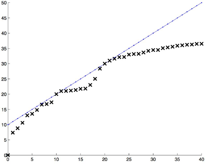
as can be proved via Laplace transforms. Now we define ‘time points’

$$t_{kn}\ :=\ \sum_{i=1}^{k}\theta_{in}^{2}\quad\text{and}\quad t_{kn}^{*}\ :=\ t_{j(n)n}+k-j(n)$$

with $j(n)$ any fixed index in $\mathcal{K}_{n}(\theta_{n})$. This construction entails that $t_{kn}^{*}\geq t_{kn}$ with equality if, and only if, $k\in\mathcal{K}_{n}(\theta_{n})$.

Figure 1 illustrates this construction. It shows the time points $t_{kn}$ (crosses) and $t_{kn}^{*}$ (dots and line) versus $k$ for a hypothetical signal $\theta_{n}\in\mathbb{R}^{40}$. Note that in this example, $\mathcal{K}_{n}(\theta_{n})$ is given by $\{10,11,20,21\}$.

Let $\Pi$, $G_{1}$, $G_{2}$, …, $G_{n}$, $Z_{1}$, $Z_{2}$, $Z_{3}$, …and $S^{2}$ be stochastically independent random variables, where $\Pi=(\Pi(t))_{t\geq 0}$ is a standard Poisson process, $G_{i}$ and $Z_{j}$ are standard Gaussian random variables, and $S^{2}\sim\chi_{m}^{2}$. Then one can easily verify that

$$\tilde{T}_{jkn} := \frac{m}{(k-j)S^{2}}\biggl{(}\,\sum_{i=j+1}^{k}G_{i}^{2}+\sum_{s=2\Pi(t_{jn}/2)+1}^{2\Pi(t_{kn}/2)}Z_{s}^{2}\biggr{)},$$

$$\tilde{T}_{jkn}^{*} := \frac{m}{(k-j)S^{2}}\biggl{(}\,\sum_{i=j+1}^{k}G_{i}^{2}+\sum_{s=2\Pi(t_{jn}^{*}/2)+1}^{2\Pi(t_{kn}^{*}/2)}Z_{s}^{2}\biggr{)}$$

define random variables $(\tilde{T}_{jkn})_{0\leq j<k\leq n}$ and $(\tilde{T}_{jkn}^{*})_{0\leq j<k\leq n}$ with the desired properties. $\Box$

Figure 1: Construction of the coupling

In the proofs of Theorems 3 and 4 we utilize repeatedly two elementary inequalities:

Lemma 7.

Let $a,b,c$ be nonnegative constants.

(i)  Suppose that $0\leq x\leq y\leq x+\sqrt{b(x+y)}+c$. Then

$$y\ \leq\ x+\sqrt{2bx}+b+\sqrt{bc}+c\ \leq\ x+\sqrt{2bx}+(3/2)(b+c).$$

(ii) For $x\geq 0$ define $h(x):=x+\sqrt{a+bx}+c$. Then

$$h(h(x))\ \leq\ x+2\sqrt{a+bx}+b/2+\sqrt{bc}+2c.$$

Proof of Lemma 7.

The inequality $y\leq x+\sqrt{b(x+y)}+c$ entails that either $y<x+c$ or

$$(y-x-c)^{2}\ \leq\ b(x+y)=2bx+b(y-x).$$

Since $y<x+c$ is stronger than the assertions of part (i), we only consider the displayed quadratic inequality. The latter is equivalent to

$$\bigl{(}y-x-(b/2+c)\bigr{)}^{2}\ \leq\ 2bx+(b/2+c)^{2}-c^{2}\ =\ 2bx+b^{2}/4+bc.$$

Hence the standard inequality $\sqrt{\sum_{i}z_{i}}\leq\sum_{i}\sqrt{z_{i}}$ for nonnegative numbers $z_{i}$ leads to

$$y-x\ \leq\ \sqrt{2bx}+\sqrt{b^{2}/4}+\sqrt{bc}+b/2+c\ =\ \sqrt{2bx}+b+\sqrt{bc}+c.$$

Finally, $0\leq\bigl{(}\sqrt{b}-\sqrt{c}\bigr{)}^{2}$ entails that $\sqrt{bc}\leq(b+c)/2$.

As to part (ii), the definition of $h(x)$ entails that

$$h(h(x)) = x+\sqrt{a+bx}+\sqrt{a+bx+b\sqrt{a+bx}+bc}+2c$$

$$\leq x+\sqrt{a+bx}+\sqrt{a+bx+b\sqrt{a+bx}}+\sqrt{bc}+2c$$

$$= x+\sqrt{a+bx}+\sqrt{a+bx}\sqrt{1+b/\sqrt{a+bx}}+\sqrt{bc}+2c$$

$$\leq x+2\sqrt{a+bx}+b/2+\sqrt{bc}+2c,$$

because $\sqrt{1+d}\leq 1+d/2$ for arbitrary $d\geq 0$. $\Box$

Proof of Theorem 3.

The definition of $\hat{\mathcal{K}}_{n,\alpha}$ and Proposition 2 together entail that $\hat{\mathcal{K}}_{n,\alpha}$ contains $\mathcal{K}_{n}(\theta_{n})$ with probability at least $1-\alpha$. The assertions about $\kappa_{n,\alpha}$ are immediate consequences of Theorem 1 applied to $\theta_{n}=\theta_{n}^{*}$.

Now we verify the oracle inequalities (10) and (11). Let $\gamma_{n}:=\bigl{(}4\|\theta_{n}\|^{2}+2n\big{)}^{1/2}\times\tau_{n}$. With $\gamma_{n}^{*}$ we denote the function $\gamma_{n}$ on $\mathcal{T}_{n}$ corresponding to $\theta_{n}^{*}$. Throughout this proof we use the shorthand notation $M_{n}(\ell,k):=M_{n}(\ell)-M_{n}(k)$ for $M_{n}=\hat{R}_{n},R_{n},\hat{L}_{n},L_{n}$ and arbitrary $\ell,k\in\mathcal{C}_{n}$. Furthermore, $\gamma_{n}^{(*)}(\ell,k):=\gamma_{n}^{(*)}(k,\ell)$ if $\ell>k$, and $\gamma_{n}^{(*)}(k,k):=0$.

In the subsequent arguments, $k_{n}:=\min(\mathcal{K}_{n}(\theta_{n}))$, while $j$ stands for a generic index in $\hat{\mathcal{K}}_{n,\alpha}$. The definition of the set $\hat{\mathcal{K}}_{n,\alpha}$ entails that

$$\hat{R}_{n}(j,k_{n})\ \leq\ \hat{\sigma}_{n}^{2}\Bigl{[}\gamma_{n}^{*}(j,k_{n})\Bigl{(}\Gamma\Bigl{(}\frac{j-k_{n}}{n}\Bigr{)}+\kappa_{n,\alpha}\Bigr{)}+O(\log n)\Bigr{]}.$$ (33)

Here and subsequently, $O(r_{n})$ and $O_{p}(r_{n})$ denote a generic number and random variable, respectively, depending on $n$ but neither on any other indices in $\mathcal{C}_{n}$ nor on $\alpha\in(0,1)$. Precisely, in view of our remark on dependence of $\alpha$, we consider all $\alpha\geq\alpha(n)$ with $\alpha(n)>0$ such that $\kappa_{n,\alpha(n)}=O(n^{1/6})$. Note that $\hat{\sigma}_{n}^{2}=1+O_{p}(n^{-1/2})$. Moreover, $\gamma_{n}^{*}(j,k_{n})^{2}\Gamma\bigl{(}(j-k_{n})/n\bigr{)}^{2}$ equals $12nx\log(e/x)\leq 12n$ with $x:=|j-k_{n}|/n\in[0,1]$. Thus we may rewrite (33) as

$$\hat{R}_{n}(j,k_{n})\ \leq\ \gamma_{n}^{*}(j,k_{n})\Bigl{(}\Gamma\Bigl{(}\frac{j-k_{n}}{n}\Bigr{)}+\kappa_{n,\alpha}\Bigr{)}+O_{p}(\log n).$$ (34)

Combining this with the equation $R_{n}(j,k_{n})=\hat{R}_{n}(j,k_{n})-\hat{D}_{n}(j,k_{n})$ yields

$$R_{n}(j,k_{n})\ \leq\ \gamma_{n}^{*}(j,k_{n})\Bigl{(}\Gamma\Bigl{(}\frac{j-k_{n}}{n}\Bigr{)}+\kappa_{n,\alpha}\Bigr{)}+O_{p}(\log n)+|\hat{D}_{n}(j,k_{n})|.$$ (35)

Since $\gamma_{n}^{*}(j,k_{n})^{2}\leq 6n$ and $\max_{t\in\mathcal{T}_{n}}|\hat{D}_{n}(t)|/\gamma_{n}(t)=O_{p}(\log n)$, (35) yields

$$R_{n}(j,k_{n})\ \leq\ \sqrt{12n}+\sqrt{6n}\,\kappa_{n,\alpha}+O_{p}(\log n)\gamma_{n}(j,k_{n}).$$

But elementary calculations yield

$$\gamma_{n}(j,k_{n})^{2}\ =\ \gamma_{n}^{*}(j,k_{n})^{2}+\mathop{\rm sign}(k_{n}-j)R_{n}(j,k_{n})\ \leq\ 6n+R_{n}(j,k_{n}).$$ (36)

Hence we may conclude that

$$R_{n}(j,k_{n})\ \leq\ O_{p}(\log n)\sqrt{R_{n}(j,k_{n})}+O_{p}\bigl{(}\sqrt{n}(\log n+\kappa_{n,\alpha})\bigr{)},$$

and Lemma 7 (i), applied to $x=0$ and $y=R_{n}(j,k_{n})$, yields

$$\max_{j\in\hat{\mathcal{K}}_{n,\alpha}}R_{n}(j,k_{n})\ \leq\ O_{p}\bigl{(}\sqrt{n}(\log n+\kappa_{n,\alpha})\bigr{)}.$$ (37)

This preliminary result allows us to restrict our attention to indices $j$ in a certain subset of $\mathcal{C}_{n}$: Since $0\leq R_{n}(n,k_{n})=n-k_{n}-\sum_{i=k_{n}+1}^{n}\theta_{in}^{2}$,

$$\sum_{i=k_{n}+1}^{n}\theta_{in}^{2}\ \leq\ n-k_{n}.$$

On the other hand, in case of $j<k_{n}$, $R_{n}(j,k_{n})=\sum_{i=j+1}^{k_{n}}\theta_{in}^{2}-(k_{n}-j)$, so

$$\sum_{i=j+1}^{n}\theta_{in}^{2}\ \leq\ n+O_{p}\bigl{(}\sqrt{n}(\log n+\kappa_{n,\alpha})\bigr{)}.$$

Thus if $j_{n}$ denotes the smallest index $j\in\mathcal{C}_{n}$ such that $\sum_{i=j+1}^{n}\theta_{in}^{2}\leq 2n$, then $k_{n}\geq j_{n}$, and $\hat{\mathcal{K}}_{n,\alpha}\subset\{j_{n},\ldots,n\}$ with asymptotic probability one, uniformly in $\alpha\geq\alpha(n)$. This allows us to restrict our attention to indices $j$ in $\{j_{n},\ldots,n\}\cap\hat{\mathcal{K}}_{n,\alpha}$. For any $\ell\geq j_{n}$, $\hat{D}_{n}(\ell,k_{n})$ involves only the restricted signal vector $(\theta_{in})_{i=j_{n}+1}^{n}$, and the proof of Theorem 1 entails that

$$\max_{j_{n}\leq\ell\leq n}\biggl{(}\frac{|\hat{D}_{n}(\ell,k_{n})|}{\gamma_{n}(\ell,k_{n})}-\sqrt{2\log n}-\frac{2c\log n}{\gamma_{n}(\ell,k_{n})}\biggr{)}^{+}\ =\ O_{p}(1).$$

Thus we may deduce from (35) the simpler statement that with asymptotic probability one,

$$R_{n}(j,k_{n}) \leq \bigl{(}\gamma_{n}^{*}(j,k_{n})+\gamma_{n}(j,k_{n})\bigr{)}\bigl{(}\sqrt{2\log n}+\kappa_{n,\alpha}+O_{p}(1)\bigr{)}$$

$$+\ O_{p}(\log n).$$

Now we need reasonable bounds for $\gamma_{n}^{*}(j,k_{n})^{2}$ in terms of $R_{n}(j)$ and the minimal risk $\rho_{n}=R_{n}(k_{n})$, where we start from the equation in (36): If $j<k_{n}$, then $\gamma_{n}(j,k_{n})^{2}=\gamma_{n}^{*}(j,k_{n})^{2}+4R_{n}(j,k_{n})$ and $\gamma_{n}^{*}(j,k_{n})^{2}=6(k_{n}-j)\leq 6\rho_{n}$. If $j>k_{n}$, then $\gamma_{n}^{*}(j,k_{n})^{2}=\gamma_{n}(j,k_{n})^{2}+4R_{n}(j,k_{n})$ and

$$\gamma_{n}(j,k_{n})^{2}=\sum_{i=k_{n}+1}^{j}(4\theta_{in}^{2}+2)\ \leq\ 4\rho_{n}+2R_{n}(j)\ =\ 6\rho_{n}+2R_{n}(j,k_{n}).$$

Thus

$$\gamma_{n}^{*}(j,k_{n})+\gamma_{n}(j,k_{n})\ \leq\ 2\sqrt{6}\sqrt{\rho_{n}}+\bigl{(}\sqrt{2}+\sqrt{6}\bigr{)}\sqrt{R_{n}(j,k_{n})},$$

and inequality (5.3) leads to

$$R_{n}(j,k_{n}) \leq \Bigl{(}4\sqrt{3}\sqrt{\log n}+2\sqrt{6}\,\kappa_{n,\alpha}+O_{p}(1)\Bigr{)}\sqrt{\rho_{n}}$$

$$+\ O_{p}\bigl{(}\sqrt{\log n}+\kappa_{n,\alpha}\bigr{)}\sqrt{R_{n}(j,k_{n})}+O_{p}(\log n)$$

for all $j\in\hat{\mathcal{K}}_{n,\alpha}$. Again we may employ Lemma 7 with $x=0$ and $y=R_{n}(j,k_{n})$ to conclude that

$$\max_{j\in\hat{\mathcal{K}}_{n,\alpha}}\,R_{n}(j,k_{n}) \leq \Bigl{(}4\sqrt{3}\sqrt{\log n}+2\sqrt{6}\,\kappa_{n,\alpha}+O_{p}(1)\Bigr{)}\sqrt{\rho_{n}}$$

$$+\ O_{p}\Bigl{(}(\log(n)^{3/4}+\kappa_{n,\alpha(n)}^{3/2})\rho_{n}^{1/4}+\log n+\kappa_{n,\alpha(n)}^{2}\Bigr{)}$$

uniformly in $\alpha\geq 0$.

If $\log(n)^{3}+\kappa_{n,\alpha(n)}^{6}=O(\rho_{n})$, then the previous bound for $R_{n}(j,k_{n})=R_{n}(j)-\rho_{n}$ reads

$$\max_{j\in\hat{\mathcal{K}}_{n,\alpha}}\,R_{n}(j)\ \leq\ \rho_{n}+\Bigl{(}4\sqrt{3}\sqrt{\log n}+2\sqrt{6}\,\kappa_{n,\alpha}+O_{p}(1)\Bigr{)}\sqrt{\rho_{n}}$$

uniformly in $\alpha\geq\alpha(n)$. On the other hand, if we consider just a fixed $\alpha>0$, then $\kappa_{n,\alpha}=O(1)$, and the previous considerations yield

$$\max_{j\in\hat{\mathcal{K}}_{n,\alpha}}\,R_{n}(j) \leq \rho_{n}+\bigl{(}4\sqrt{3}+o_{p}(1)\bigr{)}\sqrt{\log(n)\,\rho_{n}}$$

$$+\ O_{p}\bigl{(}\log(n)^{3/4}\rho_{n}^{1/4}+\log n\bigr{)}$$

$$\leq \rho_{n}+\bigl{(}4\sqrt{3}+o_{p}(1)\bigr{)}\sqrt{\log(n)\,\rho_{n}}+O_{p}(\log n).$$

To verify the latter step, note that for any fixed $\epsilon>0$,

$$\log(n)^{3/4}\rho_{n}^{1/4}\ \leq\ \begin{cases}\epsilon^{-1}\log n&\text{if}\ \rho_{n}\leq\epsilon^{-4}\log n,\\ \epsilon\sqrt{\log(n)\,\rho_{n}}&\text{if}\ \rho_{n}\geq\epsilon^{-4}\log n.\end{cases}$$

It remains to prove claim (11) about the losses. From now on, $j$ denotes a generic index in $\mathcal{C}_{n}$. Note first that

$$L_{n}(j,k_{n})-R_{n}(j,k_{n})\ =\ \sum_{i=j+1}^{k_{n}}(1-\epsilon_{in}^{2})\ =\ R_{n}(k_{n},j)-L_{n}(k_{n},j)\quad\text{if}\ j<k.$$

Thus Theorem 1, applied to $\theta_{n}=0$, shows that

$$\bigl{|}L_{n}(j,k_{n})-R_{n}(j,k_{n})\bigr{|}\ \leq\ \gamma_{n}^{+}(j,k_{n})\bigl{(}\sqrt{2\log n}+O_{p}(1)\bigr{)}+O_{p}(\log n),$$

where

$$\gamma_{n}^{+}(j,k_{n})\ :=\ \sqrt{2|k_{n}-j|}\ \leq\ \sqrt{2\rho_{n}}+\sqrt{2|R_{n}(j,k)|}.$$

It follows from $L_{n}(0)=R_{n}(0)=\|\theta_{n}\|^{2}$ that $L_{n}(j)-\rho_{n}$ equals

$$L_{n}(j,k_{n})+(L_{n}-R_{n})(k_{n},0)$$

$$= R_{n}(j,k_{n})+O_{p}\Bigl{(}\sqrt{\log(n)\rho_{n}}\Bigr{)}+O_{p}\bigl{(}\sqrt{\log n}\bigr{)}\sqrt{R_{n}(j,k_{n})}+O_{p}(\log n)$$

$$\geq O_{p}\Bigl{(}\sqrt{\log(n)\rho_{n}}+\log n\Bigr{)},$$

because $R_{n}(j,k_{n})\geq 0$ and $R_{n}(j,k_{n})+O_{p}(r_{n})\sqrt{R_{n}(j,k_{n})}\geq O_{p}(r_{n}^{2})$. Consequently, $\hat{\rho}_{n}:=\min_{j\in\mathcal{C}_{n}}L_{n}(j)$ satisfies the inequality

$$\hat{\rho}_{n}\ \geq\ \rho_{n}+O_{p}\Bigl{(}\sqrt{\log(n)\rho_{n}}+\log n\Bigr{)}\ =\ (1+o_{p}(1))\rho_{n}+O_{p}(\log n),$$

and this is easily shown to entail that

$$\rho_{n}\ \leq\ \hat{\rho}_{n}+O_{p}\bigl{(}\sqrt{\log n}\bigr{)}\sqrt{\hat{\rho}_{n}}+O_{p}(\log n)\ =\ (1+o_{p}(1))\hat{\rho}_{n}+O_{p}(\log n).$$

Now we restrict our attention to indices $j\in\hat{\mathcal{K}}_{n,\alpha}$ again. Here it follows from our result about the maximal risk over $\hat{\mathcal{K}}_{n,\alpha}$ that $L_{n}(j)-\rho_{n}$ equals

$$R_{n}(j,k_{n})+O_{p}\bigl{(}\sqrt{\log(n)\rho_{n}}\bigr{)}+O_{p}\bigl{(}\sqrt{\log n}\bigr{)}\sqrt{R_{n}(j,k_{n})}+O_{p}(\log n)$$

$$\leq 2R_{n}(j,k_{n})+O_{p}\bigl{(}\sqrt{\log(n)\rho_{n}}+\log n\bigr{)}\ \leq\ O_{p}\Bigl{(}\sqrt{\log(n)\rho_{n}}+\log n\Bigr{)}.$$

Hence $\max_{j\in\hat{\mathcal{K}}_{n,\alpha}}L_{n}(j)$ is not greater than

$$\rho_{n}+O_{p}\Bigl{(}\sqrt{\log(n)\rho_{n}}+\log n\Bigr{)}\ \leq\ \hat{\rho}_{n}+O_{p}\bigl{(}\sqrt{\log n}\bigr{)}\sqrt{\hat{\rho}_{n}}+O_{p}(\log n).$$

Proof of Theorem 4.

The application of inequality (19) in Corollary 6 to the tripel $(|J|,T_{n}(J)-|J|,\alpha/(2M_{n}))$ in place of $(n,\hat{\delta}^{2},\alpha)$ yields bounds for $\hat{\delta}_{n,\alpha,l}^{2}(J)$ and $\hat{\delta}_{n,\alpha,u}^{2}(J)$ in terms of $\hat{\delta}_{n}^{2}(J):=(T_{n}(J)-|J|)_{+}$. Then we apply (17-18) to $T_{n}(J)$, replacing $(n,\delta^{2},u)$ with $(|J|,\delta_{n}^{2}(J),\alpha^{\prime}/(2M_{n}))$ for any fixed $\alpha^{\prime}\in(0,1)$. By means of Lemma 7 (ii) we obtain finally

$$\left.\begin{array}[]{c}\hat{\delta}_{n,\alpha,u}^{2}(J)-\delta_{n}^{2}(J)\\ \delta_{n}^{2}(J)-\hat{\delta}_{n,\alpha,l}^{2}(J)\end{array}\right\} \leq (1+o_{p}(1))\sqrt{(16|J|+32\,\delta_{n}^{2}(J))\log M_{n}}$$

$$+\ (K+o_{p}(1))\log M_{n}$$

for all $J\in\mathcal{M}_{n}$. Here and throughout this proof, $K$ denotes a generic constant not depending on $n$. Its value may be different in different expressions. It follows from the definition of the confidence region $\hat{\mathcal{K}}_{n,\alpha}$ that for arbitrary $C\in\hat{\mathcal{K}}_{n,\alpha}$ and $D\in\mathcal{C}_{n}$,

$$R_{n}(C)-R_{n}(D) = \delta_{n}^{2}(D\setminus C)-\delta_{n}^{2}(C\setminus D)+|C|-|D|$$

$$= (\delta_{n}^{2}-\hat{\delta}_{n,\alpha,l}^{2})(D\setminus C)+(\hat{\delta}_{n,\alpha,u}^{2}-\delta_{n}^{2})(C\setminus D)$$

$$-\ \bigl{(}\hat{\delta}_{n,\alpha,u}^{2}(C\setminus D)-\hat{\delta}_{n,\alpha,l}^{2}(D\setminus C)+|D|-|C|\bigr{)}$$

$$\leq (\delta_{n}^{2}-\hat{\delta}_{n,\alpha,l}^{2})(D\setminus C)+(\hat{\delta}_{n,\alpha,u}^{2}-\delta_{n}^{2})(C\setminus D).$$

Moreover, according to (5.3) the latter bound is not larger than

$$(1+o_{p}(1))\Bigl{\{}\sqrt{\bigl{(}16|D\setminus C|+32\delta_{n}^{2}(D\setminus C)\bigr{)}\log M_{n}}$$

$$+\ \sqrt{\bigl{(}16|C\setminus D|+32\delta_{n}^{2}(C\setminus D)\bigr{)}\log M_{n}}\Big{\}}+(K+o_{p}(1))\log M_{n}$$

$$\leq (1+o_{p}(1))\sqrt{2\bigl{(}16|D|+32\delta_{n}^{2}(C^{\rm c})+16|C|+32\delta_{n}^{2}(D^{\rm c})\bigr{)}\log M_{n}}$$

$$\qquad\qquad\qquad\qquad\qquad\qquad+\ (K+o_{p}(1))\log M_{n}$$

$$\leq 8\sqrt{\bigl{(}R_{n}(C)+R_{n}(D)\bigr{)}\log M_{n}}\,(1+o_{p}(1))\ +\ (K+o_{p}(1))\log M_{n}.$$

Thus we obtain the quadratic inequality

$$R_{n}(C)-R_{n}(D) \leq 8\sqrt{\bigl{(}R_{n}(C)+R_{n}(D)\bigr{)}\log M_{n}}\,(1+o_{p}(1))$$

$$\qquad\qquad\qquad+\ (K+o_{p}(1))\log M_{n},$$

and with Lemma 7 this leads to

$$R_{n}(C)\ \leq\ R_{n}(D)+8\sqrt{2}\sqrt{R_{n}(D)\log M_{n}}(1+o_{p}(1))+(K+o_{p}(1))\log M_{n}.$$

This yields the assertion about the risks.

As for the losses, note that $L_{n}(\cdot)$ and $R_{n}(\cdot)$ are closely related in that

$$(L_{n}-R_{n})(D)\ =\ \sum_{i\in D}\epsilon_{in}^{2}-|J|$$

for arbitrary $D\in\mathcal{C}_{n}$. Hence we may utilize (17-18), replacing the tripel $(n,\delta^{2},u)$ with $(|D|,0,\alpha^{\prime}/(2\mu_{n}))$, to complement (5.3) with the following observation:

$$-A\sqrt{|D|\log M_{n}}\ \leq\ L_{n}(D)-R_{n}(D)\ \leq\ A\sqrt{|D|\log M_{n}}+A\log M_{n}$$ (42)

simultaneously for all $D\in\mathcal{C}_{n}$ with probability tending to one as $n\to\infty$ and $A\to\infty$. Note also that (42) implies that $R_{n}(D)\leq A\sqrt{R_{n}(D)\log M_{n}}+L_{n}(D)$. Hence

$$R_{n}(D)\ \leq\ (3/2)\bigl{(}L_{n}(D)+A^{2}\log M_{n}\bigr{)}\quad\text{for all}\ D\in\mathcal{C}_{n},$$

by Lemma 7 (i). Assuming that both (5.3) and (42) hold for some large but fixed $A$, we may conclude that for arbitrary $C\in\hat{\mathcal{K}}_{n,\alpha}$ and $D\in\mathcal{C}_{n}$,

$$L_{n}(C)-L_{n}(D)$$

$$= (L_{n}-R_{n})(C)-(L_{n}-R_{n})(D)+R_{n}(C)-R_{n}(D)$$

$$\leq A\sqrt{2(|C|+|D|)\log M_{n}}+A\sqrt{2\bigl{(}R_{n}(C)+R_{n}(D)\bigr{)}\log M_{n}}+4A\log M_{n}$$

$$\leq 2A\sqrt{2\bigl{(}R_{n}(C)+R_{n}(D)\bigr{)}\log M_{n}}+4A\log M_{n}$$

$$\leq A^{\prime}\sqrt{\bigl{(}L_{n}(C)+L_{n}(D)\bigr{)}\log M_{n}}+A^{\prime\prime}\log M_{n}$$

for constants $A^{\prime}$ and $A^{\prime\prime}$ depending on $A$. Again this inequality entails that

$$L_{n}(C)\ \leq\ L_{n}(D)+A^{\prime}\sqrt{2L_{n}(D)\log M_{n}}+A^{\prime\prime\prime}\log M_{n}$$

for another constant $A^{\prime\prime\prime}=A^{\prime\prime\prime}(A)$. $\Box$

6 Auxiliary results

This section collects some results from the vicinity of empirical process theory which are used in the present paper.

For any pseudo-metric space $(\mathcal{X},d)$ and $u>0$, we define the capacity number

$$\mathrm{D}(u,\mathcal{X},d)\ :=\ \max\bigl{\{}|\mathcal{X}_{o}|:\mathcal{X}_{o}\subset\mathcal{X},d(x,y)>u\ \text{for different}\ x,y\in\mathcal{X}_{o}\big{\}}.$$

It is well-known that convergence in distribution of random variables with values in a separable metric space may be metrized by the dual bounded Lipschitz distance. Now we adapt the latter distance for stochastic processes. Let $\ell_{\infty}(\mathcal{T})$ be the space of bounded functions $x:\mathcal{T}\to\mathbb{R}$, equipped with supremum norm $\|\cdot\|_{\infty}$. For two stochastic processes $X$ and $Y$ on $\mathcal{T}$ with bounded sample paths we define

$$d_{\rm w}(X,Y)\ :=\ \sup_{f\in\mathcal{H}(\mathcal{T})}\,\bigl{|}\mathbb{E}^{*}f(X)-\mathbb{E}^{*}f(Y)\bigr{|},$$

where $\mathbb{P}^{*}$ and $\mathbb{E}^{*}$ denote outer probabilities and expectations, respectively, while $\mathcal{H}(\mathcal{T})$ is the family of all funtionals $f:\ell_{\infty}(\mathcal{T})\to\mathbb{R}$ such that

$$|f(x)|\ \leq\ 1\quad\text{and}\quad|f(x)-f(y)|\ \leq\ \|x-y\|_{\infty}\quad\text{for all}\ x,y\in\ell_{\infty}(\mathcal{T}).$$

If $d$ is a pseudo-metric on $\mathcal{T}$, then the modulus of continuity $w(x,\delta\,|\,d)$ of a function $x\in l_{\infty}(\mathcal{T})$ is defined as

$$w(x,\delta\,|\,d):=\sup_{s,t\in\mathcal{T}:d(s,t)\leq\delta}\,|x(s)-x(t)|.$$

Furthermore, $\mathcal{C}_{u}(\mathcal{T},d)$ denotes the set of uniformly continuous functions on $(\mathcal{T},d)$, that is

$$\mathcal{C}_{u}(\mathcal{T},d)\ =\ \Big{\{}x\in l_{\infty}(\mathcal{T}):\lim_{\delta\searrow 0}w(x,\delta\,|\,d)=0\Big{\}}.$$

Theorem 8.

For $n=1,2,3,\ldots$ consider stochastic processes $X_{n}=\bigl{(}X_{n}(t)\bigr{)}_{t\in\mathcal{T}_{n}}$ and $Y_{n}=\bigl{(}Y_{n}(t)\bigr{)}_{t\in\mathcal{T}_{n}}$ on a metric space $(\mathcal{T}_{n},\rho_{n})$ with bounded sample paths. Then

$$d_{\rm w}(X_{n},Y_{n})\ \to\ 0$$

provided that the following three conditions are satisfied:

(i)  For arbitrary subsets $\mathcal{T}_{n,o}$ of $\mathcal{T}_{n}$ with $|\mathcal{T}_{n,o}|=O(1)$,

$$d_{\rm w}\Bigl{(}X_{n}\big{|}_{\mathcal{T}_{n,o}},Y_{n}\big{|}_{\mathcal{T}_{n,o}}\Bigr{)}\ \longrightarrow\ 0;$$

(ii)  for each number $\epsilon>0$,

$$\lim_{\delta\searrow 0}\underset{n\to\infty}{\lim\sup}\,\mathbb{P}^{*}\bigl{(}w(Z_{n},\delta\,|\,\rho_{n})>\epsilon\bigr{)}\ =\ 0\quad\text{for}\ Z_{n}=X_{n},Y_{n};$$

(iii)  for any $\delta>0$,  $\mathrm{D}(\delta,\mathcal{T}_{n},\rho_{n})=O(1)$.

Proof.

For any fixed number $\delta>0$ let $\mathcal{T}_{n,o}$ be a maximal subset of $\mathcal{T}_{n}$ such that $\rho_{n}(s,t)>\delta$ for differnt $s,t\in\mathcal{T}_{n,o}$. Then $|\mathcal{T}_{n,o}|=O(1)$ by Assumption (iii). Moreover, for any $t\in\mathcal{T}_{n}$ there exists a $t_{o}\in\mathcal{T}_{n,o}$ such that $\rho_{n}(t,t_{o})\leq\delta$. Hence there exists a partition of $\mathcal{T}_{n}$ into sets $B_{n}(t_{o})$, $t_{o}\in\mathcal{T}_{n,o}$, satisfying $t_{o}\in B_{n}(t_{o})\subset\bigl{\{}t\in\mathcal{T}_{n}:\rho_{n}(t,t_{o})\leq\delta\bigr{\}}$. For any function $x$ in $\ell_{\infty}(\mathcal{T}_{n})$ or $\ell_{\infty}(\mathcal{T}_{n,o})$ let $\pi_{n}x\in\ell_{\infty}(\mathcal{T}_{n})$ be given by

$$\pi_{n}x(t)\ :=\ \sum_{t_{o}\in\mathcal{T}_{n,o}}1\{t\in B_{n}(t_{o})\}x(t_{o}).$$

Then $\pi_{n}x$ is linear in $x\big{|}_{\mathcal{T}_{n,o}}$ with $\|\pi_{n}x\|_{\infty}=\bigl{\|}x\big{|}_{\mathcal{T}_{n,o}}\bigr{\|}_{\infty}$. Moreover, any $x\in\ell_{\infty}(\mathcal{T}_{n})$ satisfies the inequality $\|x-\pi_{n}x\|_{\infty}\leq w(x,\delta\,|\,\rho_{n})$. Hence for $Z_{n}=X_{n},Y_{n}$,

$$d_{\rm w}(Z_{n},\pi_{n}Z_{n}) \leq \sup_{h\in\mathcal{H}(\mathcal{T}_{n})}\mathbb{E}^{*}\bigl{|}h(Z_{n})-h(\pi_{n}Z_{n})\bigr{|}$$

$$\leq \mathbb{E}^{*}\min\bigl{(}\|Z_{n}-\pi_{n}Z_{n}\|_{\infty},1\bigr{)}$$

$$\leq \mathbb{E}^{*}\min\bigl{(}w(Z_{n},\delta\,|\,\rho_{n}),1\bigr{)},$$

and this is arbitrarily small for sufficiently small $\delta>0$ and sufficiently large $n$, according to Assumption (ii).

Furthermore, elementary considerations reveal that

$$d_{\rm w}(\pi_{n}X_{n},\pi_{n}Y_{n})\ =\ d_{\rm w}\Bigl{(}X_{n}\big{|}_{\mathcal{T}_{n,o}},Y_{n}\big{|}_{\mathcal{T}_{n,o}}\Bigr{)},$$

and the latter distance converges to zero, because of $|\mathcal{T}_{n,o}|=O(1)$ and Assumption (i).

Since

$$d_{\rm w}(X_{n},Y_{n})\ \leq\ d_{\rm w}(X_{n},\pi_{n}X_{n})+d_{\rm w}(Y_{n},\pi_{n}Y_{n})+d_{\rm w}(\pi_{n}X_{n},\pi_{n}Y_{n}),$$

these considerations entail the assertion that $d_{\rm w}(X_{n},Y_{n})\to 0$. $\Box$

Finally, the next lemma provides a useful inequality for $d_{\rm w}(\cdot,\cdot)$ in connection with sums of independent processes.

Lemma 9.

Let $X=X_{1}+X_{2}$ and $Y=Y_{1}+Y_{2}$ with independent random variables $X_{1}$, $X_{2}$ and independent random variables $Y_{1}$, $Y_{2}$, all taking values in $(\ell_{\infty}(\mathcal{T}),\|\cdot\|_{\infty})$. Then

$$d_{\rm w}(X,Y)\ \leq\ d_{\rm w}(X_{1},Y_{1})+d_{\rm w}(X_{2},Y_{2}).$$

For this lemma it is important that we consider random variables rather than just stochastic processes with bounded sample paths. Note that a stochastic process on $\mathcal{T}$ is automatically a random variable with values in $(\ell_{\infty}(\mathcal{T}),\|\cdot\|_{\infty})$ if (a) the index set $\mathcal{T}$ is finite, or (b) the process has uniformly continuous sample paths with respect to a pseudo-metric $d$ on $\mathcal{T}$ such that $N(u,\mathcal{T},d)<\infty$ for all $u>0$.

Proof of Lemma 9.

Without loss of generality let the four random variables $X_{1}$, $X_{2}$, $Y_{1}$ and $Y_{2}$ be defined on a common probability space and stochastically independent. Let $f$ be an arbitrary functional in $\mathcal{H}(\mathcal{T})$. Then it follows from Fubini’s theorem that

$$\bigl{|}\mathbb{E}f(X_{1}+X_{2})-\mathbb{E}f(Y_{1}+Y_{2})\bigr{|}$$

$$\leq \bigl{|}\mathbb{E}f(X_{1}+X_{2})-\mathbb{E}f(Y_{1}+X_{2})\bigr{|}+\bigl{|}\mathbb{E}f(Y_{1}+X_{2})-\mathbb{E}f(Y_{1}+Y_{2})\bigr{|}$$

$$\leq \mathbb{E}\,\Bigl{|}\mathbb{E}(f(X_{1}+X_{2})\,|\,X_{2})-\mathbb{E}(f(Y_{1}+X_{2})\,|\,X_{2})\Bigr{|}$$

$$+\ \mathbb{E}\,\Bigl{|}\mathbb{E}(f(Y_{1}+X_{2})\,|\,Y_{1})-\mathbb{E}(f(Y_{1}+Y_{2})\,|\,Y_{1})\Bigr{|}$$

$$\leq d_{\rm w}(X_{1},Y_{1})+d_{\rm w}(X_{2},Y_{2}).$$

The latter inequality follows from the fact that the functionals $x\mapsto f(x+X_{2})$ and $x\mapsto f(Y_{1}+x)$ belong to $\mathcal{H}(\mathcal{T})$, too. Thus $d_{\rm w}(X,Y)\leq d_{\rm w}(X_{1},Y_{1})+d_{\rm w}(X_{2},Y_{2})$. $\Box$

Acknowledgement.

Constructive comments of a referee are gratefully acknowledged.

References

- [1] Baraud, Y. (2004). Confidence balls in Gaussian regression. Ann. Statist. 32, 528-551.
- [2] Beran, R. (1996). Confidence sets centered at estimators. Ann. Inst. Statist. Math. 48, 1-15.
- [3] Beran, R. (2000). REACT scatterplot smoothers: superefficiency through basis economy. J. Amer. Statist. Assoc. 95, 155-169.
- [4] Beran, R. and Dümbgen, L. (1998). Modulation of estimators and confidence sets. Ann. Statist. 26, 1826-1856.
- [5] Birg, L. and Massart, P. (2001). Gaussian model selection. J. Eur. Math. Soc. 3, 203-268.
- [6] Cai, T.T. (1999). Adaptive wavelet estimation: a block thresholding and oracle inequality approach. Ann. Statist. 26, 1783-1799.
- [7] Cai, T.T. (2002). On block thresholding in wavelet regression: adaptivity, block size, and threshold level. Statistica Sinica 12, 1241-1273.
- [8] Cai, T.T. and Low, M.G. (2006). Adaptive confidence balls. Ann. Statist. 34, 202-228.
- [9] Cai, T.T. and Low, M.G. (2007). Adaptive estimation and confidence intervals for convex functions and monotone functions. Manuscript in preparation.
- [10] Dahlhaus, R. and Polonik, W. (2006). Nonparametric quasi-maximum likelihood estimation for Gaussian locally stationary processes. Ann. Statist. 34, 2790-2824.
- [11] Donoho, D.L. and Johnstone, I.M. (1994). Ideal spatial adaptation by wavelet shrinkage. Biometrika 81, 425-455.
- [12] Donoho, D.L. and Johnstone, I.M. (1995). Adapting to unknown smoothness via wavelet shrinkage. JASA 90, 1200-1224.
- [13] Donoho, D.L. and Johnstone, I.M. (1998). Minimax estimation via wavelet shrinkage. Ann. Statist. 26, 879-921.
- [14] Dümbgen, L. (2002). Application of local rank tests to nonparametric regression. J. Nonpar. Statist. 14, 511-537.
- [15] Dümbgen, L. (2003). Optimal confidence bands for shape-restricted curves. Bernoulli 9, 423-449.
- [16] Dümbgen, L. and Spokoiny, V.G. (2001). Multiscale testing of qualitative hypotheses. Ann. Statist. 29, 124-152.
- [17] Dümbgen, L. and Walther, G. (2007). Multiscale inference about a density. Technical report 56, IMSV, University of Bern.
- [18] Efromovich, S. (1998). Simultaneous sharp estimation of functions and their derivatives. Ann. Statist. 26, 273-278.
- [19] Futschik, A. (1999). Confidence regions for the set of global maximizers of nonparametrically estimated curves. J. Statist. Plann. Inf. 82, 237-250.
- [20] Genovese, C.R. and Wassermann, L. (2005). Confidence sets for nonparametric wavelet regression. Ann. Statist. 33, 698-729.
- [21] Hengartner, N.W. and Stark, P.B. (1995). Finite-sample confidence envelopes for shape-restricted densities. Ann. Statist. 23, 525-550.
- [22] Hoffmann, M. and Lepski, O. (2002). Random rates in anisotropic regression (with discussion). Ann. Statist. 30, 325-396.
- [23] Lepski, O.V., Mammen, E. and Spokoiny, V.G. (1997). Optimal spatial adaptation to inhomogeneous smoothness: an approach based on kernel estimates with variable bandwidth selectors. Ann. Statist. 25, 929-947.
- [24] Li, K.-C. (1989). Honest confidence regions for nonparametric regression. Ann. Statist. 17, 1001-1008.
- [25] Polyak, B.T. and Tsybakov, A.B. (1991). Asymptotic optimality of the -test for the orthogonal series estimation of regression. Theory Probab. Appl. 35, 293-306.
- [26] Robins, J. and van der Vaart, A. (2006). Adaptive nonparametric confidence sets. Ann. Statist. 34, 229-253.
- [27] Stone, C.J. (1984). An asymptotically optimal window selection rule for kernel density estimates. Ann. Statist. 12, 1285-1297.