How Gaussian competition leads to lumpy or uniform species distributions

Abstract

A central model in theoretical ecology considers the competition of a range of species for a broad spectrum of resources. Recent studies have shown that essentially two different outcomes are possible. Either the species surviving competition are more or less uniformly distributed over the resource spectrum, or their distribution is ’lumped’ (or ’clumped’), consisting of clusters of species with similar resource use that are separated by gaps in resource space. Which of these outcomes will occur crucially depends on the competition kernel, which reflects the shape of the resource utilization pattern of the competing species. Most models considered in the literature assume a Gaussian competition kernel. This is unfortunate, since predictions based on such a Gaussian assumption are not robust. In fact, Gaussian kernels are a border case scenario, and slight deviations from this function can lead to either uniform or lumped species distributions. Here we illustrate the non-robustness of the Gaussian assumption by simulating different implementations of the standard competition model with constant carrying capacity. In this scenario, lumped species distributions can come about by secondary ecological or evolutionary mechanisms or by details of the numerical implementation of the model. We analyze the origin of this sensitivity and discuss it in the context of recent applications of the model.

Introduction

A central model behind the theoretical description of competition among dissimilar species was introduced by MacArthur and Levins (1967). In the model, species are characterized by their niche position $x_{i}$, which measures a trait being relevant for the exploitation of a distributed resource. As examples, the niche value $x_{i}$ may represent body size of predators, where the distributed resource are preys with their size distribution, or $x_{i}$ could be beak sizes of birds, in which case the resource could be seeds of different sizes. Mathematically this leads to a Lotka-Volterra type of competition equation, where the competition coefficients are function of the distance between species on the niche axis $x$. This competition kernel is usually taken to be a Gaussian function of the niche difference (also called normal curve). The implication of this choice is the central topic of this paper.

The model was originally proposed as part of the hypothesis of limiting similarity, namely that competing species can coexist only if they are sufficiently different from each other (MacArthur and Levins, 1967; Abrams, 1983). A mathematical analysis of the model revealed that arbitrarily similar species could in fact coexist in some cases. However adding further effects to the model, like noise (May and MacArthur (1972), but see Turelli (1978)) or extinction thresholds (Pigolotti et al., 2007), impose a limit to the similarity between species. This sensitivity to second order effects has led to the conclusion that the model, in its original form, is structurally unstable when used to predict limits of similarity (Meszéna et al., 2006). The competition model has also been applied to describe coevolving species (MacArthur and Levins, 1967; Case, 1981) and used in some formulations of the theory of island biogeography (Roughgarden, 1979). More recently the same type of model has been simulated numerically and used as a basis for dynamical models of sympatric speciation (Doebeli and Dieckmann, 2000), food web assembly and evolution (Loeuille and Loreau, 2005; Johansson and Ripa, 2006; Lewis and Law, 2007), elucidating the relation between competition and predator-prey interactions (Chesson and Kuang, 2008), and for explaining lumped size distributions of species (Scheffer and van Nes, 2006). For a more extensive review of the biological applications and the generalization of the model see (Szabó and Meszéna, 2006). The competition model has been fundamental for the development of basic principles in theoretical ecology and it is relevant to achieve a full understanding of its technical aspects.

In almost all applications of the model the chosen competition kernel is Gaussian. This choice facilitates mathematical analysis, and was justified because the exact shape of the kernel was thought to have no influence on the fundamental results of the model. However, recent work has shown that the equilibrium solution can be one of two fundamentally different types, depending on the form of the competition kernel (Pigolotti et al., 2007). One class of competition kernels preserves all species initially introduced in the system, with adjustments only in their relative abundance. The final equilibrium is a state with species closely spaced and with roughly similar abundances (if the carrying capacity is also uniform). Another class of competition kernels leads to the species being lumped in dense groups (in some cases groups are formed by single species), separated by empty regions on the niche axis. Subsequent invasion of new species in these ‘exclusion zones’ is not possible due to competitive exclusion. The condition for uniform distribution of species is to have a positive definite competition kernel (see definition below). This criterion is automatically fulfilled when the kernel is constructed from the overlap of the species utilization of the resource (Roughgarden, 1979). If the kernel is not positive definite, a lumpy species distribution with exclusion zones emerges. The concern about this discovery is that, even though the Gaussian kernel is ecologically sound, it is exactly marginal between the two regimes. This indicates that numerical inaccuracies and/or secondary ecological effects may violate the positive definiteness of the competition kernel and cause a transition from a uniform to a lumpy species distribution.

The objective of this paper is to raise awareness in the theoretical ecology community of the potential pitfalls and subtleties associated with the use of Gaussian competition kernels or other marginal choices. To illustrate this, the consequences of the marginal nature of the Gaussian kernel in the competition model are explored, in the idealized case of a uniform carrying capacity. First, the sensitivity to ecologically relevant effects that may lead to lumpy distributions are examined. Then we examine the sensitivity to the details of numerical implementation. In the last section, we discuss the relevance of our results for the applications of the model.

Model

The competition model considers $n$ interacting populations, each utilizing a common distributed resource $x$ according to a utilization function $u_{i}(x)$, $i=1,...,n$. The dynamics of the abundance of species $i$, $N_{i}$, is described by a Lotka-Volterra set of competition equations:

$$\dot{N_{i}}=N_{i}\left(1-\frac{1}{K}\sum_{j=1}^{n}G_{ij}N_{j}\right),\ \ i=1,...,n,$$ (1)

where the growth rate (considered to be the same for all species) is set to one for simplicity, and the carrying capacity $K$ is uniform. Competition in (1) is described by competition coefficients $G_{ij}$ which are constructed from the overlap of utilization functions of competing species (MacArthur and Levins, 1967; Roughgarden, 1979):

$$G_{ij}=\frac{\int u_{i}(x)u_{j}(x)\,dx}{\int u_{i}^{2}(x)\,dx}.$$ (2)

A justification of (2) rests upon considering the probability that consumer $i$ meets consumer $j$ (Levins, 1968; Roughgarden, 1979).

Often, utilization functions are ignored, and the competition coefficients are postulated directly. It is usually assumed that species $i$ has an optimal exploitation of the resource at a value $x=x_{i}$, and the competition coefficients are taken to depend on the difference between the optimal resource values of two competing species, $y=|x_{i}-x_{j}|$, such that we can introduce the so-called competition kernel, $G_{ij}=G(y)$. Here we use a family of competition functions described by a parameter $p$:

$$G_{ij}=G(y)=e^{-|(x_{i}-x_{j})/\sigma|^{p}},$$ (3)

which contains the Gaussian kernel when $p=2$, or the exponential one when $p=1$. The width of the kernel $\sigma$ gives the range of competition on the niche axis. Incidentally the Gaussian kernel is obtained from Eq. (2) when the utilization functions are also Gaussian and of the form $u_{i}=\exp(-((x-x_{i})/s)^{2})$ with $s^{2}=\sigma^{2}/2$. When $p<2$ the kernels are more peaked around $y\approx 0$ and for $p>2$ they become more box-like (see Fig. 1).

Note that when competition coefficients are constructed by the formula (2), i.e. from the overlap of two utilization functions, they are always positive definite, meaning that $\sum_{ij}a_{i}G_{ij}a_{j}\geq 0$ for any set of numbers $a_{i}$ (Roughgarden, 1979) or, equivalently, that the Fourier transform of $G(y)$, defined as $\tilde{G}(k)=\int_{-\infty}^{+\infty}dx\ G(x)\exp(ikx)$, does not take negative values. This property holds for the family of kernels (3) for $p\leq 2$, but not for $p>2$ (Fig. 1). The Gaussian kernel is therefore marginal in the sense that, corresponding to the limit case $p=2$, even a very small perturbation may violate its positive definite character, generally believed to be an ecological requirement arising from expression (2).

An intuitive explanation for the appearance of the exclusion zones for $p>2$ is the following. Interaction kernels with large $p$ have a box-like shape. In these cases species compete very strongly with other species, roughly within a distance $\pm\sigma$ from their own niche value. Species with a niche $x$ in that range will therefore not be able to invade the resident species, leading to the exclusion zones between them. When $p$ is decreased, the resident species compete less and less with neighbouring species, until the exclusion zones disappear, leading to the possibility of continuous coexistence.

Understanding the fact that the transition occurs at $p=2$, and also the coexistence of more than one species in each cluster, requires a mathematical stability analysis of the model. Consider the uniform solution, in which many species having the same abundance are densely packed in niche space. Now perturb each population by a small quantity $\Delta N_{i}$, which can be either positive or negative. If the competition kernel is not positive defined, there are sets of perturbations such that $\sum\Delta N_{j}G_{ij}\Delta N_{i}$ is less than zero. One can show that such perturbations are amplified by the dynamics (Pigolotti et al., 2007), making the uniform solution unstable. The system will then evolve to a clustered state, where the distance between clusters is proportional to the interaction range $\sigma$.

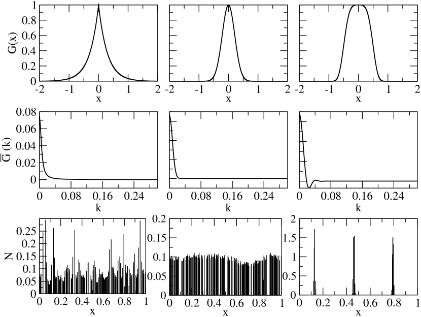
Figure 1: Three interaction kernels (top), their Fourier transform (middle row), and species distributions arising from simulation of the model after 1000 generations (bottom). Column are (Left) Exponential competition ($p=1$); (Center) Gaussian competition ($p=2$), and (Right) quartic competition ($p=4$). Simulations are initiated with $200$ species randomly distributed, $K=10$, and $\sigma=0.3$.

We mention here that a possible generalization is to consider multi-dimensional niche spaces. This possibility would complicate the mathematical notation but does not introduce qualitative changes. Stability in a multi-dimensional niche space still depends on the positive definiteness of the competition kernel. In particular, a multi-dimensional Gaussian competition kernel is still marginal in the sense described above.

We simulated the model (1) with competition kernel (3) for 1000 generations and $200$ species initially at random niche positions. The width of the kernel is $\sigma=0.3$ and the carrying capacity is $K=10$. The niche range is taken to be $x\in[0,1]$. The standard mathematical way to avoid effects due to the borders of the niche space is to adopt periodic boundary conditions (e.g. Scheffer and van Nes (2006)). These are introduced for mathematical convenience and aim at modeling species far from endpoints in a large niche space. Adopting periodic boundary conditions means that niche space is circular, so that when the interaction kernels extends beyond the left edge at $x=0$, it enters back into the right side at $x=1$ and vice versa. Periodic boundaries therefore mimic an infinite system by considering the niche segment $[0,1]$ as embedded in an array of repeated copies of itself. Mathematically, this is properly implemented by making a ’kernel wrap’, i.e. substitute $G(y)$ in (3) with $G_{p}(y)\equiv\sum_{n}G(y-n)$, where the sum runs from $n=0,\pm 1,\pm 2,...\pm\infty$. We call this implementation “fully periodic boundary conditions”, to distinguish it from another possibility considered below. Under fully periodic boundary conditions, the stability properties of the uniform solution are the same as in the infinite system.

Results

Simulations using the competition kernel (3) with $p=1$ (exponential), $2$ (Gaussian) and $4$ (box-like) illustrate the uniform species distributions for $p=1$ and $p=2$, and the lumped species clusters for $p=4$ (Fig. 1). The configurations in Fig. 1 are still transient states and, at longer times, configurations with $p\leq 2$ become more uniform, whereas the periodically spaced clusters of species for $p>2$ become thinner until they contain only a single species. In any case, from the initial stages until the final equilibrium, the main difference between the dynamics for the two classes of competition kernel is unchanged: for $p\leq 2$ all initial species are preserved, leading to dense and evenly distributed configurations, whereas ‘exclusion zones’ develop for $p>2$ leading to lumped species distributions.

Effects of secondary ecological processes

A natural question is whether the marginal nature of Gaussian competition can be brought on by secondary ecological effects. We have checked that adding a small immigration rate does not produce lumpy distributions. Adding noise or an extinction threshold (i.e. species are removed when their populations fall below a threshold) result in a limit to similarity between species, but does not lead to clustering (Pigolotti et al., 2007). This also happens in non marginal cases with $p<2$, where the minimum distance between species is unrelated to the competition range $\sigma$.

Effect of species extinction, invasion, and speciation was simulated by eliminating species below a given population threshold, and introducing invading species at a fixed rate. If they are introduced at random locations in niche space no patterns are observed. If invading species are introduced close to existing ones, modeling evolutionary change and speciation (Lawson and Jensen, 2007), the system ends with a lumped species distribution, even for $p=2$ (Fig. 2). However, the same mechanism has no effect if an exponential competition kernel ($p=1$) is chosen. The interpretation is that evolutionary effects favor the formation of lumpy species distributions, but only when the competition kernel is close to the Gaussian limiting case.

Figure 2: Final populations after $500\,000$ generations with speciation and extinction. Species whose population goes below $0.1$ are removed from the system. Every $100$ generations new species are introduced close to an existing one. The parent species is chosen with a probability proportional to its population; the distance of the new species to its parent is drawn from a Gaussian distribution of zero mean and spread $\sigma_{p}=0.02$. The new species $j$ is introduced with a population uniformly drawn from the interval $N\in[2,3]$. (Left panel) Gaussian kernel ($p=2$) and (Right panel) exponential kernel ($p=1$). Simulations are performed with fully periodic boundary conditions. $K=10$ and $\sigma=0.3$.

Effects due to truncation

The most obvious numerical simplification is to only partially implement the periodic boundary conditions, by omitting the kernel wrap around the niche interval, that is, using $G(y)$, with $y$ being the minimum of the two possible distances among species $i$ and $j$ ($|x_{i}-x_{j}|$ and $1-|x_{i}-x_{j}|$), instead of the periodic kernel $G_{p}(y)$. The resulting effective kernel is Gaussian but truncated at $|y|=1/2$, making it no longer positive definite. Although the shapes of $G(y)$ and $G_{p}(y)$ are still very similar for the parameters used here ($\sigma=0.3$), the change immediately leads to lumped species distributions (Fig. 3). In contrast, for $p=1$ (or any other values of $p<2$ which we have checked), changing $G_{p}(y)$ by $G(y)$ has no noticeable effect. Qualitatively, the dynamics for truncated Gaussian kernels resembles the outcome when the exponent of the competition kernel is perturbed just slightly. E.g. using $p=2.1$ instead of $p=2$ also leads to lumped species distributions, even when fully periodic boundary conditions are implemented (not shown).

While the mathematical analysis of “evolutionary diffusion” is rather complicated and results can be obtained only in the framework of simple models (Lawson and Jensen, 2007), the effect of truncation on the different kernels may be analyzed in more depth and is discussed in the next subsection.

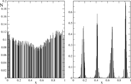
Figure 3: Populations of $200$ species after $1000$ generations with (left panel) Gaussian competition kernel with fully periodic boundary conditions, and (right panel) with truncated Gaussian competition kernel (see text). $K=10$ and $\sigma=0.3$.

Wavelength of Gaussian and exponential instabilities

We have numerically shown in the previous section that truncation leads to radically different results for the Gaussian and exponential kernel. This may be surprising when realizing that neither the truncated Gaussian nor the truncated exponential kernel are positive defined. The explanation of the different result comes from the wavelength of the modes $k$ for which the Fourier transform of the kernel $\tilde{G}(k)$ takes negative values, as it determines the distance between lumps (Pigolotti et al., 2007; Fort et al., 2009).

To find these wavelengths, we start from the Gaussian case and show what is the effect of truncating the kernel at a distance $a$ (which we take now to be the niche-space size, previously scaled to be 1) :

$$\tilde{G}_{p=2}(k)=\int_{-a}^{a}\exp(-x^{2}/\sigma^{2}-ikx)\ dx=\frac{\sqrt{\pi}\sigma}{2}e^{-\frac{k^{2}\sigma^{2}}{4}}\left[\mathrm{erf}\left(\frac{a}{\sigma}+\frac{ik\sigma}{2}\right)+c.c.\right],$$ (4)

where $\mathrm{erf}(x)=(2/\sqrt{\pi})\int_{0}^{x}\exp{-t^{2}}dt$ is the error function, and $c.c.$ stands for complex conjugate. We impose $a/\sigma\gg 1$, so we can get a simpler expression by expanding the error function, yielding

$$\tilde{G}_{p=2}(k)\approx\frac{\sqrt{\pi}\sigma}{2}\left[e^{-\frac{k^{2}\sigma^{2}}{4}}-2e^{-\frac{a^{2}}{\sigma^{2}}}\left(\frac{\sigma\cos(ka)}{\pi a}-\frac{2\sin(ka)}{\pi k\sigma}\right)\right]$$ (5)

From the previous expression we see that the wavenumbers that give negative modes are order $k\approx 2a/\sigma^{2}$.

We now check the same effect in the exponential case:

$$\tilde{G}_{p=1}(k)=\int_{-a}^{a}\exp(-|x|/\sigma-ikx)\ dx=\frac{2\sigma\left(1-e^{-\frac{a}{\sigma}}\cos(ak)+e^{-\frac{a}{\sigma}}k\sigma\sin(ak)\right)}{1+k^{2}\sigma^{2}}$$ (6)

In this case the instability occurs for large wavenumbers, proportional to $\exp(a/\sigma)$. We checked numerically that kernels with $p<2$ behave like the $p=1$ case, with the wavenumber of the first negative mode growing exponentially with the size of the niche space.

Summarizing, the kernels we considered develop an instability due to the truncation, but at very different frequencies: very high for the exponential kernel (exponential in the ratio between the system size and the kernel range) compared with the Gaussian (proportional to the same ratio). The consequence is that, already when the size of the niche space is large but not extremely large compared with the competition distance (like the cases considered here, $\sigma/a=0.3$), the unstable mode in the exponential case has a wavelength being much smaller than the interspecies distance, and is thus unable to generate patterns.

Discussion

The model (1)-(3) provides a very abstract representation of competition. Both empirical observations and theoretical approaches, based on explicit consideration of the coupled consumer-resource dynamics, lead to competition coefficients which are quite different from Gaussian (Schoener, 1974; Wilson, 1975; Ackermann and Doebeli, 2004), except in a few particular cases. Even so, the qualitative outcome of the model does not depend on the exact shape of the competition kernel, but only on its positive or non-positive definite character. We have restricted our considerations primarily to the basic model (1) with Gaussian interaction kernel and constant carrying capacity since it is the simplest implementation, allowing to illustrate in a clear setting the importance of $G$ and the issues caused by the choice of a marginal competition kernel.

The basic model with competition coefficients obtained from the overlap of utilization functions, which yields always positive definite kernels, allows for dense species distributions with no limits to similarity. This fundamental solution may be changed by three different effects: 1) effects stemming from the competition kernel being no longer positive definite lead to lumpy species distributions. Clusters of species will appear, separated by exclusion zones in niche space with a spacing proportional to the width of the competition kernel $\sigma$; 2) second order ecological effects like noise, species heterogeneity, evolutionary effects, or the introduction of an extinction threshold lead to a limit to the similarity with the spacing between species being independent of $\sigma$; 3) under a non constant carrying capacity, patterns of unevenly spaced species, lumpy or not, may appear. This lead Szabó and Meszéna (2006) to conclude that “the not-very-smooth nature of the carrying capacity seems to be essential for limiting similarity”. Notice that also some types of smooth, but non-uniform, carrying capacities may originate lumped distributions (Hernández-García et al., 2000)

The first case arises when the competition kernel is not positive definite. The main point of this paper is that, when the competition kernel is the marginal Gaussian, the model becomes very sensitive to additional effects that may lead to lumpy species distribution. As an example, we demonstrated that a simple representation of evolutionary diffusion (Lawson and Jensen, 2007) may lead to patterns in the Gaussian case. This effect is similar to that of evolutionary dynamics under assortative mating which shown to lead to lumpy species distributions (Doebeli et al., 2007). It is worth mentioning that, in the context of evolutionary dynamics, the fact that the presence of clusters depends of the choice of the competition kernel has been recently demonstrated (Leimar et al., 2008). Patterns can also result from numerical approximations, such as truncating the tails of a Gaussian competition kernel. This effect is probably the underlying mechanism behind species clustering observed in recent numerical work (Scheffer and van Nes, 2006), which was used to explain observed lumpy distributions (May et al., 2007). Additional ecological effects have been identified however (Scheffer and van Nes, 2006) which make the species groups a robust phenomenon (See Hernández-García et al. (2000) for analytical solutions of this type). In any case, these spurious effects can be avoided by paying attention to numerical details or by using a competition kernel which is not marginal, e.g. one with $p=1.5$, which in practice is almost indistinguishable from the Gaussian one. It is worth mentioning that analytical (i.e. not numerical) results are not affected by the marginal nature of the Gaussian kernel, both in relation to limiting similarity (May and MacArthur, 1972), coevolution (Case, 1981) or criteria for sympatric speciation (Doebeli and Dieckmann, 2000). The marginal nature of Gaussian competition kernel may however affect numerical work on food web evolution and assembly (Doebeli and Dieckmann, 2000; Loeuille and Loreau, 2005; Lewis and Law, 2007).

Since a non-positive definite competition kernel leads to lumpy species distributions a natural question is whether a non-positive definite kernel can result from hypothesis on ecological interactions. This case is often neglected in the literature, since assuming Eq. (2) automatically leads to a positive definite competition kernel (Roughgarden, 1979). However, as emphasized in Meszéna et al. (2006) and references therein, under quite general assumptions one should introduce two different utilization-like functions: a sensitivity function $S_{i}(x)$, describing the effect of the resource at $x$ on the growth of species $i$, and an impact function $D_{i}(x)$, describing the depletion of resources produced by $i$. Then, the competition coefficients depend on the overlap of these two quantities $\int S_{i}(x)D_{j}(x)dx$, and reduce to (2) only if the sensitivity and impact functions are proportional, with the constant of proportionality being the ecological efficiency. When the ecological efficiency is a function of $x$, and the sensitivity and impact functions are no longer proportional, the competition kernel may cease to be positive definite (Hernández-García et al., 2000).

The third mechanism is that of a non-constant carrying capacity $K(x)$, which has been explored by Szabó and Meszéna (2006). They found that some choices of carrying capacity leads to an irregular species lumping. The effect of non-constant carrying capacity in conjunction with both positive and non-positive definite competition kernels was explored by Hernández-García et al. (2000). The emerging picture is that the two mechanisms are independent. The cases in which a non-constant carrying capacity leads to uniform species distributions can also be destabilized by a non-positive definite kernel. This means that the mechanism explored here is not a particularity of constant carrying capacity but is present also in more general settings. It has been suggested that the effect of cutting the kernel is similar to that of having a finite niche space, i.e. of a box-like carrying capacity (Fort et al., 2009). However, this analogy does not hold to a rigorous mathematical analysis, which has demonstrated that lumps may appear when the carrying capacity is non-constant, but that this effect is not mathematically equivalent to a cut kernel (Hernández-García et al., 2000). Moreover, recent results (Baptestini et al., 2009) show how the effect of closed boundaries depend on the details of the boundary shape, so that the box-like case is not representative of a general finite niche space.

Having outlined the reasons that may cause the three different outcomes, the question arises if it is possible to infer whether one effect or the other is at play from the result of a numerical integration of the competition model. It can be difficult to distinguish between a uniform distribution of discrete species and a lumpy one when lumps are very narrow and close. Here, the fact that in the lumpy distribution the spacing of the lumps is proportional to the width of the competition kernel $\sigma$ can be used. If changing $\sigma$ results in a change in the distance between species proportional to $\sigma$, the effect is due to a non-positive definite competition kernel and vice versa. In the case where the effect is due to the carrying capacity being non-constant the spacing of species is usually more irregular (Szabó and Meszéna, 2006).

To summarize: in line with previous works we have found that the case of continuous coexistence (no limits to similarity) may be limited by a variety of effects, specially for the Gaussian kernel which has a marginal character. We have underlined that there are different ways to limit similarity, some leading to lumpy species distributions and others not. We hope that this article will increase the awareness in the theoretical ecological community of the potential subtleties associated with the use of the Gaussian competition kernel. Even though this functional form appears to be natural, in particular for analytical work, it may not be the most prudent choice for numerical exploration of the niche model.