Conductance and current noise of a superconductor/ferromagnet quantum point contact

Abstract

We study the conductance and current noise of a superconductor/ferromagnet ($S/F$) single channel Quantum Point Contact (QPC) as a function of the QPC bias voltage, using a scattering approach. We show that the Spin-Dependence of Interfacial Phase Shifts (SDIPS) acquired by electrons upon scattering by the QPC can strongly modify these signals. For a weakly transparent contact, the SDIPS induces sub-gap resonances in the conductance and differential Fano factor curves of the QPC. For high transparencies, these resonances are smoothed, but the shape of the signals remain extremely sensitive to the SDIPS. We show that noise measurements could help to gain more information on the device, e.g. in cases where the SDIPS modifies qualitatively the differential Fano factor of the QPC but not the conductance.

I Introduction

Mesoscopic circuits with ferromagnetic elements are generating a growing interest, both for the fundamentally new effects they can exhibit due to the lifting of spin-degeneracy, and for the possibilities of technological advances, e.g. towards nanospintronicsPrinz . The description of the interface between ferromagnetic and non-magnetic elements is crucial to understand the behavior of these devices. Obviously, one first has to take into account the spin-polarization of the electronic transmission probabilities through the interfaces, a property which generates the widely known magnetoresistance effectsMR . Importantly, the phases of the scattering amplitudes also depend on the spin in general. This so-called spin-dependence of interfacial phase shifts (SDIPS) is less frequently taken into account. However, the SDIPS has already been found to affect the behavior of many different types of mesoscopic conductors with ferromagnetic leads, like diffusive normal metal islands FNF , resonant systems CottetEurophys ; SST , Coulomb blockade systemsCB ; Cottet06 ; SST , or Luttinger liquidsLuttinger . The SDIPS can also have numerous types of consequences in superconducting/ferromagnetic ($S/F$) hybrid systems Tokuyasu ; otherBC ; AbsSpinValve ; cottet05 ; cottet06 ; Braude ; Zhao . It can e.g. produce effective field effects in superconducting electrodesTokuyasu ; AbsSpinValve ; cottet06 , or a phase shift of the spatial oscillations of the superconducting correlations induced by the proximity effect in a diffusive $F$ electrodecottet06 ; cottet05 . The SDIPS has also been predicted to induce triplet correlations in a $S$ electrode in contact with several ferromagnetic insulators with non-collinear polarization directionsBraude .

Recently, mean current measurements through $S/F$ quantum points contacts (QPCs) have raised much interest as a possible means to determine the polarization of a $F$ material. However, the effects of the SDIPS in these devices have not raised much attention so far. In most cases, the experimental results were interpreted in terms of a generalization of the Blonder-Tinkham-Klapwick (BTK) modelBTK to the spin-dependent case Soulen . We would like to emphasize that the description of a $S/F$ interface in terms of a delta-function barrier naturally includes a finite SDIPS but does not allow one to analyze its effects separately. Moreover, the SDIPS included in the generalized BTK model is specific for the delta-function barrier, and for a more realistic interface potential the SDIPS can be different. This is the reason why the influence of the transmission probabilities and of the SDIPS have to be investigated separately. The scattering approach seems perfectly adapted for this purpose since it allows to account explicitly for scattering phasesBlanter . In a few works, current transport through $S/F$ QPCs was described with a single-channel scattering descriptionPerezWillard ; Martin-Rodero . However, the SDIPS was not taken into account in these works.

In this article, we study how the conductance and the current noise through a single channel $S/F$ QPC are affected by the SDIPS, using a scattering approach. We would like to emphasize that the current noise in hybrid $S/F$ systems has draw little attention so farNoiseSF , although it can provide more information on the system considered. We find that the behavior of the QPC depends on its spin-dependent normal state transmission probabilities $T_{\sigma}$, but also on the difference $\Delta\varphi$ between the normal state reflection phases of up spins and down spins against $F$. The device is thus more difficult to characterize than in the spin-degenerate case since there are two more parameters to determine, i.e. $T_{\uparrow}-T_{\downarrow}$ and $\Delta\varphi$. We show that a finite SDIPS $\Delta\varphi\neq 0$ can strongly modify the behavior of the QPC, for instance by shifting the Andreev peaks appearing in the QPC conductance to subgap voltages, as found by Zhao et al. for $S/F/N$ quantum point contactsZhao , or by producing subgap peaks or dips in the differential Fano factor curves. At finite temperatures, we find that the SDIPS-induced shift of the Andreev peaks in the conductance can be difficult to distinguish from a gap reduction. We show that, in this context, a noise measurement can be very useful to characterize better the contact properties. This is particularly clear in cases where the QPC differential Fano factor versus bias voltage is qualitatively modified by the SDIPS while the conductance curve remains similar to the curves obtained without a SDIPS.

This paper is organized as follows: section II.A introduces expressions of the conductance and noise of a $S/F$ interface in the scattering formalism, section II.B presents an explicit expression of the scattering matrix of a single channel $S/F$ QPC, section II.C discusses the conductance and noise of this QPC at zero temperature, and section II.D discusses the finite temperature case. Section III concludes.

II Conductance and noise of a single channel $S/F$ QPC

II.1 Current and noise through a $S/F$ interface in the scattering approach

We consider a superconducting/ferromagnetic ($S/F$) interface with $S$ a conventional BCS conductor with a s-wave symmetry. We assume that the $S$ and $F$ leads can be considered as ballistic, so that the $S/F$ interface can be described with the scattering approachBlanter and the leads with Bogoliubov-De Gennes (BdG) equationsBdG . We use a gauge transformation to set the origin of the quasiparticles energies to the Fermi level of $S$, i.e. $\mu_{S}=0$Datta . Due to the bias voltage $V$ applied to the QPC, the Fermi level of $F$ is $\mu_{F}=-eV$, with $e=\left|e\right|$ the absolute value of the electron charge. In the following, we will denote by $(e,\sigma)$ electron states with spin $\sigma$ and by $(h,-\sigma)$ hole states in the $-\sigma$ spin band, with $\sigma\in\{\uparrow,\downarrow\}$ a spin component collinear to the polarization of $F$. A hole $(h,-\sigma)$ corresponding to an empty electronic state at an energy $-\varepsilon$ carries the same energy $\varepsilon$ as an electron $(e,\sigma)$ occupying a state with energy $\varepsilon$. These two types of quasiparticles are coupled by Andreev reflection processes occurring at the $S/F$ interface. One can thus write

$$b_{M,\alpha}(\varepsilon)=\sum\nolimits_{\gamma\in\mathcal{E}_{\sigma},Q\in\left\{F,S\right\}}\mathcal{S}_{M,Q}^{\alpha,\gamma}(\varepsilon)a_{Q,\gamma}(\varepsilon)$$

for $\alpha\in\mathcal{E}_{\sigma}$, with $\mathcal{E}_{\sigma}=\{(e,\sigma),(h,-\sigma)\}$ and $\mathcal{S}(\varepsilon)$ the scattering matrix of the $S/F$ interface for quasiparticles carrying an energy $\varepsilon$. Here, we consider the single channel case, so that $a_{M,\alpha}(\varepsilon)$ [$b_{M,\alpha}(\varepsilon)$] refers to the annihilation operator associated to the incident [outgoing] state for a particle with type $\alpha\in\mathcal{E}_{\sigma}$ and energy $\varepsilon$ of lead $M$. In the following, we use a picture consisting of both positive and negative energy states. The operator $\hat{I}(t)$ associated to the total current flowing through the device at time $t$ can be calculated as the sum of the electron and hole currents of the $\mathcal{E}_{\sigma}$ space, which replaces the summation on the spin directionDatta . More precisely, one has $\hat{I}(t)=\hat{I}_{e,\sigma}(t)+\hat{I}_{h,-\sigma}(t)$ with

$$\hat{I}_{\gamma}(t)=\frac{i\hbar e}{2m}\int dr_{\perp}\left\{\psi_{F,\gamma}^{\dagger}\left(\frac{\partial\psi_{F,\gamma}}{\partial z}\right)-\left(\frac{\partial\psi_{F,\gamma}^{\dagger}}{\partial z}\right)\psi_{F,\gamma}\right\}$$

for $\gamma\in\mathcal{E}_{\sigma}$. Here, $z$ is the coordinate along the leads and $r_{\perp}$ is the transverse coordinate. The field operator $\psi_{F,\gamma}$ associated with particles of type $\gamma$ in lead $F$ is defined as

$$\psi_{F,\gamma} =\int\limits_{-\infty}^{+\infty}d\varepsilon e^{-\frac{i\varepsilon t}{\hbar}}\frac{\chi_{F(r_{\perp})}}{\sqrt{2\pi v_{F}(\varepsilon)}}$$

$$\times(a_{F,\gamma}(\varepsilon)e^{i\lambda[\gamma]k_{F}(\varepsilon)z}+b_{F,\gamma}(\varepsilon)e^{-i\lambda[\gamma]k_{F}(\varepsilon)z})$$

with $\lambda[(e,\sigma)]=-1$, $\lambda[(h,-\sigma)]=+1.$ We have introduced above different quantities which characterize the conduction channel of the QPC, i.e. the transverse wave function $\chi_{F}$, the wavevector $k_{F}$, and the velocity of carriers $v_{F}=\hbar k_{F}/m$. The operator conjugated to $\psi_{F,\gamma}$ is denoted $\psi_{F,\gamma}^{\dagger}$. Neglecting the energy dependence of $v_{F}$ (see e.g. Ref. Blanter, ), one finds

$$\hat{I}_{\gamma}(t) =\frac{e}{h}\lambda[\gamma]\iint\limits_{-\infty,-\infty}^{+\infty,+\infty}d\varepsilon_{1}d\varepsilon_{2}e^{\frac{i(\varepsilon_{1}-\varepsilon_{2})t}{\hbar}}$$

$$\times\sum\limits_{\begin{subarray}{c}\alpha_{1},\alpha_{2}\\ M_{1},M_{2}\end{subarray}}a_{M_{1},\alpha_{1}}^{\dagger}(\varepsilon_{1})\mathcal{A}_{F,M_{1},M_{2}}^{\gamma,\alpha_{1},\alpha_{2}}(\varepsilon_{1},\varepsilon_{2})a_{M_{2},\alpha_{2}}(\varepsilon_{2})$$ (1)

with

$$\mathcal{A}_{F,M_{1},M_{2}}^{\gamma,\alpha_{1},\alpha_{2}}(\varepsilon_{1},\varepsilon_{2}) =\mathbb{I}_{F,\gamma}\delta_{M_{1},F}\delta_{M_{2},F}\delta_{\gamma,\alpha_{1}}\delta_{\gamma,\alpha_{2}}$$

$$-\left(\mathcal{S}_{F,M_{1}}^{\gamma,\alpha_{1}}(\varepsilon_{1})\right)^{{\dagger}}\mathcal{S}_{F,M_{2}}^{\gamma,\alpha_{2}}(\varepsilon_{2})$$ (2)

In the above Eqs., capital Latin indices correspond to the lead $F$ or $S$, Greek indices correspond to the electron or hole band of the space $\mathcal{E}_{\sigma}$, and $\mathbb{I}_{F,\gamma}$ is the identity matrix in the subspace of states of type $\gamma$ of lead $F$. In this paper, we study the average current $\left\langle I\right\rangle$ flowing through the interface and the zero-frequency current noise $S=2\int_{-\infty}^{+\infty}dt\left\langle\left[\hat{I}(t)-\langle I\rangle\right]\left[\hat{I}(0)-\langle I\rangle\right]\right\rangle$. Equations (1) and (2) lead to the expressions DeJong ; Anantram

$$\left\langle I\right\rangle=\frac{e}{h}\sum\limits_{M,\alpha,\gamma}\lambda(\alpha)\int\nolimits_{-\infty}^{+\infty}d\varepsilon f_{M}^{\gamma}(\varepsilon)\mathcal{A}_{F,M,M}^{\alpha,\gamma,\gamma}(\varepsilon,\varepsilon)$$ (3)

and

$$S(V) =\frac{2e^{2}}{h}\sum\limits_{M_{1},M_{2},\gamma_{1},\gamma_{2},\alpha,\beta}\lambda(\alpha)\lambda(\beta)$$

$$\times\int\nolimits_{-\infty}^{+\infty}d\varepsilon f_{M_{1}}^{\gamma_{1}}(\varepsilon)(1-f_{M_{2}}^{\gamma_{2}}(\varepsilon))\mathcal{A}_{F,M_{1},M_{2}}^{\alpha,\gamma_{1},\gamma_{2}}(\varepsilon,\varepsilon)\mathcal{A}_{F,M_{2},M_{1}}^{\beta,\gamma_{2},\gamma_{1}}(\varepsilon,\varepsilon)$$ (4)

We have introduced above the Fermi factors $f_{M}^{\gamma}(\varepsilon)=\left(1+\exp[\left(\varepsilon+\lambda[\gamma]\mu_{M}\right)/k_{B}T]\right)^{-1}$ with $T$ the temperature. In the limit $V\rightarrow 0$, Eqs. (3) and (4) fulfill the fluctuation dissipation theorem, i.e. $S=4k_{B}TG$ with $G(V)=\partial I/\partial V$.

In the limit $T=0$, simplified expressions of $G$ and $S$ can be obtained. In order to account for the two spin bands in the same way, we use a symmetry property stemming from the structure of the BdG equations, i.e. $\mathcal{T}_{M_{1},M_{2}}^{\alpha,\beta}(-\varepsilon)=\mathcal{T}_{M_{1},M_{2}}^{\widetilde{\alpha},\widetilde{\beta}}(\varepsilon)$, with $(\alpha,\beta)\in\mathcal{E}_{\sigma}^{2}$, $(M_{1},M_{2})\in\{S,F\}^{2}$, $\widetilde{(e,\sigma)}=(h,\sigma)$ and $\widetilde{(h,-\sigma)}=(e,-\sigma)$ (see derivation in Appendix A). Equations (3) and (4) combined with the unitarity of $\mathcal{S}(\varepsilon)$ then lead to

$$G\left(V\right)=\frac{e^{2}}{h}\sum\limits_{\sigma}\mathcal{W}_{F,F}^{(e,\sigma)}(\varepsilon=-eV)$$ (5)

with

$$\mathcal{W}_{F,F}^{(e,\sigma)}(\varepsilon)=\mathbb{I}_{F,(e,\sigma)}-\mathcal{T}_{F,F}^{(e,\sigma),(e,\sigma)}(\varepsilon)+\mathcal{T}_{F,F}^{(h,-\sigma),(e,\sigma)}(\varepsilon)$$ (6)

andcomp

$$S(V) =2\frac{e^{2}}{h}\sum\limits_{\sigma}\int\nolimits_{\mathcal{D}_{V}}d\varepsilon\left[2\mathcal{T}_{F,F}^{(h,-\sigma),(e,\sigma)}(\varepsilon)\mathcal{T}_{F,F}^{(e,\sigma),(e,\sigma)}(\varepsilon)\right.$$

$$+\mathcal{T}_{F,F}^{(e,\sigma),(e,\sigma)}(\varepsilon)\left(\mathbb{I}_{F,(e,\sigma)}-\mathcal{T}_{F,F}^{(e,\sigma),(e,\sigma)}(\varepsilon)\right)$$

$$\left.+\mathcal{T}_{F,F}^{(h,-\sigma),(e,\sigma)}(\varepsilon)\left(\mathbb{I}_{F,(h,-\sigma)}-\mathcal{T}_{F,F}^{(h,-\sigma),(e,\sigma)}(\varepsilon)\right)\right]$$ (7)

with $\mathcal{T}_{M_{1},M_{2}}^{\gamma_{1},\gamma_{2}}(\varepsilon)=\left|\mathcal{S}_{M_{1},M_{2}}^{\gamma_{1},\gamma_{2}}(\varepsilon)\right|^{2}$. Note that Eq. (5) is valid only if $\mathcal{W}_{F,F}^{\gamma}(\varepsilon)$, with $\gamma\in\mathcal{E}_{\sigma}$, can be considered as independent from $V$. The integration domain $\mathcal{D}_{V}$ in Eq.(7) is $[-e\left|V\right|,0]$ for $V>0$ and $[0,e\left|V\right|]$ for $V<0$, similarly to the fact that the elements $\mathcal{W}_{F,F}^{(e,\sigma)}$ contributing to $G\left(V\right)$ in Eq. (5) must be taken at $\varepsilon=\mp e\left|V\right|$ depending on the sign of $V$.

Before concluding this section, we note that in the multichannel case, the elements $\mathcal{S}_{M,Q}^{\alpha,\gamma}(\varepsilon)$ would be matrices relating the incoming and outgoing states of the different channels of leads $Q$ and $M$. In this case, one could generalize straightforwardly Eqs. (3), (4), (5) and (7) by applying to their right-hand sides a trace on the channels space and using $\mathcal{T}_{M_{1},M_{2}}^{\gamma_{1},\gamma_{2}}(\varepsilon)=\left(\mathcal{S}_{M_{1},M_{2}}^{\gamma_{1},\gamma_{2}}(\varepsilon)\right)^{{\dagger}}\mathcal{S}_{M_{1},M_{2}}^{\gamma_{1},\gamma_{2}}(\varepsilon)$. In section II, we focus on the single channel case. We briefly discuss possible extensions of this work to the multichannel case in section III.

II.2 Scattering matrix of a single channel $S/F$ QPC

We consider a $S/F$ interface which is narrow compared to the coherence length of $S$, so that it can be modeled as a specular $S/N$ interface in series with a (possibly) dirty $N/F$ interface, with the length of $N$ tending to zeroBeenakkerSNN . We would like to emphasize that the $N$ layer is introduced artificially, it is merely a trick to describe the superconducting interface on a scale much shorter that the coherence length. The matrix $\mathcal{S}(\varepsilon)$ of the $S/F$ interface can expressed in terms of the scattering matrix $\mathcal{P}^{\sigma}(\varepsilon)$ of electrons with spins $\sigma$ on the $N/F$ interface and of the amplitude $\gamma$ of the Andreev reflections at the $S/N$ interface. One finds in particular Xia ,

$$\mathcal{S}_{F,F}^{(e,\sigma),(e,\sigma)}(\varepsilon) =\mathcal{P}_{FF}^{\sigma}(\varepsilon)$$

$$+\gamma^{2}\mathcal{P}_{FN}^{\sigma}(\varepsilon)N^{\sigma}\left(\mathcal{P}_{NN}^{-\sigma}(-\varepsilon)\right)^{\ast}\mathcal{P}_{NF}^{\sigma}(\varepsilon)$$ (8)

$$\mathcal{S}_{F,F}^{(h,-\sigma),(e,\sigma)}(\varepsilon)=\gamma\left(\mathcal{P}_{FN}^{-\sigma}(-\varepsilon)\right)^{\ast}M^{\sigma}\mathcal{P}_{NF}^{\sigma}(\varepsilon)$$ (9)

$$M^{\sigma}=\left[\mathbb{I}_{N,(e,\sigma)}-\gamma^{2}\mathcal{P}_{NN}^{\sigma}(\varepsilon)\left(\mathcal{P}_{NN}^{-\sigma}(-\varepsilon)\right)^{\ast}\right]^{-1}$$ (10)

$$N^{\sigma}=\left[\mathbb{I}_{N,(h,-\sigma)}-\gamma^{2}\left(\mathcal{P}_{NN}^{-\sigma}(-\varepsilon)\right)^{\ast}\mathcal{P}_{NN}^{\sigma}(\varepsilon)\right]^{-1}$$ (11)

From Eqs. (5) and (7), at $T=0$, calculating the current and the noise through the $S/F$ interface only requires one to know the two elements of $\mathcal{S}(\varepsilon)$ given above. For $T\neq 0$, one must use Eqs. (3) and (4), so that the whole $S(\varepsilon)$ matrix is necessary (the other elements of $S(\varepsilon)$ are given in appendix B).

There remains to introduce explicit expressions for $\gamma$ and $\mathcal{P}^{\sigma}$. First, the amplitude $\gamma$ can be calculated using the ballistic BdG equations to model the $S/N$ interfaceBTK , with a step approximation for the gap $\Delta$ of $S$. This gives $\gamma=(\varepsilon-\mathrm{i}\sqrt{\Delta^{2}-\varepsilon^{2}})/\Delta$ for $\left|\varepsilon\right|<\Delta$ and $\gamma=(\varepsilon-\mathrm{sgn}(\varepsilon)\sqrt{\varepsilon^{2}-\Delta^{2}})/\Delta$ for $\left|\varepsilon\right|>\Delta$. Secondly, in the single channel case, the unitary of $\mathcal{P}^{\sigma}$ leads to

$$\mathcal{P}^{\sigma}=\left[\begin{tabular}[c]{ll}$\sqrt{R_{\sigma}}\exp\left[i\varphi_{FF}^{\sigma}\right]$&$\sqrt{T_{\sigma}}\exp\left[i\varphi_{FN}^{\sigma}\right]$\\ $\sqrt{T_{\sigma}}\exp\left[i\varphi_{NF}^{\sigma}\right]$&$\sqrt{R_{\sigma}}\exp\left[i\varphi_{NN}^{\sigma}\right]$\end{tabular}\ \ \ \ \right]$$

with $R_{\sigma}+T_{\sigma}=1$ and $\varphi_{NN}^{\sigma}+\varphi_{FF}^{\sigma}=\varphi_{NF}^{\sigma}+\varphi_{FN}^{\sigma}+\pi~{}[2\pi]$. In principle, the scattering phases $\varphi_{ij}^{\sigma}$, with $(i,j)\in\{N,F\}^{2}$, are spin-dependent because electrons are affected by a spin-dependent scattering potential at the $S/F$ interface. For simplicity, we will assume that $R_{\sigma}$, $T_{\sigma}$ and $\varphi_{ij}^{\sigma}$ are independent from $\varepsilon$ and $V$, which ensures the validity of Eq. (5) (see Ref. Vdrop, ). Note that the expression that we have introduced in this section for $\mathcal{S}$ implies $G(V)=G(-V)$ and $S(V)=S(-V)$, which is not a general property of superconducting hybrid devices (see e.g. Ref. Lesovik, ).

II.3 Conductance and noise of the QPC at zero-temperature

This section discusses the conductance and current noise of the single channel $S/F$ QPC at zero temperature ($T=0$). For $e\left|V\right|<\Delta$, no quasiparticle propagates in $S$, so that the unitarity of $\mathcal{S}(\varepsilon)$ leads to $\mathcal{T}_{F,F}^{(e,\sigma),(e,\sigma)}=1-\mathcal{T}_{F,F}^{(h,-\sigma),(e,\sigma)}$. One can thus calculate $G$ and $S$ from Eqs. (5) and (7) by using

$$\mathcal{T}_{F,F}^{(h,-\sigma),(e,\sigma)}(\varepsilon)$$

$$=\frac{T_{\uparrow}T_{\downarrow}}{1+R_{\uparrow}R_{\downarrow}-2\sqrt{R_{\uparrow}R_{\downarrow}}\cos[\varphi_{NN}^{\sigma}-\varphi_{NN}^{-\sigma}+2\varphi_{a}]}$$ (12)

for $\left|\varepsilon\right|<\Delta$, with $\varphi_{a}(\varepsilon)=\arg[\gamma]$. We note that in the absence of a SDIPS, i.e. $\varphi_{NN}^{\uparrow}=\varphi_{NN}^{\downarrow}$, Eq. (12) is in agreement with Eq. (7) of Ref. Martin-Rodero, . For $e\left|V\right|>\Delta$, one can calculate $G$ from Eq. (5) by using

$$\mathcal{W}_{F,F}^{(e,\sigma)}(\varepsilon)$$

$$=\frac{T_{\sigma}(1-\left|\gamma\right|^{2}R_{-\sigma})(1+\left|\gamma\right|^{2})}{1+\left|\gamma\right|^{4}R_{\uparrow}R_{\downarrow}-2\left|\gamma\right|^{2}\sqrt{R_{\uparrow}R_{\downarrow}}\cos[\varphi_{NN}^{\sigma}-\varphi_{NN}^{-\sigma}]}$$ (13)

for $\left|\varepsilon\right|>\Delta$. The expression of $S$ is too complicated to be given here. The above Eqs. describe a phenomenon analogous to the one predicted for a $S/F/N$ quantum point contactZhao . The denominators of Eqs. (12) and (13) contain interference terms which describe iterative reflection processes between the $S/N$ and $N/F$ interfaces (Andreev bound states). A quasiparticle can interfere with itself after two back and forth travels between $S$ and $F$, one as an electron $(e,\sigma)$ and one as a hole $(h,-\sigma)$. The conductance and noise depend on the phase difference $\Delta\varphi=\varphi_{NN}^{\uparrow}-\varphi_{NN}^{\downarrow}$ because the $N/F$ scattering matrix for holes is $\left(\mathcal{P}^{-\sigma}\right)^{\ast}$. This picture is in fact valid at any temperatures and voltages. In the general case, the whole $\mathcal{S}$ matrix is necessary to calculate the current and noise, but all the elements of $\mathcal{S}$ have the same denominator as the one appearing at the right hand side of Eq. (12) and (13) for $\left|\varepsilon\right|<\Delta$ and $\left|\varepsilon\right|>\Delta$ respectively [see Appendix B]. In addition, we have checked analytically that, in the general case, $G$ and $S$ depend on the phases of the $N/F$ scattering matrix through the parameter $\Delta\varphi$ only (they are actually periodic functions of $\Delta\varphi$ with a $2\pi$-periodicity).

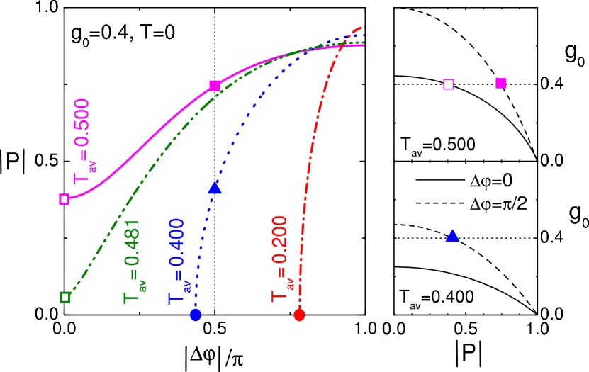
Figure 1: Left panel: Polarization $\left|P\right|$ calculated for $g_{0}=G(V=0)h/e^{2}=0.4$ and different values of $G(V=+\infty)=2T_{av}e^{2}/h$, as a function of the SDIPS parameter $\left|\Delta\varphi\right|$, at zero temperature ($T=0$). Right panels: Reduced zero-bias conductance $g_{0}$ of the QPC versus $\left|P\right|$, for $T_{av}=0.5$ (upper right panel), $T_{av}=0.4$ (bottom right panel) and different values of $\Delta\varphi$, i.e. $\Delta\varphi=0$ (solid lines) and $\Delta\varphi=\pi/2$ (dashed lines). In the left panel, $T_{av}\leq 0.5$ is assumed, so that the number of solutions for $\left|P\right|$ is either 0 or 1 depending on the value of $\left|\Delta\varphi\right|$. In all the cases considered, the inferred $\left|P\right|$ strongly increases with $\left|\Delta\varphi\right|$, because $g_{0}$ decreases with both $\left|P\right|$ and $-\left|\Delta\varphi\right|$ for $0<\left|\Delta\varphi\right|<\pi$ (see right panels). For high enough values of $T_{av}$,  there exists a $\left|P\right|$ solution for $\Delta\varphi=0$ (see e.g. open pink square for $T_{av}=0.5$ and open green square for $T_{av}=0.481$). For lower values of $T_{av}$ , there is no $\left|P\right|$ solution if $\Delta\varphi=0$, because the zero-bias conductance of the device cannot reach $g_{0}$ (see blue dotted line for $T_{av}=0.4$ and red dot-dashed line for $T_{av}=0.2$). However, it is possible to find a $\left|P\right|$ solution at $\left|\Delta\varphi\right|$ finite because $g_{0}$ increases with $\left|\Delta\varphi\right|$ for $0<\left|\Delta\varphi\right|<\pi$ (see e.g. blue triangle in the bottom right panel, for $T_{av}=0.4$ and $\left|\Delta\varphi\right|=\pi/2$). In some cases, a finite $\Delta\varphi$ can explain the considered values of $g_{0}$ and $T_{av}$ even in the absence of polarization (see blue and red solid circles in the left panel).

We now focus on the zero-voltage conductance $G(V=0)=g_{0}e^{2}/h$ of the QPC, which writes, from Eqs. (5) and (12),

$$g_{0}=\frac{4T_{\uparrow}T_{\downarrow}}{1+R_{\uparrow}R_{\downarrow}+2\sqrt{R_{\uparrow}R_{\downarrow}}\cos[\Delta\varphi]}\leq 4$$ (14)

In an experimental context, one may hope to determine the value of the polarization $P=(T_{\uparrow}-T_{\downarrow})/(T_{\uparrow}+T_{\downarrow})$ from the zero voltage conductance and the high voltage conductance $G(V=+\infty)=2T_{av}e^{2}/h$, with $T_{av}=\left(T_{\uparrow}+T_{\downarrow}\right)/2$. We define

$$A_{1(2)}=\left(g_{0}\cos(\Delta\varphi)\pm D\right)/\left(4-g_{0}\right)$$ (15)

with

$$D=\sqrt{16(1-2T_{av})+8g_{0}T_{av}-g_{0}^{2}\sin^{2}(\Delta\varphi)}~{}\text{.}$$ (16)

For $i\in\{1,2\}$, the polarizations $\pm P_{i}$ with

$$P_{i}=\frac{\sqrt{(1-T_{av})^{2}-A_{i}^{2}}}{T_{av}}$$ (17)

will be solutions of the problem provided $D$ is real and $0<A_{i}<1-T_{av}$. Thus, depending on the values of $T_{av}$, $g_{0}$ and $\Delta\varphi$, there can be either 0, 1 or 2 solutions for $\left|P\right|$. Importantly, the inferred values of $\left|P\right|$ depend not only on the zero voltage and normal conductances, but also strongly on $\Delta\varphi$. For simplicity, we will consider in the following the situation $T_{av}\leq 0.5$, for which one has $A_{1}>0$ and $A_{2}<0$, so that there is either no solution for $\left|P\right|$ or one solution $\left|P\right|=\left|P_{1}\right|$ if $A_{1}<1-T_{av}$. This situation is illustrated in Fig. 1, whose left panel shows the calculated $\left|P\right|$ as a function of $\left|\Delta\varphi\right|$ for $g_{0}=0.4$ and different values of $T_{av}$, with $T_{av}\leq 0.5$ (the use of $\left|\Delta\varphi\right|$ is due to the fact that $\left|P\right|$ is an even function of $\Delta\varphi$). For the largest values of $T_{av}$ used in Fig. 1, left panel (see pink solid curve and green double dot-dashed curve), a finite $\left|P\right|$ is found for $\Delta\varphi=0$ (see pink and green open squares). However, the calculated $\left|P\right|$ can also be larger if one uses a finite $\left|\Delta\varphi\right|$. This can be understood by noting that, for the relatively low values of $T_{av}$ used in this Figure and $0<\left|\Delta\varphi\right|<\pi$, $g_{0}$ decreases monotonically with both $\left|P\right|$ and $-\left|\Delta\varphi\right|$. An increase in $\left|\Delta\varphi\right|$ thus compensates an increase in $\left|P\right|$ (see upper right panel of Fig. 1). For the lowest values of $T_{av}$ used in Fig. 1, left panel (see blue dotted curve and red dot-dashed curve), there is no $\left|P\right|$ solution if $\Delta\varphi=0$, because the zero-bias conductance of the device cannot reach the considered value $g_{0}=0.4$. However, as long as $g_{0}$ is not too large, it is possible to find a $\left|P\right|$ solution at $\left|\Delta\varphi\right|$ finite because the zero bias conductance of the QPC increases with $\left|\Delta\varphi\right|$ for $0<\left|\Delta\varphi\right|<\pi$ (see e.g. blue triangle in the bottom right panel of Fig. 1). In this case, the calculated value of $\left|P\right|$ also increases with $\left|\Delta\varphi\right|$, for the same reason as previously. Note that due to the continuity of the equations, there exists a limiting case where a finite $\Delta\varphi$ can explain the considered values of $g_{0}$ and $T_{av}$ in absence of polarization (these points are indicated with solid circles in Fig. 1)note2 . For $T_{av}\geq 0.5$, $g_{0}$ is not always a monotonic function of $\left|P\right|$, so that there can be 2 solutions $\left|P_{1}\right|$ and $\left|P_{2}\right|$ for $\left|P\right|$ in some situations (not shown). We conclude that even in the single-channel case, knowing the zero and high voltage conductances of the QPC is not sufficient to determine $P$note . We will thus consider below the full voltage dependence of $G(V)$, which brings more information on the system. We will also show that noise measurements prove to be very useful to characterize unambiguously the properties of the QPC.

The top panels of Figs. 2 and 3 show the voltage dependence of $G$ for low and high values of $T_{av}$, respectively. In this paragraph, we comment on the results for $T=0$ only (black full lines). For $\Delta\varphi=0$, the conductance shows peaks at $eV=\pm\Delta$, because for $\varepsilon=\pm\Delta$, one has $2\varphi_{a}=0$ [$2\pi$], so that the multiple reflection paths between $S$ and $F$ interfere constructively. Between these peaks, the conductance reaches a minimum of $4(e^{2}/\hbar)T_{\uparrow}T_{\downarrow}/[1+(R_{\uparrow}R_{\downarrow})^{1/2}]^{2}$ at $V=0$. The existence of a finite SDIPS can strongly modify this behavior. Indeed, for $\Delta\varphi\neq 0$ and a small enough value of $T_{av}$, the resonance peaks of $G(V)$ are shifted to lower voltages $V=\pm V_{p}$ with $eV_{p}\simeq\Delta\cos(\Delta\varphi/2)<\Delta$ (Fig. 2, top middle panel). For $\Delta\varphi=\pi$, these peaks are merged into a single peak and $G(V)$ is maximum at $V=0$ (Fig. 2, top right panel). For high values of $T_{av}$, no clear subgap conductance peaks occur, but the curvature of the sub-gap $G(V)$ characteristic can be inverted by a finite SDIPS (Fig. 3, top panels). The $G(V)$ curve is independent from $\Delta\varphi$ only if interferences are suppressed for one spin direction, i.e. $T_{\uparrow}=1$ or $T_{\downarrow}=1$. Above the gap, in any case, the conductance of the device drops to its normal-state value $2\left(e^{2}/h\right)T_{av}$ which does not depend on the SDIPS.

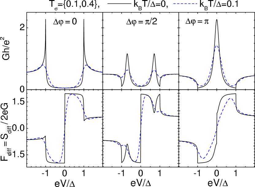
Figure 2: Conductance $G$ (top panels) and differential Fano factor $F_{diff}=(dS/dV)/2eG$ (bottom panels) as a function of the bias voltage $V$ for $T_{\uparrow}=0.4,T_{\downarrow}=0.1$, different temperatures (black solid lines $T=0$, blue dashed lines $k_{B}T/\Delta=0.1$), and different values of $\Delta\varphi$ (left panels: $\Delta\varphi=0$, middle panels $\Delta\varphi=\pi/2$, right panels $\Delta\varphi=\pi$).

The current noise through the $S/F$ QPC can provide more information on its properties, which is of particular interest since this device is characterized by a larger number of parameters than in the spin-degenerate case. According to Eqs. (5) and (7), the conductance and the noise are not mathematically equivalent and the noise can thus provide information complementary to the conductance. The bottom panels of Figure 2 and 3 show the voltage dependence of the differential Fano factor $F_{diff}=(dS(V)/dV)/2eG$ for low and high values of $T_{av}$, respectively. This quantity can be measured directly (see e.g. Ref. Schoelkopf, ) or obtained from a $S(V)$ measurement. In this paragraph, we comment on the results for $T=0$ only. One can first note that $F_{diff}(V)$ is an odd function of $V$ due to $S(V)=S(-V)$. For a low $T_{av}$ and $\Delta\varphi=0$, $F_{diff}$ shows subgap plateaus at values $\pm 2[(r_{\uparrow}+r_{\downarrow})/(1+r_{\uparrow}r_{\downarrow})]^{2}$ for $V\gtrless 0$, with $r_{\sigma}=(R_{\sigma})^{1/2}$. For $\Delta\varphi\neq 0$, a dip/peak appears on these plateaus, at the resonance voltages $V=\pm V_{p}$, again due to constructive quasiparticle interferences (Fig. 2, bottom middle panel). For higher values of $T_{av}$, the dips and peaks are smoothed, but the shape of $F_{diff}(V)$ remains sensitive to $\varphi$ as long as $T_{\uparrow}T_{\downarrow}<1$ (Fig. 3). Above the gap, in any case, $F_{diff}$ drops to the normal state value $(\sum\nolimits_{\sigma}T_{\sigma}[1-T_{\sigma}])/(\sum\nolimits_{\sigma}T_{\sigma})$ which does not depend on the SDIPS. One can thus determine the polarization $P$ of the tunnel rates by using

$$P^{2}=\frac{2e^{2}}{h}\frac{1-F_{diff}(V=+\infty)}{G(V=+\infty)}-1$$

Then, the SDIPS parameter $\Delta\varphi$ and the BCS gap $\Delta$ can be determined from the voltage dependence of the conductance and noise curves.

II.4 Conductance and noise of the QPC at finite temperatures

We now comment on the finite temperature $G(V)$ and $F_{diff}(V)$ curves, obtained by differentiating Eqs. (3) and (4) with respect to $V$ (see blue dashed lines in Figs. 2 and 3). At first glance, these curves simply seem to be thermally rounded. However, the finite temperature expressions of $G(V)$ and $F_{diff}(V)$ involve elements of the $\mathcal{S}$ matrix which do not appear in the zero-temperature expressions, thus the finite temperature curves sometimes display features not predictable from the zero temperature curves. For instance, in the bottom left panel of Fig. 3, a slight dip[peak] appears in the $F_{diff}(V)$ curve at $V=[-]\Delta/e$ for $T\neq 0$, an effect not present for $T=0$.

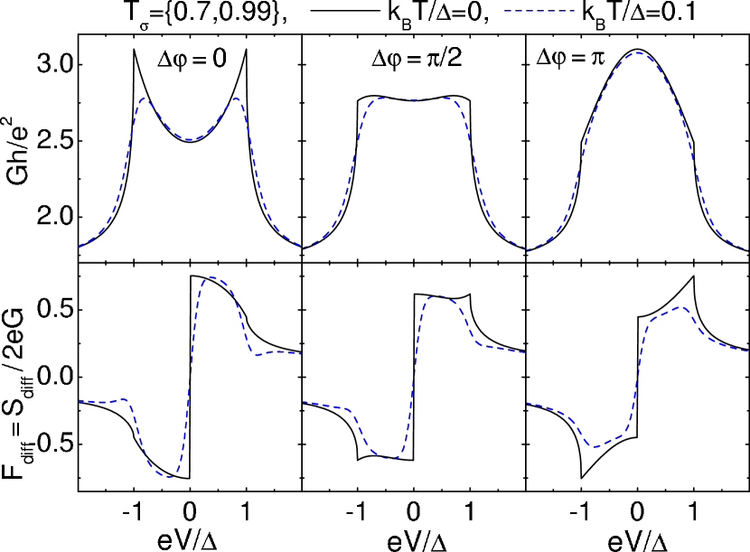
Figure 3: Conductance $G$ (top panels) and differential Fano factor $F_{diff}$ (bottom panels) as a function of the bias voltage $V$ for $T_{\uparrow}=0.99,T_{\downarrow}=0.7$, different temperatures (black solid lines $T=0$, blue dashed lines $k_{B}T/\Delta=0.1$), and different values of $\Delta\varphi$ (left panels: $\Delta\varphi=0$, middle panels $\Delta\varphi=\pi/2$, right panels $\Delta\varphi=\pi$).

In the case of a weakly transparent contact, since the Andreev resonance peaks of the conductance are shifted to lower voltages for $\Delta\varphi\neq 0$, one can obtain, for $T\neq 0$, conductance curves similar to those obtained for $\Delta\varphi=0$ and a reduced value of $\Delta$. The determination of the quantum point contact properties from the $G(V)$ curves alone can thus be difficult at finite temperatures. Figure 4 shows two examples where measuring the voltage dependence of the noise can clearly bring more information on the system. The left panel presents two cases where the $G(V)$ curves are extremely close, one case with $\Delta\varphi\neq 0$ and one case with $\Delta\varphi=0$ and a reduced gap value. The corresponding $F_{diff}(V)$ curves have a strong quantitative difference, which can help to discriminate the two cases. The right panels of Fig. 4 present two cases where the $G(V)$ curves are qualitatively similar, one case with $\Delta\varphi\neq 0$ and one case with $\Delta\varphi=0$ and a reduced gap value. The corresponding $F_{diff}(V)$ curves have a strong qualitative difference, which can help to discriminate the two cases again. In the case $\Delta\varphi\neq 0$, the differential Fano factor shows a secondary peak[dip] at $eV>0$ [ $eV<0$]. This effect, which can also be seen in the bottom middle panel of Fig. 2, never occurs for $\Delta\varphi=0$.

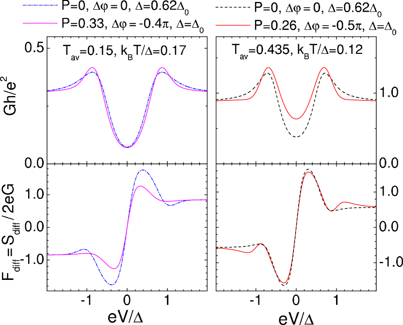
Figure 4: Conductance $G$ (top panels) and differential Fano factor $F_{diff}$ (bottom panels) as a function of the bias voltage $V$, for different sets of parameters. The left panels compare a case with a finite SDIPS (pink solid lines) and a case with no SDIPS and a smaller gap value $\Delta$ (blue dash-dotted lines). The conductance curves obtained in the two cases (top left panels) are very close, but the differential Fano factor curves (bottom left panels) have a strong quantitative difference. The right panels also compare a case with a finite SDIPS (red solid lines) and a case with no SDIPS and a smaller $\Delta$ (black dashed lines). In these two cases, the conductance curves (top right panel) are qualitatively similar but the Fano factor curves (bottom right panel) show a strong qualitative difference: in the case of a finite SDIPS, $F_{diff}(V)$ shows a secondary peak[dip] at $eV>\Delta$ [$eV<\Delta$]. This feature never appears in the absence of a SDIPS. Note that the high voltage limits of the two $F_{diff}(V)$ curves shown in the bottom left (bottom right) panel are different, but that this difference is not visible on the scale shown in the figure.

Before concluding this section, we point out that in most cases, experimental results on $S/F$ QPCs were interpreted with various models inspired from the BTK approachSoulen . The effect of the SDIPS was not studied in these works. However the description of a $S/F$ interface with a delta-function barrier naturally takes into account the SDIPS. We have checked that the spin-dependent BTK-like model corresponds to a particular case of the scattering model of Sec. II (generalized to the multichannel case), with parameters given in appendix C.

III Conclusion and discussion

In this paper, we have studied the conductance $G$ and noise $S$ of a superconducting/ferromagnetic ($S/F$) single channel Quantum Point Contact (QPC) as a function of the QPC bias voltage $V$, using a scattering approach. We have shown that the Spin-Dependence of Interfacial Phase Shifts (SDIPS) acquired by electrons at the $S/F$ interface strongly modifies these signals. In particular, for a weakly transparent contact, the SDIPS produces unusual sub-gap resonances or dips in the $G(V)$ and $S(V)$ curves. We have shown that measuring the noise should help to gain information on the system. This fact is well illustrated e.g. by cases where the SDIPS modifies qualitatively the zero-frequency noise but not the conductance.

One should note that, so far, experiments on $S/F$ quantum point contacts were performed in the multichannel limit. Although single-channel contacts were already realized in the $S/N$ caseScheer , this seems more difficult in the $S/F$ case with the present fabrication techniques. A multichannel theory should thus be very useful. For a multichannel disordered $S/N$ QPC, Ref. BeenakkerSNN, has shown that, due to time reversal symmetry, the eigenstates the QPC normal state scattering matrix are also those of $\mathcal{S}$. As a consequence, the multichannel generalization of $G(V)$ and $S(V)$ just requires a summation on the normal channels index. In the $S/F$ case, the calculation should be more complicated because time reversal symmetry breaking suppresses the normal channels independence Martin-Rodero ; Xia . So far, the multichannel case has been addressed with the BTK model, in which the hypothesis of a specular interface allows one to consider the normal channels as independent in spite of the time reversal symmetry breakingDeJong ; Zutic . However, this approach lacks of generality since it imposes a particular relation between the transmission probabilities and the SDIPS parameters, and it is not valid for disordered interfaces. Interestingly, Refs. Xia, reports on the ab-initio modelization of a particular type of disordered multichannel $S/F$ interface. However, to our knowledge, the multichannel $S/F$ case has not been studied with a more general approach so far. Our work suggests that such a study should take into account the SDIPS. Considering that, even in the single channel case, the conductance and noise of the device vary nonlinearly with the SDIPS parameter (see e.g. Eq. 12), there is no reason to expect that the effects of the SDIPS average out in the multichannel case, even in the extreme case of a SDIPS parameter $\Delta\varphi^{n}$ randomly distributed with the channel index $n$.

We would like to acknowledge useful discussions with C. Bruder, B. Douçot and T. Kontos. This work was financially supported by the Swiss National Science Foundation, the DFG through SFB 513 and SFB 767, the Priority Programm Semiconductor Spintronics, and the Landesstiftung Baden-Württemberg through the Kompetenznetzwerk Funktionelle Nanostrukturen.

IV Appendix A : A symmetry property of the scattering matrix $\mathcal{S}$

This appendix shows that the property $\mathcal{T}_{M_{1},M_{2}}^{\alpha,\beta}(-\varepsilon)=\mathcal{T}_{M_{1},M_{2}}^{\widetilde{\alpha},\widetilde{\beta}}(\varepsilon)$, with $(\alpha,\beta)\in\mathcal{E}_{\sigma}^{2}$ and $(M_{1},M_{2})\in\{S,F\}^{2}$, used to derive Eqs. (5) and (7) is a general property which stems from the symmetries of the BdG equations.

We first consider the eigenstates of the BdG equations in a bulk S. An eigenstate with energy $\varepsilon$ in the subspace $\mathcal{E}_{\sigma}=\{(e,\sigma),(h,-\sigma)\}$ has electron and hole components $u_{\sigma}$ and $v_{-\sigma}$ such that

$$\left[\begin{array}[c]{cc}H_{\sigma}&\Delta\\ \Delta^{\ast}&-H_{-\sigma}^{\ast}\end{array}\right]\left[\begin{array}[c]{c}u_{\sigma}\\ v_{-\sigma}\end{array}\right]=\varepsilon\left[\begin{array}[c]{c}u_{\sigma}\\ v_{-\sigma}\end{array}\right]$$

with $H_{\sigma}$ the normal state hamiltonian for electrons with spin $\sigma$. This equation can be rewritten as

$$\left[\begin{array}[c]{cc}H_{-\sigma}&\Delta\\ \Delta^{\ast}&-H_{\sigma}^{\ast}\end{array}\right]\left[\begin{array}[c]{c}-v_{-\sigma}^{\ast}\\ u_{\sigma}^{\ast}\end{array}\right]=-\varepsilon\left[\begin{array}[c]{c}-v_{-\sigma}^{\ast}\\ u_{\sigma}^{\ast}\end{array}\right]~{}\text{.}$$

This shows that ${}^{t}[-v_{-\sigma}^{\ast},~{}u_{\sigma}^{\ast}]$ is another solution of the BdG Equations, with energy $-\varepsilon$ in the $\mathcal{E}_{-\sigma}$ subspace. This property is also valid in a bulk $F$ (in this case $\Delta=0$ and $v_{-\sigma}=0$).

We now consider the scattering processes at a $S/F$ interface. From the definition of $\mathcal{S}$, and outgoing wave $\Psi_{M_{1},\sigma}^{o}=^{t}(a_{M_{1},\sigma}^{o}~{}b_{M_{1},\sigma}^{o})$ with energy $\varepsilon$ in lead $M\in\{S,F\}$ writes

$$\Psi_{M_{1},\sigma}^{o}=\sum\limits_{M_{2}}\left[\begin{array}[c]{cc}\mathcal{S}_{M_{1},M_{2}}^{(e,\sigma),(e,\sigma)}(\varepsilon)&\mathcal{S}_{M_{1},M_{2}}^{(e,\sigma),(h,-\sigma)}(\varepsilon)\\ \mathcal{S}_{M_{1},M_{2}}^{(h,-\sigma),(e,\sigma)}(\varepsilon)&\mathcal{S}_{M_{1},M_{2}}^{(h,-\sigma),(h,-\sigma)}(\varepsilon)\end{array}\right]\Psi_{M_{2},\sigma}^{i}$$

with $\Psi_{M_{2},\sigma}^{i}=^{t}[a_{M_{2},\sigma\text{,}}^{i}~{}b_{M_{2},\sigma}^{i}]$ the incoming state with energy $\varepsilon$ in the $\mathcal{E}_{\sigma}$ space of lead $M_{2}$. This induces

$$\Phi_{M_{1},\sigma}^{o}$$

$$=\sum\limits_{M_{2}}\left[\begin{array}[c]{cc}\left(\mathcal{S}_{M_{1},M_{2}}^{(h,-\sigma),(h,-\sigma)}(\varepsilon)\right)^{\ast}&-\left(\mathcal{S}_{M_{1},M_{2}}^{(h,-\sigma),(e,\sigma)}(\varepsilon)\right)^{\ast}\\ -\left(\mathcal{S}_{M_{1},M_{2}}^{(e,\sigma),(h,-\sigma)}(\varepsilon)\right)^{\ast}&\left(\mathcal{S}_{M_{1},M_{2}}^{(e,\sigma),(e,\sigma)}(\varepsilon)\right)^{\ast}\end{array}\right]\Phi_{M_{2},\sigma}^{o}$$ (20)

with $\Phi_{M_{k},\sigma}^{o[i]}=^{t}[-(b_{M_{k},\sigma}^{o[i]})^{\ast},~{}(a_{M_{k},\sigma}^{o[i]})^{\ast}]$ for $k\in\{1,2\}$. From the previous paragraph, $\Phi_{M_{k},\sigma}^{o[i]}$ corresponds to an outgoing [incoming] state with energy $-\varepsilon$ in the $\mathcal{E}_{-\sigma}$ subspace of lead $M_{k}$. Equation (20) thus gives $\mathcal{S}_{M_{1},M_{2}}^{(e,-\sigma),(e,-\sigma)}(-\varepsilon)=\left(\mathcal{S}_{M_{1},M_{2}}^{(h,-\sigma),(h,-\sigma)}(\varepsilon)\right)^{\ast}$ and $\mathcal{S}_{M_{1},M_{2}}^{(h,\sigma),(e,-\sigma)}(-\varepsilon)=-\left(\mathcal{S}_{M_{1},M_{2}}^{(e,\sigma),(h,-\sigma)}(\varepsilon)\right)^{\ast}$, which generalizes Eq. (C7) of Ref. Datta, to the spin-dependent case. The relation $\mathcal{T}_{M_{1},M_{2}}^{\alpha,\beta}(-\varepsilon)=\mathcal{T}_{M_{1},M_{2}}^{\widetilde{\alpha},\widetilde{\beta}}(\varepsilon)$ follows straightforwardly.

V Appendix B : Coefficients of the $F/S$ scattering matrix

When a $S/F$ interface can be modeled as a ballistic $S/N$ interface in series with a dirty $N/F$ interface, with the thickness of $N$ tending to zero, the scattering matrix $\mathcal{S}(\varepsilon)$ of the $S/F$ interface can expressed in terms of the scattering matrix $\mathcal{P}^{\sigma}(\varepsilon)$ of electrons with spins $\sigma$ on the $N/F$ interface and of the Andreev reflection amplitude $\gamma$ defined in Section II.B. One finds Eqs. (8-11), and

$$\mathcal{S}_{S,S}^{(h,-\sigma),(e,\sigma)}(\varepsilon)=\gamma[\gamma_{t}^{2}\left(\mathcal{P}_{NN}^{-\sigma}(-\varepsilon)\right)^{\ast}M^{\sigma}\mathcal{P}_{NN}^{\sigma}(\varepsilon)-\mathbb{I}_{S,(e,\sigma)}]$$

$$\mathcal{S}_{S,F}^{(e,\sigma),(e,\sigma)}(\varepsilon) =\gamma_{t}\mathcal{P}_{NF}^{\sigma}(\varepsilon)$$

$$+\gamma_{t}\gamma^{2}\mathcal{P}_{NN}^{\sigma}(\varepsilon)N^{\sigma}\left(\mathcal{P}_{NN}^{-\sigma}(-\varepsilon)\right)^{\ast}\mathcal{P}_{NF}^{\sigma}(\varepsilon)$$

$$\mathcal{S}_{F,S}^{(e,\sigma),(e,\sigma)}(\varepsilon) =\gamma_{t}\mathcal{P}_{FN}^{\sigma}(\varepsilon)$$

$$+\gamma^{2}\gamma_{t}\mathcal{P}_{FN}^{\sigma}(\varepsilon)N^{\sigma}\left(\mathcal{P}_{NN}^{-\sigma}(-\varepsilon)\right)^{\ast}\mathcal{P}_{NN}^{\sigma}(\varepsilon)$$

$$\mathcal{S}_{F,S}^{(h,-\sigma),(e,\sigma)}(\varepsilon)=\gamma\gamma_{t}\left(\mathcal{P}_{FN}^{-\sigma}(-\varepsilon)\right)^{\ast}M^{\sigma}\mathcal{P}_{NN}^{\sigma}(\varepsilon)$$

$$\mathcal{S}_{S,F}^{(h,-\sigma),(e,\sigma)}(\varepsilon)=\gamma\gamma_{t}\left(\mathcal{P}_{NN}^{-\sigma}(-\varepsilon)\right)^{\ast}M^{\sigma}\mathcal{P}_{NF}^{\sigma}(\varepsilon)$$

$$\mathcal{S}_{S,S}^{(e,\sigma),(e,\sigma)}(\varepsilon)=\gamma_{t}^{2}\mathcal{P}_{NN}^{\sigma}(\varepsilon)N^{\sigma}$$

with $\gamma_{t}=[1-\left|\gamma\right|^{2}]^{1/2}$ the Andreev transmission amplitude. The eight missing elements of $\mathcal{S}(\varepsilon)$ can be obtained from the above Eqs. by replacing $(h,-\sigma)$ by $(e,\sigma)$ and vice versa in the upper indices of the $\mathcal{S}$ elements and by doing the permutations $\mathcal{P}^{\sigma}(\varepsilon)\leftrightarrows\mathcal{P}^{-\sigma}(-\varepsilon)^{\ast}$ and $N^{\sigma}\leftrightarrows M^{\sigma}$ at the right hand sides of the equations.

VI Appendix C : Equivalent parameters of the BTK model

In some works about QPCs Soulen , the data were interpreted in terms of a generalization of the BTK model to the $S/F$ case. In this approach, no fictitious $N$ layer is used. The $S$ and $F$ leads are described with BdG equationsBdG , and the $S/F$ interfacial scattering is attributed to a delta-function barrier $V_{\sigma}(x)=H_{\sigma}\delta(x)$. A multichannel description is generally used, where channel $n$ corresponds to the $n^{th}$ transverse mode of the device, for which quasiparticles have a spin-dependent wavevector $\pm k_{\sigma}^{n}$ in $F$ and a spin-independent wavevector $\pm q^{n}$ in $S$ with $k_{\sigma}^{n}=[(2m/\hbar^{2})(E_{F}^{F}-E_{n}+\sigma E_{ex})]^{1/2}$, $q^{n}=[(2m/\hbar^{2})(E_{F}^{S}-E_{n})]^{1/2}$, $E_{F}^{S(F)}$ the Fermi level in $S(F)$, $E_{ex}$ the exchange field in $F$ and $E_{n}$ the energy of the $n^{th}$ transverse modeDeJong . Due to the spectular nature of the $S/F$ interface, the scattering matrix $\mathcal{S}(\varepsilon)$ associated to the BTK-like model does not connect the different transverse modes of the device. Consequently, the conductance and noise of the QPC can be obtained by summing the expressions introduced in this article on the channel index $n$. The scattering parameters associated to channel $n$ are the transmission probability

$$T_{\sigma}^{n}=4k_{\sigma}^{n}q^{n}/[\left(k_{\sigma}^{n}+q^{n}\right)^{2}+K_{\sigma}^{2}]$$

and the SDIPS parameter

$$\Delta\varphi^{n}=\arg[b_{\uparrow}^{n}/b_{\downarrow}^{n}]$$

with $K_{\sigma}=2mH_{\sigma}/\hbar^{2}$, $m$ the effective mass of the particles, and

$$b_{\sigma}^{n}=(q^{n}-k_{\sigma}^{n}-\mathbf{i}K_{\sigma})/(k_{\sigma}^{n}+q^{n}+\mathbf{i}K_{\sigma})$$

Interestingly, from the above Eqs., one can notice that, in principle, $\Delta\varphi^{n}$ can be finite even if $K_{\sigma}$ is not spin-dependent, provided $k_{\sigma}^{n}$ is spin-dependent and $K_{\sigma}$ is not too large.

References

- (1) G. Prinz, Science 282, 1660 (1998).
- (2) M. N. Baibich, J. M. Broto, A. Fert, F. Nguyen Van Dau, and F. Petroff, P. Etienne, G. Creuzet, A. Friederich, and J. Chazelas, Phys. Rev. Lett. 61, 2472 (1988); G. Binasch, P. Grünberg, F. Saurenbach, and W. Zinn, Phys. Rev. B 39, 4828 (1989).
- (3) A. Brataas, Y. V. Nazarov, and G. E. W. Bauer, Phys. Rev. Lett. 84, 2481 (2000); D. Huertas Hernando, Yu. V. Nazarov, A. Brataas, and G. E. W. Bauer, Phys. Rev. B 62, 5700 (2000); A. Brataas, Y. V. Nazarov and G. E. W. Bauer, Eur. Phys. J. B 22, 99 (2001).
- (4) A. Cottet, T. Kontos, W. Belzig, C. Schönenberger and C. Bruder, Europhys. Lett. 74, 320 (2006).
- (5) A. Cottet, T. Kontos, S. Sahoo, H. T. Man, M.-S. Choi, W. Belzig, C. Bruder, A. F. Morpurgo and C. Schönenberger, Semicond. Sci. Technol. 21, S78 (2006).
- (6) W. Wetzels, G. E. W. Bauer, and M. Grifoni, Phys. Rev. B 72, 020407(R) (2005); Phys. Rev. B 74, 224406 (2006).
- (7) A. Cottet and M.-S. Choi, Phys. Rev. B. 74, 235316 (2006).
- (8) L. Balents and R. Egger, Phys. Rev. B 64, 035310 (2001); S. Koller, L. Mayrhofer, M. Grifoni and W. Wetzels, cond-mat/0703756.
- (9) T. Tokuyasu, J. A. Sauls and D. Rainer, Phys. Rev. B 38, 8823 (1988).
- (10) A. Millis, D. Rainer, and J. A. Sauls, Phys. Rev. B 38, 4504 (1988); M. Fogelström, ibid. 62, 11812 (2000); J. C. Cuevas and M. Fogelström, ibid. 64, 104502 (2001); N. M. Chtchelkatchev, W. Belzig, Yu. V. Nazarov, and C. Bruder, JETP Lett. 74, 323 (2001); M. Eschrig, J. Kopu, J. C. Cuevas, Gerd Schön, Phys. Rev. Lett. 90, 137003 (2003); J. Kopu, M. Eschrig, J. C. Cuevas, and M. Fogelström, Phys. Rev. B 69, 094501 (2004); M. S. Kalenkov and A. D. Zaikin, Phys. Rev. B 76, 224506 (2007); Physica E 40, 147 (2007); J. Linder and A. Sudbø, Phys. Rev. B 75, 134509 (2007); M. Eschrig, T. Lofwander, T. Champel, J. C. Cuevas, J. Kopu, and Gerd Schön, J. Low Temp. Phys. 147, 457, (2007); E. Zhao and J. A. Sauls, Phys. Rev. Lett. 98, 206601 (2007); M. Eschrig, T. Lofwander, Nat. Phys. 4, 138 (2008).
- (11) D. Huertas-Hernando, Yu. V. Nazarov, and W. Belzig, Phys. Rev. Lett. 88, 047003 (2002); D. Huertas-Hernando, Yu. V. Nazarov, and W. Belzig, cond-mat/0204116; D. Huertas-Hernando and Yu. V. Nazarov, Eur. Phys. J. B 44, 373 (2005).
- (12) A. Cottet and W. Belzig, Phys. Rev. B. 72, 180503(R) (2005).
- (13) A. Cottet, Phys. Rev. B. 76, 224505 (2007).
- (14) V. Braude and Yu. V. Nazarov, Phys. Rev. Lett. 98, 077003 (2007).
- (15) E. Zhao, T. Löfwander, and J. A. Sauls, Phys. Rev. B 70, 134510 (2004).
- (16) G. E. Blonder, M. Tinkham and T. M. Klapwijk, Phys. Rev. B 25, 4515 (1982).
- (17) R. J. Soulen, Jr., J. M. Byers, M. S. Osofsky, B. Nadgorny, T. Ambrose, S. F. Cheng, P. R. Broussard, C. T. Tanaka, J. Nowak, J. S. Moodera, A. Barry, and J. M. D. Coey, Science 282, 85 (1998); S.K. Upadhyay, A. Palanisami, R.N. Luoie, and R.A. Burhman, Phys. Rev. Lett. 81, 3247 (1998); B. Nadgorny, R. J. Soulen, Jr., M. S. Osofsky, I. I. Mazin, G. Laprade, R. J. M. van de Veerdonk, A. A. Smits, S. F. Cheng, E. F. Skelton, and S. B. Qadri, Phys. Rev. B 61, 3788(R) (2000); Y. Ji, G. J. Strijkers, F. Y. Yang, and C. L. Chien, Phys. Rev. B 64, 224425 (2001); Y. Ji, G. J. Strijkers, F. Y. Yang, C. L. Chien, J. M. Byers, A. Anguelouch, Gang Xiao, and A. Gupta, Phys. Rev. Lett. 86, 5585 (2001); G. J. Strijkers, Y. Ji, Y. Yang, C.L. Chien and J. M. Biers, Phys.. Rev. B 63, 104510 (2001); J. S. Parker, S. M. Watts, P. G. Ivanov, and P. Xiong, Phys. Rev. Lett. 88, 196601 (2002); P. Raychaudhuri, A. P. Mackenzie, J. W. Reiner, and M. R. Beasley, Phys. Rev. B 67, 020411 (2003); R. P. Panguluri, G. Tsoi, B. Nadgorny, S. H. Chun, N. Samarth, and I. I. Mazin, Phys. Rev. B 68, 201307 (2003); Z. Jiang, J. Aumentado, W. Belzig, V. Chandrasekhar, Transport through ferromagnet/superconductor interfaces, Proceedings of the St. Petersburg NATO Conference on Quantum transport, St. Petersburg, August, 2003 (arxiv:cond-mat/0311334).
- (18) Ya. M. Blanter and M. Büttiker, Phys. Rep. 336,1 (2000).
- (19) F. Pérez-Willard, J. C. Cuevas, C. Sürgers, P. Pfundstein, J. Kopu, M. Eschrig, and H. v. Löhneysen, Phys. Rev. B 69, 140502(R) (2004).
- (20) A. Martin-Rodero, A. Levy Yeyati and J.C. Cuevas, Physica C 352, 67 (2001).
- (21) We are only aware of a brief zero-voltage BTK-like calculation of the noise through a QPCDeJong and a two-dimensional tight-bindind calculation of the current cross-correlations between two leads connected through a electrodeTaddei2 .
- (22) M.J.M. De Jong and Beenakker, Phys. Rev. Lett 74, 1657 (1995).
- (23) F. Taddei and R. Fazio, Phys. Rev. B 65, 134522 (2002).
- (24) P. G. de Gennes, Superconductivity of Metals and Alloys (Benjamin, New York, 1966).
- (25) S. Datta, P. F. Bagwell and M.P. Anatram, Phys. Low. Dim. Struct. 3, 1 (1996).
- (26) M.P. Anantram and S. Datta, Phys. Rev. B 53, 16390 (1996).
- (27) Equation (7) is a generalization of Eq. (54) of Ref. Anantram, to the spin-dependent case and both signs of V.
- (28) C. W. J. Beenakker, Phys. Rev. B 46, 12841 (1992).
- (29) K. Xia, P.J. Kelly, G.E.W. Bauer and I. Turek, Phys. Rev. Lett. 89, 166603 (2002).
- (30) In the model introduced in section II.B, the voltage drop due to can be considered as located on the interface, so that the scattering matrix of the fictitious interface does not depend on . Then, if , and are assumed to be independent from and , , does not depend on .
- (31) G. B. Lesovik, A. L. Fauchère, and G. Blatter, Phys. Rev. B 55, 3146 (1997).
- (32) The situation and can happen e.g. for specific parameters in a delta function barrier model, see Fig.1 of Ref. CottetEurophys, .
- (33) We will not discuss on how to relate the polarization of the density of states of to the polarisation of the transmissions discussed by us. It has been shown that this is not straightforward Xia ; Taddei .
- (34) F. Taddei, S. Sanvito and C. J. Lambert, Journal of Low Temperature Physics, 124, 305, (2001).
- (35) R. J. Schoelkopf, P. J. Burke, A. A. Kozhevnikov, and D. E. Prober, and M. J. Rooks, Phys. Rev. Lett. 78, 3370 (1997).
- (36) E. Scheer, N. Agraït, J. C. Cuevas, A. Levy Yeyati, B. Ludoph, A. Martín-Rodero, G. Rubio Bollinger, J. M. van Ruitenbeek, and C. Urbina, Nature 394, 154 (1998).
- (37) I. Zutic and O. T. Valls, Phys. Rev. B 60, 6320 (1999); ibid. 61, 1555 (2000); J.-X. Zhu, B. Friedman and C. S. Ting, Phys. Rev. B 59, 9558 (1999); S. Kashiwaya, Y. Tanaka, N. Yoshida and M. R. Beasley, Phys. Rev. B 60, 3572 (1999); R. Mélin, Europhys. Lett. 51, 202 (2000); J. Cayssol and G. Montambaux, Phys. Rev. B 71, 012507 (2005).