The Forgiving Tree: A Self-Healing Distributed Data Structure

Abstract

We consider the problem of self-healing in peer-to-peer networks that are under repeated attack by an omniscient adversary. We assume that the following process continues for up to $n$ rounds where $n$ is the total number of nodes initially in the network: the adversary deletes an arbitrary node from the network, then the network responds by quickly adding a small number of new edges.

We present a distributed data structure that ensures two key properties. First, the diameter of the network is never more than $O(\log\Delta)$ times its original diameter, where $\Delta$ is the maximum degree of the network initially. We note that for many peer-to-peer systems, $\Delta$ is polylogarithmic, so the diameter increase would be a $O(\log\log n)$ multiplicative factor. Second, the degree of any node never increases by more than $3$ over its original degree. Our data structure is fully distributed, has $O(1)$ latency per round and requires each node to send and receive $O(1)$ messages per round. The data structure requires an initial setup phase that has latency equal to the diameter of the original network, and requires, with high probability, each node $v$ to send $O(\log n)$ messages along every edge incident to $v$. Our approach is orthogonal and complementary to traditional topology-based approaches to defending against attack.

1 Introduction

Many modern networks are reconfigurable, in the sense that the topology of the network can be changed by the nodes in the network. For example, peer-to-peer, wireless and mobile networks are reconfigurable. More generally, many social networks, such as a company’s organizational chart; infrastructure networks, such as an airline’s transportation network; and biological networks, such as the human brain, are also reconfigurable. Unfortunately, our mathematical and algorithmic tools have not developed to the point that we are able to fully understand and exploit the flexibility of reconfigurable networks. For example, on August 15, 2007 the Skype network crashed for about $48$ hours, disrupting service to approximately $200$ million users due to what the company described as failures in their “self-healing mechanisms” [2, 6, 12, 14, 18, 20]. We believe that this outage is indicative of a much broader problem.

Modern reconfigurable networks have a complexity unprecedented in the history of engineering: we are approaching scales of billions of components. Such systems are less akin to a traditional engineering enterprise such as a bridge, and more akin to a living organism in terms of complexity. A bridge must be designed so that key components never fail, since there is no way for the bridge to automatically recover from system failure. In contrast, a living organism can not be designed so that no component ever fails: there are simply too many components. For example, skin can be cut and still heal. Designing skin that can heal is much more practical than designing skin that is completely impervious to attack. Unfortunately, current algorithms ensure robustness in computer networks through hardening individual components or, at best, adding lots of redundant components. Such an approach is increasingly unscalable.

In this paper, we focus on a new, responsive approach for maintaining robust reconfigurable networks. Our approach is responsive in the sense that it responds to an attack (or component failure) by changing the topology of the network. Our approach works irrespective of the initial state of the network, and is thus orthogonal and complementary to traditional non-responsive techniques. There are many desirable invariants to maintain in the face of an attack. Here we focus only on the simplest and most fundamental invariants: ensuring the diameter of the network and the degrees of all nodes do not increase by much.

Our Model: We now describe our model of attack and network response. We assume that the network is initially a connected graph over $n$ nodes. An adversary repeatedly attacks the network. This adversary knows the network topology and our algorithms, and it has the ability to delete arbitrary nodes from the network. However, we assume the adversary is constrained in that in any time step it can only delete a single node from the network. We further assume that after the adversary deletes some node $x$ from the network, that the neighbors of $x$ become aware of this deletion and that the network has a small amount of time to react by adding and deleting some edges. This adversarial model captures what can happen when a worm or software error propagates through the population of nodes. Such an attack may occur too quickly for human intervention or for the network to recover via new nodes joining. Instead the nodes that remain in the network must somehow reconnect to ensure that the network remains functional.

We assume that the edges that are added can be added anywhere in the network. We assume that there is very limited time to react to deletion of $x$ before the adversary deletes another node. Thus, the algorithm for deciding which edges to add between the neighbors of $x$ must be fast.

Our Results: A naive approach to this problem is simply to ’surrogate’ one neighbor of the deleted node to take on the role of the deleted node, reconnecting the other neighbors to this surrogate. However, an intelligent adversary can always cause this approach to increase the degree of some node by $\theta(n)$. On the other hand, we may try to keep the degree increase low by connecting neighbors of the deleted node as a straight line, or by connecting the neighbors of the deleted node in a binary tree. However, for both of these techniques the diameter can increase by $\theta(n)$ over multiple deletions by an intelligent adversary [3, 19].

In this paper, we describe a new, light-weight distributed data structure that ensures that: 1) the diameter of the network never increases by more than $\log\Delta$ times its original diameter, where $\Delta$ is the maximum degree of a node in the original network; and 2) the degree of any node never increases by more than $3$ over over its original degree. Our algorithm is fully distributed, has $O(1)$ latency per round and requires each node to send and receive $O(1)$ messages per round. The formal statement and proof of these results is in Section 4.1. Moreover, we show (in Section 4.2) that in a sense our algorithm is asymptotically optimal, since any algorithm that increases node degrees by no more than a constant must, in some cases, cause the diameter of a graph to increase by a $\log\Delta$ factor.

The algorithm requires a one-time setup phase to do the following two tasks. First, we must find a breadth first spanning tree of the original network rooted at an arbitrary node. This can be done with latency equal to the diameter of the original network, and, with high probability, each node $v$ sending $O(\log n)$ messages along every edge incident to $v$ as in the algorithm due to Cohen [4]. The second task required is to set up a simple data structure for each node that we refer to as a will. This will, which we will describe in detail in the Section 3, gives instructions for each node $v$ on how the children of $v$ should reestablish connectivity if $v$ is deleted. Creating the will requires $O(1)$ messages to be sent along the parent and children edges of the global breadth-first search tree created in the first task.

Related Work: There have been numerous papers that discuss strategies for adding additional capacity and rerouting in anticipation of failures [5, 7, 11, 17, 21, 22]. Here we focus on results that are responsive in some sense. Médard, Finn, Barry, and Gallager [13] propose constructing redundant trees to make backup routes possible when an edge or node is deleted. Anderson, Balakrishnan, Kaashoek, and Morris [1] modify some existing nodes to be RON (Resilient Overlay Network) nodes to detect failures and reroute accordingly. Some networks have enough redundancy built in so that separate parts of the network can function on their own in case of an attack [8]. In all these past results, the network topology is fixed. In contrast, our algorithm adds edges to the network as node failures occur. Further, our algorithm does not dictate routing paths or specifically require redundant components to be placed in the network initially. In this paper, we build on earlier work in [3, 19].

There has also been recent research in the physics community on preventing cascading failures. In the model used for these results, each vertex in the network starts with a fixed capacity. When a vertex is deleted, some of its “load” (typically defined as the number of shortest paths that go through the vertex) is diverted to the remaining vertices. The remaining vertices, in turn, can fail if the extra load exceeds their capacities. Motter, Lai, Holme, and Kim have shown empirically that even a single node deletion can cause a constant fraction of the nodes to fail in a power-law network due to cascading failures[10, 16]. Motter and Lai propose a strategy for addressing this problem by intentional removal of certain nodes in the network after a failure begins [15]. Hayashi and Miyazaki propose another strategy, called emergent rewirings, that adds edges to the network after a failure begins to prevent the failure from cascading[9]. Both of these approaches are shown to work well empirically on many networks. However, unfortunately, they perform very poorly under adversarial attack.

2 Delete and Repair Model

We now describe the details of our delete and repair model. Let $G=G_{0}$ be an arbitrary graph on $n$ nodes, which represent processors in a distributed network. One by one, the Adversary deletes nodes until none are left. After each deletion, the Player gets to add some new edges to the graph, as well as deleting old ones. The Player’s goal is to maintain connectivity in the network, keeping the diameter of the graph small. At the same time, the Player wants to minimize the resources spent on this task, in the form of extra edges added to the graph, and also in terms of the number of connections maintained by each node at any one time (the degree increase). We seek an algorithm which gives performance guarantees under these metrics for each of the $n!$ possible deletion orders.

Unfortunately, the above model still does not capture the behaviour we want, since it allows for a centralized Player who ignores the structure of the original graph, and simply installs and maintains a complete binary tree, using a leaf node to substitute for each deleted node.

To avoid this sort of solution, we require a distributed algorithm which can be run by a processor at each node. Initially, each processor only knows its neighbors in $G_{0}$, and is unaware of the structure of the rest of the $G_{0}$. After each deletion (forming $H_{t}$), only the neighbors of the deleted vertex are informed that the deletion has occurred. After this, processors are allowed to communicate by sending a limited number of messages to their direct neighbors. We assume that these messages are always sent and received successfully. The processors may also request new edges be added to the graph to form $G_{t}$. The only synchronicity assumption we make is that the next vertex is not deleted until the end of this round of computation and communication has concluded. To make this assumption more reasonable, the per-node communication should be $O(1)$ bits, and should moreover be parallelizable so that the entire protocol can be completed in $O(1)$ time if we assume synchronous communication.

We also allow a certain amount of pre-processing to be done before the first deletion occurs. This may, for instance, be used by the processors to gather some topological information about $G_{0}$, or perhaps to coordinate a strategy. Another success metric is the amount of computation and communication needed during this preprocessing round. Our full model is described as Model 2.1 below.

Model 2.1 The Delete and Repair Model – Distributed View.

  Each node of $G_{0}$ is a processor.

  Each processor starts with a list of its neighbors in $G_{0}$.

  Pre-processing: Processors may send messages to and from their neighbors.

  for $t:=1$ to $n$ do

     Adversary deletes a node $v_{t}$ from $G_{t-1}$, forming $H_{t}$.

     All neighbors of $v_{t}$ are informed of the deletion.

     Recovery phase:

     Nodes of $H_{t}$ may communicate (asynchronously, in parallel) with their immediate neighbors. These messages are never lost or corrupted, and may contain the names of other vertices.

     During this phase, each node may insert edges joining it to any other nodes as desired. Nodes may also drop edges from previous rounds if no longer required.

     At the end of this phase, we call the graph $G_{t}$.

  end for

  Success metrics: Minimize the following “complexity” measures:

1. Degree increase. $\max_{t<n}\max_{v}\mathrm{degree}(v,G_{t})-\mathrm{degree}(v,G_{0})$

2. Diameter stretch. $\max_{t<n}\mathrm{diam}(G_{t})/\mathrm{diam}(G_{0})$

3. Communication per node. The maximum number of bits sent by a single node in a single recovery round.

4. Recovery time. The maximum total time for a recover round, assuming it takes $1$ bit no more than $1$ time unit to traverse any edge and unlimited local computational power at each node.

3 The Forgiving Tree algorithm

At a high level, our algorithm works as follows. We begin with a rooted spanning tree $T$, which without loss of generality may as well be the entire network.

Each time a non-leaf node $v$ is deleted, we think of it as being replaced by a balanced binary tree of “virtual nodes,” with the leaves of the virtual tree taking $v$’s place as the parents of $v$’s children. Depending on certain conditions explained later, the root of this “virtual tree” or another virtual node (known as $v$’s heir—this will be discussed later) takes $v$’s place as the child of $v$’s parent. This is illustrated in figure 1. Note that each of the virtual nodes which was added is of degree $3$, except the heir, if present.

When a leaf node is deleted, we do not replace it. However, if the parent of the deleted leaf node was a virtual node, its degree has now reduced from $3$ to $2$, at which point we consider it redundant and “short-circuit” it, removing it from the graph, and connecting its surviving child directly to its parent. This helps to ensure that, except for heirs, every virtual node is of degree exactly $3$.

After a long sequence of such deletions, we are left with a tree which a patchwork mix of virtual nodes and original nodes. We note that the degrees of the original nodes never increase during the above procedure. Also, because the virtual trees are balanced binary trees, the deletion of a node $v$ can, at worst, cause the distances between its neighbors to increase from $2$ to $2\lceil\log d\rceil$, where $d$ is the degree of $v$. This ensures that, even after an arbitrary sequence of deletions, the distance between any pair of surviving actual nodes has not increased by more than a $\lceil\log\Delta\rceil$ factor, where $\Delta$ is the maximum degree of the original tree.

Since our algorithm is only allowed to add edges and not nodes, we cannot really add these virtual nodes to the network. We get around this by assigning each virtual node to an actual node, and adding new edges between actual nodes in order to allow “simulation” of each virtual node. More precisely, our actual graph is the homomorphic image of the tree described above, under a graph homomorphism which fixes the actual nodes in the tree and maps each virtual node to a distinct actual node which is “simulating” it. The existence of such a mapping is a consequence of the fact that all the virtual nodes have degree $3$, except heirs, which have degree $2$ (and there are not too many of these), and will be proved later. Note that, because each actual node ever simulates one virtual node at a time, and virtual nodes have degree at most $3$, this ensures that the maximum degree increase of our algorithm is at most $3$.

The heart of our algorithm is a very efficient distributed algorithm for keeping track of which actual node is assigned to simulate each virtual node, so that the replacement of each deleted node by its virtual tree can be done in $O(1)$ time. We accomplish this using a system of “wills,” in which each vertex $v$ instructs each of its children (or their “heirs”) in the event of $v$’s deletion, how to simulate the virtual tree replacing $v$, and also the virtual node $v$ was simulating (if any).

This will is prepared in advance, before $v$’s deletion, and entrusted to $v$’s children or their surviving heirs. An example of this is shown in figure 2. Certain events, such as the deletion of one of $v$’s children, or a change in which virtual node $v$ is simulating, may cause $v$ to revise its will, informing the affected children or their surviving heirs. As shall be seen, the total size and number of messages which must be sent is $O(1)$ per deleted vertex. In addition, there is a startup cost for communicating the initial wills; this is $O(1)$ per edge in the original network.

3.1 Detailed description

To begin with, in Table 1 we list the data kept by each real node $v$ required for the ForgivingTree algorithm. We have four main classes of fields, according to the way they are used by the node. ‘Current fields’ give a nodes present configuration and status in the tree. ‘Reconstruction fields’ hold the data needed for a node to reconstruct connections when one of its neighbors gets deleted. ‘Helper fields’ hold information with regard to the helper node being simulated by this node. Each node also stores some special flags with regard to its helper or heir status. In the description that follows, we shall refer directly to these fields.

Current fields	Fields having information about a node’s current neighbors.
parent(v)	Parent of $v$.
children(v)	Children of $v$.
SubRT(v)	Stores the Reconstruction Tree ($\mathrm{RT}$) of $v$ minus a possible helper node simulated by $\mathrm{heir}(v)$. This tree of helper and real nodes that shall replace $v$ if $v$ is deleted.
heir(v)	The heir of $v$.
Helper fields	Fields specifying a node’s role as a helper node.
hparent(v)	Parent of the helper node $v$ may be simulating.
hchildren(v)	Children of the helper node $v$ may be simulating.
Reconstruction fields	Fields used by a node to reconstruct its connections when its neighbor is deleted.
nextparent(v)	The node which will be the next $\mathrm{parent}$ of $v$.
nexthparent(v)	The node which will be the next $\mathrm{hparent}$ of $v$.
nexthchildren(v)	The node(s) which will be the next $\mathrm{hchildren}$ of $v$.
Flags	Specifying a node’s helper or heir status.
ishelper(v)	(boolean field). True if $v$ is simulating a helper node, false otherwise.
isreadyheir(v)	(boolean field). True if $v$ is simulating an heir in ready state, false otherwise (wait or deployed state).

Table 1: The fields maintained by a node $v$

At the top level, our algorithm is specified as Algorithm 3.1 : Forgiving tree. Algorithm 3.1  uses Algorithms 2 to 9, which will be described at the appropriate places. As referred to earlier, Forgiving tree works on a tree which may be obtained from the original graph during a preprocessing phase. The next stage is an initialisation phase in which the appropriate data structures are setup. Once these are setup, the network is ready to face the adversarial attacks as and when they happen.

Figure 1: Deleted node $v$ replaced by its Reconstruction Tree. The nodes in the oval are helper nodes. Regular helper nodes are depicted by circles and the heir helper node by a rectangle.

Figure 2: The leftmost column shows a small segment of the network. The RT(x) corresponding to this figure is shown. Every neighbor of node $x$ stores the portion of $\mathrm{RT}(x)$ relevant to it. Each rectangular box is labelled with a neighbor and shows the portions and the value of the corresponding fields .

3.1.1 The Initialization phase

This phase is specified in Algorithm 3.2 : Init(). We assume each node $v$ has a unique identification number which we call $ID(v)$. Every node in the tree initializes the fields we have listed in Table 1. In our descriptions if no data is available or appropriate for a field, we set it to EMPTY. Since no deletion has happened yet and there are no helper nodes in the system, the helper fields are set to EMPTY. The current fields $\mathrm{parent}(v)$ and $\mathrm{children}(v)$ are assigned pointers to the parent and children of $v$. Of course, if $v$ is a leaf node $\mathrm{children}(v)$ is EMPTY and if $v$ is the root of the tree $\mathrm{parent}(v)$ is EMPTY.

As stated earlier, the heart of our algorithm is the system of $\mathrm{will}$s created by nodes and distributed among its neighbors. The will of a node, $v$, has two parts: firstly, a Reconstruction Tree ($\mathrm{SubRT}(v)$), which will replace $v$ when it is deleted by the Adversary, and secondly, the delegation of $v$’s helper responsibilities (if any) to a child node, $\mathrm{heir}(v)$. For concreteness, we initially designate the child of $v$ with the highest $\mathrm{ID}$ as $\mathrm{heir}(v)$. In the event that $\mathrm{heir}(v)$ is deleted, its role will be taken over by its heir, if any. If $\mathrm{heir}(v)$ is a leaf when it is deleted, then $v$ will designate its new heir to be the surviving child whose helper node has just decreased in degree from $3$ to $2$.

Algorithm 3.5: GenerateSubRT computes $\mathrm{SubRT}(v)$. If the node $v$ has no helper responsibilities, as is during this phase, $\mathrm{RT}(v)$ is simply $\mathrm{SubRT}(v)$ with a helper node simulated by $\mathrm{heir}(v)$ appended on as the parent of the root of $\mathrm{SubRT}(v)$. Figure 1 and Turn 1 in Fig 5 depict such Reconstruction Trees. If the node $v$ has helper responsibilities $\mathrm{RT}(v)$ is the same as $\mathrm{SubRT}(v)$. Node $v$ uses Algorithm 3.5 to compute $\mathrm{SubRT}(v)$ as follows: All the children of $v$ are arranged as a single layer in sorted (say, ascending) order of their $\mathrm{ID}$s. Then a set of helper nodes - one node for each of the children of $v$ except the heir are arranged above this layer so as to construct a balanced binary search tree ordered on their $ID$s.

The last step of the initialization process is to finalize the will and transmit it to the children. Each child is given only the portion of the will relevant to it. Thus, only this portion needs to be updated whenever a will changes. The division of $\mathrm{RT}$ into these portions is shown in figure 2. There are fundamentally two different kinds of wills : one prepared by leaf nodes who have helper responsibilities and the other by non-leaf nodes. Obviously, during the initialisation phase, only the second kind of will is needed. This is finalized and distributed as shown in Algorithm 3.6: MakeWill. The children of $v$ initialize their reconstruction fields with the values from $\mathrm{SubRT}(v)$. If later $v$ gets deleted these values will be copied to present and helper fields such that $\mathrm{RT}(v)$ is instantiated. Notice that the role the heir will assume is decided according to whether $v$ is a helper node or not. Since $v$ cannot be a helper node in this phase, the heir node simply sets its reconstruction fields so as to be between the root of $\mathrm{SubRT}(v)$ and $\mathrm{parent}(v)$. In this case when $\mathrm{RT}(v)$ will be instantiated, the helper node simulated by $\mathrm{heir}(v)$ shall have only one child: we will say that $\mathrm{heir}(v)$ is in the ready phase (explained later) and set the flag $\mathrm{isreadyheir}(v)$ to true. In the initialization phase both the $\mathrm{isreadyheir}$ and $\mathrm{ishelper}$ flags will be set to false.

This completes the setup and initialization of the data structure. Now our network is ready to handle adversarial attacks. In the context of our algorithm, there are two main events that can happen repeatedly and need to be handled differently:

3.1.2 Deletion of an internal node

The healing that happens on deletion of a non-leaf node is specified in Algorithm 3.3: FixNodeDeletion. In our model, we assume that the failure of a node is only detected by its neighbors in the tree, and it is these nodes which will carry out the healing process and update the changes wherever required. If the node $v$ was deleted, the first step in the reconstruction process is to put $\mathrm{RT}$ into place according to Algorithm 3.8: makeRT. Note that all children of $v$ have lost their parent. Let us discuss the reconstruction performed by non-heir nodes first. They make an edge to their new parent (pointer to which was available as nextparent()) and set their current fields. Then they take the role of the helper nodes as specified in $\mathrm{RT}(v)$ and Algorithm 3.9: MakeHelper and make the required edges and field changes to instantiate $\mathrm{RT}(v)$.

To understand what the heir node does in this case, it will be useful here to have a small discussion on the states of a regular/heir node:

Figure 3: The states of a node with respect to helper duties: Waiting, Ready and Deployed

States of a heir/regular node: Consider a node $v$ and its heir $h$. From the point of view of $h$, we can imagine $h$ to be in one of three states which we call wait, ready and deployed. These states are illustrated in figure  3. For ease of discussion, let us call the helper node that a node is simulating $\mathrm{helper}(node)$. In brief, a node is considered to be in the wait state when it has no helper responsibilities, in the ready state when $\mathrm{helper}(node)$ with one child, and in the deployed state when $\mathrm{helper}(node)$ has two children (which is the maximum possible). Notice that the node can be in the wait state only when $v$ has not been deleted and thus, $h$ has assumed no helper responsibilities. It only has the will of $v$ and is in limbo with regard to helper duties. Now consider the case when $v$ gets deleted. Following are the possibilities:

• node $v$ had no helper responsibilities: This happens when $v$’s original parent was not deleted. Thus, $v$ could be a regular child or a heir in the wait state. On $v$’s deletion $h$ moves to the ready state and sets its flag $\mathrm{isreadyheir}$ to True. This is the state in which $\mathrm{helper}(h)$ has only one child i.e. the root of $\mathrm{SubRT}(v)$. This happens when $h$ executes its portion of the will of $v$ using Algorithm 3.8: makeRT. Note that this may not be the final state for the helper node of $h$, and is thus called the ready state.

• node $v$ had helper responsibilities: There are two further possibilities:

  • $\mathrm{helper}(v)$ had one child: This can only happen when $v$ was a heir node in the ready state. Thus, $v$’s flags $\mathrm{ishelper}$ and $\mathrm{isreadyheir}$ were both set to True. Node $h$ will take over the helper responsibilities of $v$ and thus, in turn, $h$ will now have one child i.e. will be in the ready state and will set its flags $\mathrm{ishelper}$ and $\mathrm{isreadyheir}$ to True. Notice that if $v$ was an heir, $h$ will now also take over those responsibilities, and on future deletions of $v$’s ancestors could move further up the tree either as an heir in ready state or in a deployed state become a full helper node.

  • $\mathrm{helper}(v)$ had two children: Node $v$ could be a regular child or heir. $h$ will fully take over the helper responsibilities of $v$, and thus $\mathrm{helper}(h)$ shall acquire two children and move on to the deployed state. Notice that previously $h$ could have been in either wait or ready state. Since it is now not in the ready state, it will set its $\mathrm{isreadyheir}$ flag to False and $\mathrm{ishelper}$ flag to True.

It is easy to see that a regular i.e. non-heir node can be in either wait or deployed state.

Here we also define the following operation, which is used in Algorithms 3.4 and 3.8:

bypass(x):

Precondition: $|\mathrm{hchildren}(x)|=1$ i.e the helper node has a single child. Operation: Delete $\mathrm{helper}(x)$ i.e. $\mathrm{hparent}(x)$ and $\mathrm{hchildren}(x)$ remove their edges with $x$ and make a new edge between themselves. $\mathrm{hparent}(x)\leftarrow\emph{EMPTY}$; $\mathrm{hchildren}(x)\leftarrow\emph{EMPTY}$.

We can now easily see how the heir of $v$, $h$ takes part in the reconstruction according to Algorithm 3.8: makeRT. Node $h$ can be either in wait state or ready state. If it is in the wait state it simply takes its helper responsibilities according to Algorithm 3.9: MakeHelper, as in turn 1 of figure 5 . Note that here $h$ checks if it has moved to the ready state and sets its $\mathrm{isreadyheir}$ flag accordingly. If $h$ was already in ready state, it relinquishes its present helper role and moves on to the new helper role. To relinquish its present role, node $h$ intimates $\mathrm{hparent}(h)$ and $\mathrm{hchildren}(h)$, and together they accomplish this as specified by the operation bypass($h$). Turn 2 in Fig 5 illustrates this.

Once $\mathrm{RT}(v)$ is in a place, there may be a need for the parent of $v$ to recompute its will. This happens only when $v$ did not already have a helper role or equivalently when $\mathrm{heir}(v)$ moves to a ready state. Lines 2 to 6 of Algorithm 3.3 deals with this situation. Node $\mathrm{parent}(v)$ simply replaces $v$ by $\mathrm{heir}(v)$ in its will and retransmits it. At the end of this healing process, the children of the deleted nodes check if they need to leave the second kind of will, which we call a LeafWill. This will is required only for those nodes which are leaves in our tree and have virtual responsibilities. Since they have no children to take over their helper responsibilities they leave this responsibility to their parent. We will discuss this in greater detail in the next section.

3.1.3 Deletion of a leaf node

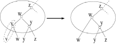
(a) $\mathrm{helper}(v)$ is ancestor of $v$.

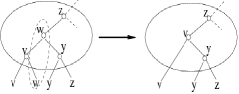
(b) $w$ and $\mathrm{helper}(w)$ share a neighbor.

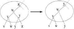
(c) $z$ and $\mathrm{helper}(z)$ do not share neighbors.

(d) $z$ is an heir in Ready state.

Figure 4: Various cases of Leaf deletions

If the adversary removes a leaf node from the system, the healing is accomplished by its neighbors as specified in Algorithm 3.4: FixLeafDeletion. Let $v$ be the deleted leaf node and $p$ be its parent. Let us consider the simple case first. This is when the deleted node had no helper responsibility. This also implies its original parent did not suffer a deletion. Node $p$ simply removes $v$ from the list of its children and then recomputes and redistributes its will.
Now, consider the situation where the deleted node had helper responsibilities. In this case, the one node whose workload has been reduced by this deletion is $p$. Using Algorithm 3.7: MakeLeafWill $v$ hands over the list of its helper responsibilities to $p$. Here, a special case may arise when $v$ is simulating a helper node which has $v$ itself as one of its $\mathrm{hchildren}$. Recall that $\mathrm{parent}(v)$ is $v$’s ancestor closest to $v$ in the tree. This implies that $\mathrm{parent}(v)=\mathrm{hparent}(v)=p$. The only thing that $p$ needs to do if $v$ is deleted is to remove $v$ from its $\mathrm{hchildren}$ and add itself (for consistency). This is the will conveyed by $v$ to $p$. When $v$ is deleted, $p$ simply updates its helper fields. For other cases, $v$ simply sends its helper fields to $p$ to be copied to $p$’s helper reconstruction fields. In this situation, when $v$ is actually deleted the following happens: the helper node that $p$ is simulating is deleted and bypassed by the bypass operation defined earlier. Node $p$ now simulates a new helper node that has the same helper responsibilities previously fulfilled by $v$. In case the deleted leaf node was itself an heir in ready state, $p$ detects this and sets its flags accordingly. Again at the end of the reconstruction, the leaf nodes reconstruct their wills. An example of such a leaf deletion is the deletion of node $d$ at Turn 3 as shown in figure 5.

Important Note: When implementing the pseudocode for Algorithm 3.6: MakeWill, it is important to bear in mind that when $\mathrm{RT}(v)$ is being updated due to a node deletion, most of $\mathrm{SubRT}(v)$ will be unchanged. In fact, only $O(1)$ nodes will need to have their fields updated. These can be found and updated more efficiently by a more detailed algorithm based on case analysis, which we defer to the full version of this paper.

1:  Given a tree $T(V,E)$

2:  Init(T).

3:  while true do

4:     if a vertex $x$ is deleted then

5:        if  $\mathrm{children}(x)$ is EMPTY then

6:           FixLeafDeletion(x)

7:        else

8:           FixNodeDeletion(x)

9:        end if

10:     end if

11:  end while

Algorithm 3.1 Forgiving tree: The main function.

0:  each node of T has a unique ID

1:  for each node $v\in T$ do do

2:     $\mathrm{children}(v)\leftarrow$ children of $v$.

3:     $\mathrm{parent}(v)\leftarrow$ if $v$ is root of T then EMPTY else parent of $v$.

4:     $\mathrm{isreadyheir}(v)\leftarrow false$.

5:     $\mathrm{ishelper}(v)\leftarrow false$.

6:     $\mathrm{hparent}(v)\leftarrow\emph{EMPTY}$.

7:     $\mathrm{hchildren}(v)\leftarrow\emph{EMPTY}$.

8:     $\mathrm{heir}(v)\leftarrow$ if v is a leaf node then EMPTY else child of $v$ with highest ID.

9:     $\mathrm{SubRT}(v)\leftarrow\textsc{generateSubRT}(v)$.

10:     MakeWill($v,\mathrm{SubRT}(v)$).

11:  end for

Algorithm 3.2 Init(T): initialization of the Tree T

Algorithm 3.3 FixNodeDeletion($v$): Self-healing on deletion of internal node

1:  MakeRT($\mathrm{children}(v),\mathrm{parent}(v)$).

2:   let $h=\mathrm{heir}(v)$.Let $p=\mathrm{parent}(v)$

3:  if $\mathrm{isreadyheir}(h)=true$ then

4:     $\mathrm{hparent}(h)$ replaces $v$ by $h$ in $\mathrm{SubRT}(\mathrm{hparent}(h))$.

5:     MakeWill($\mathrm{hparent}(h),\mathrm{SubRT}(\mathrm{hparent}(h))$).

6:  end if

7:  for each node $y\in\mathrm{children}(v)$ do

8:     if $\mathrm{children}(v)$ is EMPTY then

9:        MakeLeafWill($v$).

10:     end if

11:  end for

Algorithm 3.4 FixLeafDeletion($v$): Self-healing on deletion of leaf node

1:  let $p=\mathrm{parent}(v)$

2:  if $\mathrm{ishelper}(p)=false$ then

3:     $p$ removes $v$ from $\mathrm{children}(p)$

4:     $SubRT(p)\leftarrow\textsc{GenerateSubRT}(p)$

5:     MakeWill($p$)

6:  else

7:     Let $z=\mathrm{parent}(v)$.

8:     if $z\neq\mathrm{hparent}(v)$ then

9:        bypass($z$).

10:     end if

11:     $z$ makes edges with $\mathrm{nexthparent}(z)$,$\mathrm{nexthchildren}(z)$.

12:     $\mathrm{hparent}(z)\leftarrow\mathrm{nexthparent}(z)$.

13:     $\mathrm{hchildren}(z)\leftarrow\mathrm{nexthchildren}(z)$.

14:     if $\left|\mathrm{hchildren}(z)\right|$=1 then

15:        $\mathrm{isreadyheir}(z)=true$

16:     end if

17:  end if

18:  for each node $y\in\mathrm{children}(v)$ do

19:     if $\mathrm{children}(v)$ is EMPTY then

20:        MakeLeafWill($v$).

21:     end if

22:  end for

Algorithm 3.5 GenerateSubRT($\mathrm{children}(v)$): Computes the Reconstruction Tree ($\mathrm{RT}$) of $v$ minus a possible helper node simulated by $\mathrm{heir}(v)$.

1:  Let $Lset$ be a set of vertices representing all members of $\mathrm{children}(v)$, and $Iset$ be another set of vertices. representing all members of $\mathrm{children}(v)$ except the one with the highest $ID$.

2:  Arrange $Lset$ in ascending order of their $ID$s.

3:  Using the arranged $Lset$ as leaves and $Iset$ as the internal nodes construct a Balanced Binary Search Tree $\mathrm{SubRT}$ ordered on the nodes $ID$.

4:  return  $\mathrm{SubRT}$

Algorithm 3.6 MakeWill($v,\mathrm{SubRT}(v))$: Makes and distributes the will of v

1:  Let p = $\mathrm{parent}(v)$. Let $rv$ be root of $\mathrm{SubRT}(v)$.

2:  for each node $y\in\mathrm{children}(v)$ do

3:     let $ly$ be the leaf vertex representing $y$ in $\mathrm{SubRT}(v)$. Let $hy$ be the internal node in $\mathrm{SubRT}$ representing $y$.

4:     If $hy$ is $ly$’s parent in $\mathrm{SubRT}(v)$ then $\mathrm{nextparent}(y)\leftarrow$ parent of $hy$ in $\mathrm{SubRT}$ else $\mathrm{nextparent}(y)\leftarrow$ parent of $ly$ in $\mathrm{SubRT}$.

5:     if  $y\neq heir(v)$ then

6:        $\mathrm{nexthchildren}(y)\leftarrow$ children of $hy$ in $\mathrm{SubRT}$.

7:        $\mathrm{nexthparent}(y)\leftarrow$ parent of $hy$ in $\mathrm{SubRT}$.

8:     else

9:        if $\mathrm{ishelper}(v)=true$ then

10:           $\mathrm{nexthchildren}(y)\leftarrow\mathrm{hchildren}(v)$.

11:           $\mathrm{nexthparent}(y)\leftarrow\mathrm{hparent}(v)$.

12:           $\mathrm{nexthparent}(rv)\leftarrow p$.

13:        else

14:           $\mathrm{nexthchildren}(y)\leftarrow rv$.

15:           $\mathrm{nexthparent}(y)\leftarrow p$.

16:           $\mathrm{nexthparent}(rv)\leftarrow y$.

17:        end if

18:     end if

19:  end for

Algorithm 3.7 MakeLeafWill($v$): Leaf node leaves a will for its parent.

1:  let $z=\mathrm{parent}(v)$.

2:  if $z=\mathrm{hparent}(v)$ then

3:     $\mathrm{nexthparent}(z)\leftarrow\mathrm{hparent}(v)$.

4:     $\mathrm{nexthchildren}(z)\leftarrow\mathrm{hchildren}(z)/\{v\}\cup\{z\}$. // $z$ will take on itself as a child of its helper node.

5:  else

6:     $\mathrm{nexthparent}(z)\leftarrow\mathrm{hparent}(v)$.

7:     $\mathrm{nexthchildren}(z)\leftarrow\mathrm{hchildren}(v)$.

8:  end if

Algorithm 3.8 makeRT(children(v),parent(v)): Replace the deleted node by its $\mathrm{RT}$

1:  for each node $x\in$ $\mathrm{children}$(v) do

2:     if $\mathrm{isreadyheir}(x)=true$ then

3:        bypass($x$). // $\mathrm{hparent}(x)$ and $\mathrm{hchildren}(x)$ bypass $x$ and connect themselves.

4:        MakeHelper($x$).

5:     else

6:        $x$ makes edge between itself and $\mathrm{nextparent}(x)$.

7:        $\mathrm{parent}(x)\leftarrow\mathrm{nextparent}(x)$.

8:        MakeHelper($x$).

9:     end if

10:  end for

Algorithm 3.9 MakeHelper($v$): $v$ takes over helper node responsibilities

1:  $v$ makes edges between itself and $\mathrm{nexthchildren}(v)$, and $\mathrm{nexthparent}(v)$.

2:  $\mathrm{hparent}(v)\leftarrow\mathrm{nexthparent}(v)$.

3:  $\mathrm{hchildren}(v)\leftarrow\mathrm{nexthchildren}(v)$.

4:  $\mathrm{ishelper}(v)=true$.

5:  if $|\mathrm{hchildren}(v)|=1$ then

6:     $\mathrm{isreadyheir}(v)=true$. // Only an ’unemployed’ $\mathrm{heir}$ has a single child.

7:  end if

Figure 5: An illustrative sequence of deletions and healings.

4 Results

4.1 Upper Bounds

Let $T$ be the original tree, let $D$ be its diameter, and let $\Delta$ be its maximum degree.

Theorem 1.

The Forgiving Tree has the following properties:

1. The Forgiving Tree increases the degree of any vertex by at most $3$.

2. The Forgiving Tree always has diameter $O(D\log\Delta)$.

3. The latency per deletion and number of messages sent per node per deletion is $O(1)$; each message contains $O(1)$ bits and node IDs.

Proof.

Parts 1 and 3 follow directly by construction of our algorithm. For part 1, we note that for a node $v$, any degree increase for $v$ is imposed by its edges to $\mathrm{hparent}$($v$) and $\mathrm{hchildren}(v)$. By construction, node $v$ can play the role of at most one helper node at any time and the number of $\mathrm{hchildren}$ is never more than $2$, because the reconstruction trees are binary trees. Thus the total degree increase is at most $3$. Part 3 also follows directly by the construction of our algorithm, noting that, because the virtual nodes all have degree at most $3$, healing one deletion results in at most $O(1)$ changes to the edges in each affected reconstruction tree. In fact, the changes to $\mathrm{RT}(w)$ for an affected node $w$ do not require new information, which allows these messages to be computed and distributed in parallel. We leave the details to the full version due to space constraints.

We next show Part 2, that the diameter of the Forgiving Tree is always $O(D\log\Delta)$. We assume that $T$ is rooted with some root $r$ selected arbitrarily and let $p(v)$ be the parent of $v$ in $T$. Fix any node $v_{1}$ in the tree and let $P=v_{1},\ldots,v_{\ell}$ be the path in $T$ from the node $v_{1}$ to the root $v_{\ell}=r$. Let $T^{\prime}$ be the Forgiving Tree data structure after some fixed number of deletions. To simplify notation, if a node $v$ has not been deleted in $T^{\prime}$, we will let root of $\mathrm{RT}(v)$ be $v$ by default. We construct a path $P^{\prime}$ through $T^{\prime}$ from $v_{1}$ to the root of $RT(r)$ as follows. For all $i$ from $1$ to $\ell$, $P^{\prime}$ connects the root of $\mathrm{RT}(v_{i})$ to the root of $\mathrm{RT}(v_{i+j})$ for the smallest $j\geq 1$ such that $\mathrm{RT}(v_{i+j})$ exists. We note that if any nodes remain in $T^{\prime}$, then $\mathrm{RT}(r)$ must still exist and so $P^{\prime}$ connects $v_{1}$ to the root of $\mathrm{RT}(r)$. We further note that the length of $P^{\prime}$ is no more than a factor of $\log\Delta+1$ greater than the length of $P$. To see this, consider the length of the path connecting the root of $\mathrm{RT}(v_{i})$ to the root of $\mathrm{RT}(v_{i+j})$ for the smallest $j\geq 1$ such that $\mathrm{RT}(v_{i+j})$ exists. Such a path can have length at most equal to the log of the number of children of $v_{i+j}$ in $T$, a quantity that can be at most $\log\Delta+1$. The length of the path between the roots will not increase even when nodes in $\mathrm{RT}(v_{i+j})$ are deleted.

Now consider any pair of nodes $x$ and $y$ in $T^{\prime}$. We know from the above that $x$ and $y$ are connected to the root of $\mathrm{RT}(r)$ in $T^{\prime}$ by paths of length at most $h\cdot(\log\Delta+1)$, where $h$ is the height of $T$. We further know that the diameter of $T$, $D$, is at least $h$. It follows directly that the diameter of the Forgiving Tree is never more than $O(D\log\Delta)$. ∎

4.2 Lower Bounds

Theorem 2.

Consider any self-healing algorithm that ensures that: 1) each node increases its degree by at most $\alpha$, for some $\alpha\geq 3$; and 2) the diameter of the graph increases by a multiplicative factor of at most $\beta$. Then for any positive $\Delta$, for some initial graph with maximum degree $\Delta$, it must be the case that $\alpha^{2\beta+1}\geq\Delta$.

Proof.

Let $G$ be a star on $\Delta+1$ vertices, where $x$ is the root node, and $x$ has $\Delta$ edges with each of the other nodes in the graph. Let $G^{\prime}$ be the graph created after the adversary deletes the node $x$. Consider a breadth first search tree, $T$, rooted at some arbitrary node $y$ in $G^{\prime}$. We know that the self-healing algorithm can increase the degree of each node by at most $\alpha$, thus every node in $T$ can have at most $\alpha+1$ children. Let $h$ be the height of $T$. Then we know that $1+(\alpha+1)\sum_{i=0}^{h-1}\alpha^{i}\geq\Delta$. This implies that $\alpha^{h+1}\geq\Delta$ for $\alpha\geq 3$, or ${h+1}\geq\log_{\alpha}\Delta$. Since the diameter of $G$ is $2$, we know that $\beta=h/2$, and thus $2\beta+1\geq\log_{\alpha}\Delta$. Raising $\alpha$ to the power of both sides, we get that $\alpha^{2\beta+1}\geq\Delta$. ∎

We note that this lower-bound compares favorable with the general result achieved with our data structure. The Forgiving Tree can be modified so that it ensures that 1) the degree of any node increases by no more than $\alpha$ for any $\alpha\geq 3$; and that the diameter increases by no more than a multiplicative factor of $\beta\leq 2\log_{\alpha}\Delta+2$. Thus we can ensure that $\alpha^{(1/2)(\beta-1)}\leq\Delta$.

5 Conclusion

We have presented a distributed data structure that withstands repeated adversarial node deletions by adding a small number of new edges after each deletion. Our data structure ensures two key properties, even when up to all nodes in the network have been deleted. First, the diameter of the network never increases by more than $O(\log\Delta)$ times its original diameter, where $\Delta$ is the maximum original degree of any node. For many peer-to-peer systems, $\Delta$ is at most polylogarithmic, and so the diameter would increase by no more than a $O(\log\log n)$ multiplicative factor. Second, no node ever increases its degree by more than $3$ over its original degree.

Several open problems remain including the following. Can we protect other invariants? For example, can we design a distributed data structure to ensure that the stretch between any pair of nodes increases by no more than a certain amount? Can we design algorithms for less flexible networks such as sensor networks? For example, what if the only edges we can add are those that span a small distance in the original network? Finally, can we extend the concept of self-healing to other objects besides graphs? For example, can we design algorithms to rewire a circuit so that it maintains its functionality even when multiple gates fail?

References

- [1] D. Andersen, H. Balakrishnan, F. Kaashoek, and R. Morris. Resilient overlay networks. SIGOPS Oper. Syst. Rev., 35(5):131–145, 2001.
- [2] V. Arak. What happened on August 16, August 2007. http://heartbeat.skype.com/2007/08/what-happened-on-august-16.html.
- [3] I. Boman, J. Saia, C. T. Abdallah, and E. Schamiloglu. Brief announcement: Self-healing algorithms for reconfigurable networks. In Symposium on Stabilization, Safety, and Security of Distributed Systems(SSS), 2006.
- [4] E. Cohen. Size-estimation framework with applications to transitive closure and reachability. In Proceedings of the Foundations of Computer Science (FOCS), 1994.
- [5] R. D. Doverspike and B. Wilson. Comparison of capacity efficiency of dcs network restoration routing techniques. J. Network Syst. Manage., 2(2), 1994.
- [6] K. Fisher. Skype talks of ”perfect storm” that caused outage, clarifies blame, August 2007. http://arstechnica.com/news.ars/post/20070821-skype-talks-of-perfect-storm.html.
- [7] T. Frisanco. Optimal spare capacity design for various protection switchingmethods in atm networks. In Communications, 1997. ICC 97 Montreal, ’Towards the Knowledge Millennium’. 1997 IEEE International Conference on, volume 1, pages 293–298, 1997.
- [8] S. Goel, S. Belardo, and L. Iwan. A resilient network that can operate under duress: To support communication between government agencies during crisis situations. Proceedings of the 37th Hawaii International Conference on System Sciences, 0-7695-2056-1/04:1–11, 2004.
- [9] Y. Hayashi and T. Miyazaki. Emergent rewirings for cascades on correlated networks. cond-mat/0503615, 2005.
- [10] P. Holme and B. J. Kim. Vertex overload breakdown in evolving networks. Physical Review E, 65:066109, 2002.
- [11] R. R. Iraschko, M. H. MacGregor, and W. D. Grover. Optimal capacity placement for path restoration in stm or atm mesh-survivable networks. IEEE/ACM Trans. Netw., 6(3):325–336, 1998.
- [12] O. Malik. Does Skype Outage Expose P2P s Limitations?, August 2007. http://gigaom.com/2007/08/16/skype-outage.
- [13] M. Medard, S. G. Finn, and R. A. Barry. Redundant trees for preplanned recovery in arbitrary vertex-redundant or edge-redundant graphs. IEEE/ACM Transactions on Networking, 7(5):641–652, 1999.
- [14] M. Moore. Skype’s outage not a hang-up for user base, August 2007. http://www.usatoday.com/tech/wireless/phones/2007-08-24-skype-outage-effects-N.htm.
- [15] A. E. Motter. Cascade control and defense in complex networks. Physical Review Letters, 93:098701, 2004.
- [16] A. E. Motter and Y.-C. Lai. Cascade-based attacks on complex networks. Physical Review E, 66:065102, 2002.
- [17] K. Murakami and H. S. Kim. Comparative study on restoration schemes of survivable ATM networks. In INFOCOM (1), pages 345–352, 1997.
- [18] B. Ray. Skype hangs up on users, August 2007. http://www.theregister.co.uk/2007/08/16/skype_down/.
- [19] J. Saia and A. Trehan. Picking up the pieces: Self-healing in reconfigurable networks. In IEEE International Parallel & Distributed Processing Symposium, 2008.
- [20] B. Stone. Skype: Microsoft Update Took Us Down, August 2007. http://bits.blogs.nytimes.com/2007/08/20/skype-microsoft-update-took-us-down.
- [21] B. van Caenegem, N. Wauters, and P. Demeester. Spare capacity assignment for different restoration strategies in mesh survivable networks. In Communications, 1997. ICC 97 Montreal, ’Towards the Knowledge Millennium’. 1997 IEEE International Conference on, volume 1, pages 288–292, 1997.
- [22] Y. Xiong and L. G. Mason. Restoration strategies and spare capacity requirements in self-healing atm networks. IEEE/ACM Trans. Netw., 7(1):98–110, 1999.