Three-dimensional stability of magnetically confined mountains on accreting neutron stars

Abstract

We examine the hydromagnetic stability of magnetically confined mountains, which arise when material accumulates at the magnetic poles of an accreting neutron star. We extend a previous axisymmetric stability analysis by performing three-dimensional simulations using the ideal-magnetohydrodynamic (ideal-MHD) code zeus-mp, investigating the role played by boundary conditions, accreted mass, stellar curvature, and (briefly) toroidal magnetic field strength. We find that axisymmetric equilibria are susceptible to the undular sub-mode of the Parker instability but are not disrupted. The line-tying boundary condition at the stellar surface is crucial in stabilizing the mountain. The nonlinear three-dimensional saturation state of the instability is characterized by a small degree of nonaxisymmetry ($\la 0.1$ per cent) and a mass ellipticity of $\epsilon\sim 10^{-5}$ for an accreted mass of $M_{a}=10^{-5}M_{\odot}$. Hence there is a good prospect of detecting gravitational waves from accreting millisecond pulsars with long-baseline interferometers such as Advanced LIGO. We also investigate the ideal-MHD spectrum of the system, finding that long-wavelength poloidal modes are suppressed in favour of toroidal modes in the nonaxisymmetric saturation state.

1 Introduction

There exists strong observational evidence that the magnetic dipole moment of accreting neutron stars in X-ray binaries, $\mu$, decreases with accreted mass, $M_{a}$ (Taam & van de Heuvel, 1986; van den Heuvel & Bitzaraki, 1995), although Wijers (1997) noted that extra variables may enter this relation. Numerous mechanisms for field reduction have been proposed, such as accelerated Ohmic decay (Konar & Bhattacharya, 1997; Urpin & Konenkov, 1997), vortex-fluxoid interactions in the superconducting core (Muslimov & Tsygan, 1985; Srinivasan et al., 1990), and magnetic screening or burial (Bisnovatyi-Kogan & Komberg, 1974; Romani, 1990; Zhang, 1998; Payne & Melatos, 2004; Lovelace et al., 2005). The reader is referred to Melatos & Phinney (2001) for a comparative review.

Magnetic burial occurs when accreted plasma flowing inside the Alfvén radius is chanelled onto the magnetic poles of the neutron star. The hydrostatic pressure at the base of the accreted column overcomes the magnetic tension of the magnetic field lines and spreads equatorwards, thereby distorting the frozen-in magnetic flux (Melatos & Phinney, 2001). Payne & Melatos (2004), hereafter PM04, computed self-consistently the unique quasistatic sequence of ideal-MHD equilibria that describes how burial proceeds as a function of $M_{a}$, while respecting the flux freezing constraint of ideal MHD. They found that the magnetic field is compressed into an equatorial belt, which confines the accreted mountain at the poles. A key result is that $\mu$ is reduced significantly once $M_{a}$ exceeds $\sim 10^{-5}M_{\odot}$, five orders of magnitude above previous estimates (Brown & Bildsten, 1998; Litwin et al., 2001).

Generally speaking, one expects highly distorted hydromagnetic equilibria like those in PM04 to be disrupted on the Alfvén time-scale by a plethora of MHD instabilities. Surprisingly, however, Payne & Melatos (2007) (hereafter PM07) found the equilibria to be stable to axisymmetric ideal-MHD modes. When kicked, the mountain performs radial and lateral oscillations corresponding to global Alfvén and compressional modes, but it remains intact.

An axisymmetric analysis, however, excludes instabilities involving toroidal modes and is therefore incomplete. In general, three-dimensional effects alter MHD stability, quantitatively and qualitatively. For example, Matsumoto & Shibata (1992) found the growth rate of the three-dimensional Parker instability to be higher than that of its two-dimensional counterpart. Masada et al. (2006) proved that newly born neutron stars containing a toroidal field are stable to the axisymmetric magneto-rotational instability yet unstable to its nonaxisymmetric counterpart. Differences between the two- and three-dimensional stability of MHD equilibria are also observed in a variety of solar contexts (Priest, 1984) and in tokamaks (Lifschitz, 1989; Goedbloed & Poedts, 2004).

The central aim of this paper is to perform fully three-dimensional, ideal-MHD simulations to assess the stability of magnetic mountains, generalizing PM07. Importantly, we compute not just the linear growth rate but also the nonlinear saturation state of any unstable modes. The latter property is what matters over the long accretion time-scale when evaluating magnetic burial as the cause of the observed reduction in $\mu$ (Payne, 2005), the persistence of millisecond oscillations in type-I X-ray bursts (Payne & Melatos, 2006b), and gravitational radiation from magnetic mountains (Melatos & Payne, 2005; Payne & Melatos, 2006a).

The structure of the paper is as follows. We introduce our numerical setup in section 2 and validate it against previous axisymmetric results in section 3, characterizing the controlling influence of the boundary conditions for the first time. In section 4, we present three-dimensional simulations, which display growth of unstable toroidal modes. The instability is classified according to its dispersive properties and energetics, and the nonlinear saturation state is computed as a function of $M_{a}$. We compute the spectrum of global MHD oscillations in section 5. Resistive effects are postponed to a future paper.

2 Numerical model

The accretion problem contains two fundamentally different time-scales: the long accretion time ($\sim 10^{8}$ yr) and the short Alfven time ($\sim 10^{-3}$ s). The wide discrepancy prevents us from treating the accretion problem dynamically, i.e. in a full MHD simulation, where mass is added through the outer boundary onto an initially dipolar field. Instead, for a given value of $M_{a}$, we compute the magnetohydrostatic equilibria, using the Grad-Shafranov solver developed by PM04, then load it into the ideal-MHD solver zeus-mp (Hayes et al., 2006) to test its hydromagnetic stability on the Alfvén time-scale $\tau_{\mathrm{A}}$. We find below that all quantities reach their saturation values after $\sim 10\tau_{A}\sim 10^{-2}$ s at a particular value of $M_{a}$ (e.g. $10^{-4}M_{\odot}$). As $M_{a}$ changes slowly, over $\sim 10^{8}$ yr, the saturation values adjust in a quasistatic way on the Alfvén time-scale. In practice, to study a different value of $M_{a}$ numerically, we recalculate the Grad-Shafranov eqilibrium and load the new equilibrium into zeus-mp.

2.1 Magnetic mountain equilibria

Analytic and numerical recipes for calculating self-consistent ideal-MHD equilibria for magnetic mountains are set out in PM04. Here, we briefly restate the main points for the convenience of the reader.

An axisymmetric equilibrium is generated by a scalar flux function $\psi(r,\theta)$, such that the magnetic field

$$\mathbf{B}=\frac{\nabla\psi}{r\sin\theta}\times\hat{\mathbf{e}}_{\phi}$$ (1)

automatically satisfies $\nabla\mathbf{\mn@boldsymbol{\cdot}}\mathbf{B}=0$. We employ the usual spherical coordinates $(r,\theta,\phi)$, where $\theta=0$ corresponds to the symmetry axis of the magnetic field before accretion. In the static limit, the mass conservation and MHD induction equations are identically satisfied, while the component of the momentum equation transverse to $\mathbf{B}$ reduces to a second order, nonlinear, elliptic partial differential equation for $\psi$, the Grad-Shafranov (GS) equation (PM04):

$$\Delta^{2}\psi=-F^{\prime}(\psi)\exp[-(\varphi-\varphi_{0})/c_{s}^{2}],$$ (2)

with

$$\Delta^{2}=\frac{1}{\mu_{0}r^{2}\sin^{2}\theta}\left[\frac{\partial^{2}}{\partial r^{2}}+\frac{\sin\theta}{r^{2}}\frac{\partial}{\partial\theta}\left(\frac{1}{\sin\theta}\frac{\partial}{\partial\theta}\right)\right].$$ (3)

Formally, $F(\psi)$ is an arbitrary function. However, the ideal-MHD flux-freezing constraint, that matter cannot cross flux surfaces, imposes an additional conservation law on the mass-flux ratio $\mathrm{d}M/\mathrm{d}\psi$,

$$F(\psi)=\frac{c_{s}^{2}}{2\pi}\frac{\mathrm{d}M}{\mathrm{d}\psi}\left\{\int\mathrm{d}s\,r\sin\theta|\nabla\psi|^{-1}\mathrm{e}^{-(\varphi-\varphi_{0})/c_{s}^{2}}\right\}^{-1},$$ (4)

which determines $F(\psi)$ uniquely when solved simultaneously with (2). The integration in (4) is performed along the field line $\psi=\mathrm{const}$, $\phi=\mathrm{const}$. The solution is insensitive to the exact form of $\mathrm{d}M/\mathrm{d}\psi$; we thus distribute the accreted mass $M_{a}$ uniformly over $0\leq\psi\leq\psi_{a}$, where $\psi_{a}$ is the flux enclosed within the polar cap, and take $\psi$ to be dipolar, initially, with hemispheric flux $\psi_{\ast}$.

In writing (2) and (5), we approximate the gravitational field as uniform over the height of the mountain, and hence write the gravitational potential $\varphi$ as

$$\varphi=GM_{\ast}r/R_{\ast}^{2},$$ (5)

with $\varphi_{0}=GM_{\ast}/R_{\ast}$, where $M_{\ast}$ and $R_{\ast}$ denote the stellar mass and radius respectively. We also assume an isothermal equation of state, $\rho=c_{s}^{2}p$, where $c_{s}$ denotes the sound speed.

By working in the ideal-MHD limit, we neglect elastic stresses (Melatos & Phinney, 2001; Haskell et al., 2006; Owen, 2006), the Hall drift (Geppert & Rheinhardt, 2002; Cumming et al., 2004; Pons & Geppert, 2007), and Ohmic diffusion (Romani, 1990; Geppert & Urpin, 1994). In particular, Ohmic diffusion causes the mass quadrupole moment of the magnetic mountain (and $\mu$) to saturate above a certain value of $M_{a}$ and may also affect the stability to resistive MHD (e.g. ballooning) modes. We defer investigating these resistive effects to a forthcoming paper [Vigelius & Melatos (in preparation)].

We solve (2) and (4) simultaneously using the relaxation algorithm described in PM04, subject to the boundary conditions $\psi(R_{\ast},\theta)=\psi_{\ast}\sin^{2}\theta$ (line tying at the surface), $\partial\psi/\partial r(R_{m},\theta)=0$ at the outer boundary $r=R_{m}$, $\psi(r,0)=0$, and $\partial\psi/\partial\theta(r,\pi/2)=0$ (north-south symmetry).

2.2 Evolution in ZEUS-MP

In this paper, we explore numerically how the axisymmetric GS equilibria evolve when subjected to a variety of initial and boundary conditions in three dimensions. To achieve this, we employ the parallelized, general purpose, time-dependent, ideal-MHD solver zeus-mp (Hayes et al., 2006). zeus-mp integrates the equations of ideal MHD, discretized on a fixed staggered grid. The hydrodynamic part is based on a finite-difference advection scheme accurate to second order in time and space. The magnetic tension force and the induction equation are solved via the method of characteristics and constrained transport (MOCCT) (Hawley & Stone, 1995), whose numerical implementation in zeus-mp is described in detail by Hayes et al. (2006).

We initialize zeus-mp with an equilibrium computed by the GS code and described by $\mathbf{B}(r,\theta)$ and $\rho(r,\theta)$, rotated about the $z$ axis to generate cylindrical symmetry. We introduce initial perturbations by taking advantage of the numerical noise produced by the transition between grids in the GS code and zeus-mp.

We adopt dimensionless variables in zeus-mp satisfying $\mu_{0}=G=c_{s}=h_{0}=1$, where $h_{0}=c_{s}^{2}R_{\ast}^{2}/GM_{\ast}$ denotes the hydrostatic scale height. The basic units of mass, magnetic field, and time are then $M_{0}=h_{0}c_{s}^{2}/G$, $B_{0}=[c_{s}^{4}/(Gh_{0}^{2})]^{1/2}$, and $\tau_{0}=h_{0}/c_{s}$. The grid and boundary conditions are specified in appendix A.

2.3 Curvature rescaling

In general, the characteristic length-scale for radial gradients ($h_{0}$) is much smaller than the length-scale for latitudinal gradients $R_{\ast}$, creating numerical difficulties. However, in the small-$M_{a}$ limit, it can be shown analytically (PM04, PM07) that the structure of the magnetic mountain depends on $R_{\ast}$ and $M_{\ast}$ through the combination $h_{0}\propto R_{\ast}^{2}/M_{\ast}$, not separately. We therefore artificially reduce $R_{\ast}$ and $M_{\ast}$, while keeping $h_{0}$ fixed, to render the problem tractable computationally. It is important to bear in mind that invariance of the equilibrium structure under this curvature rescaling does not imply invariance of the dynamical behaviour, nor is it necessarily applicable at large $M_{a}$.

A standard neutron star has $M_{\ast}=1.4M_{\odot}$, $R_{\ast}=10^{6}$ cm, $B_{\ast}=10^{12}$ G, and $c_{s}=10^{8}$ cm s^-1, giving $h_{0}=53.82$ cm, $a=R_{\ast}/h_{0}=1.9\times 10^{4}$, and $\tau_{0}=5.4\times 10^{-7}$ s. We rescale the star to $M_{\ast}^{\prime}=1.0\times 10^{-5}M_{\odot}$ and $R_{\ast}^{\prime}=2.7\times 10^{3}$ cm, reducing $a$ to 50 while keeping it large. The base units for this rescaled star (see section 2.2) are then $M_{0}=8.1\times 10^{24}$ g, $\rho_{0}=5.2\times 10^{19}$ g cm^-3, $B_{0}=7.2\times 10^{17}$ G, and $\tau_{0}=5.4\times 10^{-7}$ s. The critical accreted mass above which the star’s magnetic moment starts to change, $M_{c}$, is defined by equation (30) of PM04:

$$\frac{M_{c}}{M_{\odot}}=6.2\times 10^{-15}\left(\frac{a}{50}\right)^{4}\left(\frac{B_{\ast}}{10^{12}\mathrm{G}}\right)^{2}\left(\frac{c_{s}}{10^{8}\mathrm{cm\;s}^{-1}}\right)^{-4}.$$ (6)

A characteristic time-scale for the MHD response of the mountain is the Alfvén pole-equator crossing time, $\tau_{\mathrm{A}}=\pi R_{\ast}/(2v_{\mathrm{A}})$, where $v_{\mathrm{A}}=(B^{2}/\mu_{0}\rho)^{1/2}$ is the Alfvén speed. Clearly, $v_{\mathrm{A}}$ is a function of position and time, so the definition of $\tau_{\mathrm{A}}$ is somewhat arbitrary. Typically, at the equator, we find $B\sim 10^{-6}B_{0}$ and $\rho\sim 10^{-11}\rho_{0}$, empirically implying $\tau_{\mathrm{A}}\approx 250\tau_{0}$.

3 Axisymmetric stability and global oscillations

Table 1: Simulation parameters. $M_{a}$ is the accreted mass, in units of the characteristic mass $M_{c}$ (section 2.3), and $a=R_{\ast}/h_{0}$ measures the curvature of the rescaled star (section 2.3). The conditions at the outer boundary ($r=R_{m}$) are either outflow (zero gradient in all field variables) or inflow (pinned magnetic field); cf. also appendix A.

Model	$M_{a}/M_{c}$	$a$	Axisymmetry	Boundary
A	1.0	50	yes	outflow
B	1.0	50	yes	inflow
D	1.0	50	no	outflow
E	1.0	50	no	inflow
F	0.6	50	no	outflow
G	1.4	50	no	outflow
J	1.0	75	no	outflow
K	1.0	100	no	outflow

PM07 demonstrated the axisymmetric stability of magnetic mountains using the serial ideal-MHD solver zeus-3d. Here, we start by repeating these axisymmetric simulations in the parallel solver zeus-mp, in order to verify the mountain implementation in zeus-3d and zeus-mp, generate an axisymmetric reference model, and understand the effect of the boundary conditions, which were not investigated fully in previous work. The simulation parameters are detailed in Table 1 (models A and B).

Figure 1: Meridional section of model A at $t/\tau_{\mathrm{A}}=0,0.4,1,1.8,2.4,3.6$ (top left to bottom right). Shown are density contours (dashed curves) with values $\log_{10}(\rho/\rho_{0}^{\prime})=-13,-12,-11,-10.7,-10.5,-10.3$, and flux surfaces with footpoints at $r=R_{\ast}$, $\theta=0.10,0.12,0.15,0.20,0.39,0.79$ (solid curves). Lateral oscillations of the equatorial field lines are clearly visible. The outflow boundary condition at $r=R_{m}$ makes the field lines flare towards the magnetic pole. This is visible most clearly for the line whose footpoint lies at $\theta=0.39$.

3.1 Reference model

Model A, in which we set $M_{a}/M_{c}=1.0$ and the outer boundary condition to outflow, serves as a reference case. Fig. 1 displays a time series of six $r$-$\theta$ sections for $0\leq t/\tau_{A}\leq 3.6$, showing density contours (dashed curves) and the magnetic field lines projected into the plane $\phi=0$ (solid curves). The axisymmetric equilibrium (top-left panel) reveals how the bulk matter is contained at the magnetic pole by the tension of the distorted magnetic field.

The mountain in Fig. 1 performs damped lateral oscillations without being disrupted. The (unexpected) stability of this configuration is due to two factors. First, the configuration is already the final, saturated state of the nonlinear Parker instability, which is reached quasistatically during slow accretion (PM04; Mouschovias, 1974). Second, line-tying of the magnetic field at $r=R_{\ast}$ significantly changes the structure of the MHD wave spectrum in a way that enhances stability. Goedbloed & Halberstadt (1994) found that, in a homogenous plasma, a superposition of Alfvén- and magnetosonic waves is needed to satisfy the line-tying boundary conditions. As a consequence, the basic, unmixed MHD modes are not eigenfunctions of the linear force operator, and thus the spectrum is modified.

The mass quadrupole moments,

$$Q_{ij}=\int d^{3}x^{\prime}\,(3x_{i}^{\prime}x_{j}^{\prime}-r^{\prime 2}\delta_{ij})\rho(\mathbf{x^{\prime}}),$$ (7)

of the mountain in Fig. 1 are plotted versus time in Fig. 2. We note first that $Q_{12}=0$ and $Q_{22}=-Q_{33}/2$, as expected for an axisymmetric system. We can compare Fig. 2 directly with the ellipticity $\epsilon\propto Q_{33}$ computed by Payne & Melatos (2006a).. These authors found two dominant global modes, an Alfvén and an acoustic mode, claimed to be analogous to the fundamental modes of a gravitating, magnetized plasma slab. We cannot resolve the compressional modes in Fig. 2, but the latitudinal (Alfvén) mode is clearly visible through the oscillations in $Q_{22}$ and $Q_{33}$.

Figure 2: Mass quadrupole moments for model A, normalised to the maximum of $Q_{33}$ ($1.3\times 10^{25}$ g cm²), as a function of time in units Alfvén time. We find $Q_{22}=-Q_{33}/2$ and $Q_{12}=0$, as expected for an axisymmetric configuration. The global Alfvén oscillation is damped by numerical viscosity.

An oscillation cycle proceeds as follows. The first minimum of $Q_{33}$, and hence $\epsilon$, at $t=0.4\tau_{\mathrm{A}}$ in Fig. 2, corresponds to the top right panel of Fig. 1. The mountain withdraws radially and poleward. Polar field lines move closer to the magnetic pole, while equatorial field lines are drawn towards the equator. At $\tau=\tau_{\mathrm{A}}$, the mountain spreads and $Q_{33}$ reaches a maximum in Fig. 2. The damping observed in Fig. 2 arises solely from numerical dissipation; neither viscosity nor resistivity are included in our version of zeus-mp.

3.2 Outer boundary

The “flaring up” of magnetic field lines at the pole, observed by PM07, is an artifact of the outflow boundary condition at $r=R_{m}$. In order to check this, we repeat the simulation of model A but switch to an inflow boundary condition (model B). The density distribution is similar in the two models, as is clear from Fig. 3. However, the inflow BC artifically pins the magnetic field to the outer boundary, introducing magnetic field discrepancies (mostly in the outer layers, where $\rho$ is negligible).

Figure 3: Meridional section of model B, showing density (left) and projected magnetic field (right) at $t/\tau_{\mathrm{A}}=3.6$ (solid curves). The field lines are pinned to the outer $r$ boundary by the inflow boundary condition. For comparison, the density and magnetic field of model A are overplotted (dotted curves).

Alfvén waves are similar to transverse waves on a string, where the magnetic tension provides the restoring force. Models A and B are therefore equivalent to a vibrating string with one end free and fixed respectively. We expect the oscillation frequency of the fundamental mode in model B to be twice that of model A. This is indeed observed in the oscillations of the quadrupole moments, displayed in Fig. 4: $Q_{22}$ and $Q_{33}$ in Fig. 4 oscillate at $0.6$ times the period in Fig. 2. A comprehensive analytic computation of the MHD spectrum, including discrete and continuous components, will be attempted in a forthcoming paper.

Figure 4: Mass quadrupole moments for model B, normalised to the maximum of $Q_{33}$ ($1.3\times 10^{25}$ g cm²) as a function of time in units of the Alfvén time. We find $Q_{22}=-Q_{33}/2$ and $Q_{12}=0$, as expected for an axisymmetric configuration. The mountain performs damped lateral oscillations with twice the frequency of model A.

3.3 Uniform toroidal field

There are strong theoretical indications that the magnetorotational instability (Balbus & Hawley, 1998) acts during core collapse supernova explosions to generate a substantial toroidal field component $B_{\phi}\sim B_{p}$ beneath the stellar surface (Cutler, 2002; Akiyama et al., 2003). The hydromagnetic stability of equilibria with $B_{\phi}\neq 0$ will be discussed thoroughly in a forthcoming paper. In this subsection, for completeness, we present the results of a preliminary investigation.

Let us rerun model A with the same initial conditions while applying a uniform $B_{\phi}=10^{-7}B_{0}=0.35B_{p}$ throughout the integration volume and at $r=R_{\ast}$, where the poloidal field component is defined as $B_{p}=(B_{r}^{2}+B_{\theta}^{2})^{1/2}$, taken at the point $[\tilde{x}=(r-R_{\ast})/h_{0},\theta,\phi]=(10^{-3},0.012,0)$. $B_{\phi}$ is uniform only initially and is allowed to evolve nonuniformly as zeus-mp proceeds. This procedure leads to a non-equilibrium configuration, because we do not generalise and solve again the GS equation (2) to accomodate $B_{\phi}\neq 0$. Nevertheless, it provides us with some insight into the stability of a field with nonzero pitch angle.

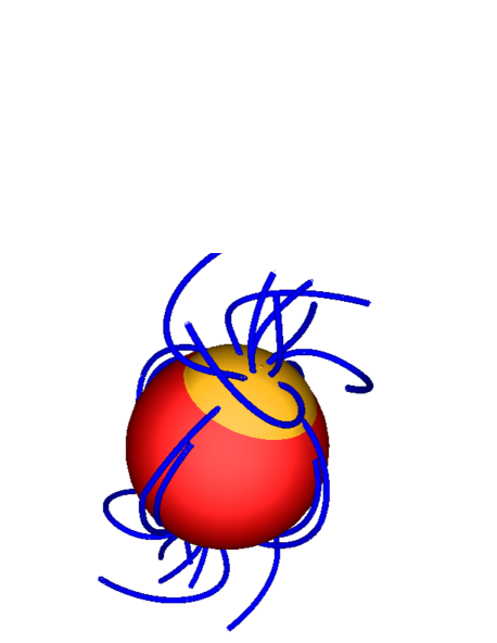
Figure 5: Model A repeated with the same parameters as in Table 1 including a uniform toroidal field $B_{\phi}=10^{-7}B_{0}=0.35B_{p}$. The mountain is defined by the orange isosurface $\rho(r,\theta,\phi)=1.04\times 10^{9}$ g cm³, while red denotes the neutron star surface $r=R_{\ast}$. In order to improve visibility, all length scales of the mountain and the field lines (blue) are magnified five-fold. The field exhibits a helical topology, which is most distinct in the polar flux tubes where the poloidal contribution is weakest.

Figure 6: Mass ellipticity of model A with (solid) and without (dotted) a uniform $B_{\phi}$. The toroidal field component leads to a shorter oscillation period and to a higher saturation ellipticity.

Fig. 5 displays the result of this numerical experiment after $t=7.4\tau_{A}$. The toroidal field component creates a helical field topology in the polar region far from the surface, where the poloidal field is comparably weak. In the equatorial region, however, the poloidal field is still dominant and the structure remains unchanged from Fig. 1. Remarkably, the toroidal field does not alter the stability of the system qualitatively, at least for the parameters of model A [We expect a stronger effect in other parameter regimes; see Lifschitz (1989); Goedbloed & Poedts (2004)]. The ellipticity, displayed in Fig. 6 (solid curve), exhibits characteristic oscillations with a period $\sim 30$ per cent smaller than that of the purely poloidal configuration (dotted curve), which can be explained simply by the increase in the Alfven speed. In addition, the saturation ellipticity is $\sim 3$ per cent higher than in model A; the magnetic tension increases with $B$, sustaining the mountain at a lower colatitude.

4 Nonaxisymmetric stability

We turn now to the three-dimensional evolution of a magnetised mountain in zeus-mp. The chief finding, presented below, is that the initial (axisymmetric) configuration becomes unstable to toroidal perturbations, but that, after a brief transition phase, the system settles into a new (nearly axisymmetric) state, which is stable in the long term. Section 4.1 compares the results to the axisymmetric reference model A. The magnetic and mass multipole moments are computed in section 4.2, the influence of the boundary conditions is considered in section 4.3, and the component-wise evolution of the energy is examined in section 4.4. A scaling of the mass quadrupole moment versus $M_{a}$ is derived empirically in section 4.5. The curvature rescaling is verified in section 4.6.

4.1 General features

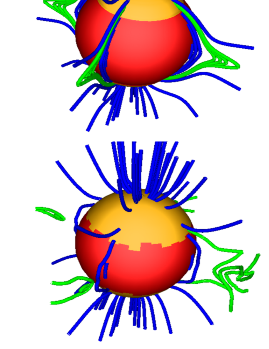
Figure 7: Density and magnetic field of model D at $\tau/\tau_{\mathrm{A}}=0,1,2,3,4,5$ (from top left to bottom right). The mountain is defined by the orange isosurface $\rho(r,\theta,\phi)=1.04\times 10^{9}$ g cm³, while red indicates the neutron star surface $r=R_{\ast}$. In order to improve visibility, all length scales of the mountain and the field lines are magnified five-fold. The mountain becomes unstable to toroidal modes at $\tau\approx 0.8\tau_{\mathrm{A}}$. It subsequently relaxes to a new nonaxisymmetric equilibrium. The footpoint of the blue fieldlines is at the stellar surface while green fieldlines are traced starting from the equator. Green field lines eventually become topologically disconnected (see text).

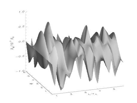
Figure 8: Evolution of the azimuthal magnetic field component $B_{\phi}$ at $(\tilde{x},\theta)=(10^{-3},0.01)$ in model D as a function of longitude $\phi$ (in radians) and time $t$ (in units of the Alfvén time.)

Model D starts from the same configuration as model A ($M_{a}/M_{c}=1.0$, outflow at $r=R_{m}$) but is evolved in three dimensions. Six snapshots of a density isosurface (orange) and magnetic field lines (blue) are depicted in Fig. 7. At $\tau\approx 0.8\tau_{\mathrm{A}}=200\tau_{0}$, the system undergoes a violent transition. The field lines bend in the $\phi$ direction, indicating that the initial axisymmetric configuration is unstable to toroidal modes, a channel that is evidently not present in axisymmetric simulations. This hypothesis is supported by Fig. 8 which plots $B_{\phi}$ at $\tilde{x}=10^{-3}$ and $\theta=0.01$ as a function of $\phi$ and $t$. The magnetic field takes the form of an azimuthal travelling wave $B_{\phi}\sim\exp[\mathrm{i}(m\phi-\omega t)]$. From Fig. 8, we measure the phase speed to be approximately $v_{\mathrm{p}}=\omega R_{\ast}/m=27v_{\mathrm{A}}$, where the Alfvén speed $v_{\mathrm{A}}$ is measured at $(\tilde{x},\theta,\phi)=(10^{-3},0.01,0.1)$ and we assume $m=1$. An inhomogenous plasma generally supports mixed magnetosonic/Alfvén modes, so $v_{\phi}$ does not necessarily equal $v_{\mathrm{A}}$ or the fast/slow magnetosonic speed. The magnitude of $B_{\phi}$ is comparable to the magnitude of the polar magnetic field $B_{\mathrm{p}}=2.9\times 10^{-7}B_{0}$.

The deviations of the mountain isosurface, defined by $\rho(r,\theta,\phi)=1.04\times 10^{9}$ g cm³, from axisymmetry are small ($\la 5$ per cent laterally and $\la 0.06$ per cent radially during the transition phase). The isosurface spreads outward by $\sim 32$ per cent relative to ites initial position.

Figure 9: $|B_{\phi}|$ at $(\tilde{x},\theta,\phi)=(10^{-3},1.5,1.3)$ for model D, simulated at higher resolution ($N_{\phi}=32$, solid) and lower resolution ($N_{\phi}=8$, dashed). Small wavelength perturbations grow faster. We track the absolute value of $|B_{\phi}|$ in order to isolate better the dominant mode, as the system exists in a superposition of stable and unstable modes, and $B_{\phi}$ switches sign.

Fig. 9 demonstrates how the instability grows. We plot $|B_{\phi}|$ at the (arbitrary) position $(r,\theta,\phi)=(R_{\ast},1.5,1.3)$ versus time. The solid curve corresponds to a higher toroidal resolution ($N_{\phi}=32$ grid cells in $\phi$ direction) than the dashed curve ($N_{\phi}=8$). We note first that $|B_{\phi}|$ grows exponentially with time, as expected in the linear regime. The growth rate is measured to be $\Gamma=\mathrm{Im}(\omega)=0.05\tau_{0}^{-1}=12.5\tau_{\mathrm{A}}^{-1}$. Second, the instability is manifestly associated with toroidal modes. The magnetic perturbation, $\delta\mathbf{B}$, induced by a linear Lagrangian displacement $\mn@boldsymbol{\xi}$ is $\delta\mathbf{B}=\nabla\times(\mn@boldsymbol{\xi}\times\mathbf{B})$. By writing out the vector components, one sees that $\delta B_{\phi}\neq 0$ implies $\xi_{\phi}\neq 0$, provided the unperturbed field has the form $\mathbf{B}=B_{r}(r,\theta)\hat{\mathbf{e}}_{r}+B_{\theta}(r,\theta)\hat{\mathbf{e}}_{\theta}$.

The dashed curve in Fig. 9 tracks $|B_{\phi}|$ for a simulation carried out at a lower resolution ($N_{\phi}=8$). The instability grows significantly slower with $\Gamma=\mathrm{Im}(\omega)=0.02\tau_{0}^{-1}=5\tau_{\mathrm{A}}^{-1}$. We conclude that $\Gamma$ scales with the wavelength $\lambda$ of the perturbation roughly as $\lambda^{-1/2}$. The piecewise-straight appearance of the dashed curve in Fig. 9 shows that the global oscillations are governed by a superposition of unstable (growing) and stable wave modes.

What type of instability is at work here? In order to answer that question, we first write down the change in potential energy associated with a Lagrangian displacement $\mn@boldsymbol{\xi}$ in a form that reveals the physical meaning of the different contributions (Biskamp, 1993; Lifschitz, 1989; Greene & Johnson, 1968):

$$\delta W_{p} = \frac{1}{2}\int\mathrm{d}V\left[|\mathbf{Q}_{\perp}|^{2}+|\nabla\mn@boldsymbol{\cdot}\mn@boldsymbol{\xi}_{\perp}+2\mn@boldsymbol{\kappa}\mn@boldsymbol{\cdot}\mn@boldsymbol{\xi}_{\perp}|^{2}B_{0}^{2}\right.$$ (8)

$$+c_{s}^{2}\rho|\nabla\mn@boldsymbol{\cdot}\mn@boldsymbol{\xi}|^{2}-j_{\parallel}(\mn@boldsymbol{\xi}_{\perp}^{\ast}\times\mathbf{b})\mn@boldsymbol{\cdot}\mathbf{Q}$$

$$\left.-2(\mn@boldsymbol{\xi}_{\perp}\mn@boldsymbol{\cdot}\nabla p)(\mn@boldsymbol{\kappa}\mn@boldsymbol{\cdot}\mn@boldsymbol{\xi}_{\perp}^{\ast})-(\mn@boldsymbol{\xi}^{\ast}\mn@boldsymbol{\cdot}\nabla\varphi)\nabla\mn@boldsymbol{\cdot}(\rho\mn@boldsymbol{\xi})\right],$$

We include the term due to gravity (Goedbloed & Poedts, 2004) and define $\mathbf{j}=\mu_{0}^{-1}\nabla\times\mathbf{B}$ (current density), $\mathbf{Q}=\nabla\times(\mn@boldsymbol{\xi}\times\mathbf{B})$ (change in $\mathbf{B}$ as a response to $\mn@boldsymbol{\xi}$), $\mn@boldsymbol{\kappa}=(\mathbf{b}\mn@boldsymbol{\cdot}\nabla)\mathbf{b}$ (field line curvature), and $\mathbf{b}=\mathbf{B}/B$. The subscripts $\perp$, $\parallel$ refer to the magnetic field, such that $\mn@boldsymbol{\alpha}_{\perp}=\mn@boldsymbol{\alpha}-(\mn@boldsymbol{\alpha}\mn@boldsymbol{\cdot}\mathbf{b})\mathbf{b}$ and $\alpha_{\parallel}=\mn@boldsymbol{\alpha}\mn@boldsymbol{\cdot}\mathbf{b}$. The first three (stabilising) terms are the potential energy of the shear Alfvén mode, the fast magnetosonic mode, and the (unmagnetized) sound mode. They are all positive definite. The last three terms may have either sign. The term proportional to $j_{\parallel}$ causes the current-driven instabilities, the curvature term causes pressure-driven instabilities (when $\mn@boldsymbol{\kappa}\mn@boldsymbol{\cdot}\nabla\rho>0$), and the final term causes gravitational instabilities.

We first note that $j_{\parallel}=0$, ruling out current-driven instabilities. Furthermore, we have $\mn@boldsymbol{\kappa}=\kappa_{r}(r,\theta)\hat{\mathbf{e}}_{r}+\kappa_{\theta}(r,\theta)\hat{\mathbf{e}}_{\theta}$ in our particular field geometry. In principle, this term admits pressure-driven instabilities. However, we would expect such instabilities, if they exist, to also grow in an axisymmetric system, yet they do not. This suggests that the instability we see in Figs. 7–9 is associated with a toroidal dependence in $\mn@boldsymbol{\xi}$, leaving the gravitational term, which indeed contains $\partial_{\phi}\mn@boldsymbol{\xi}$ contributions.

One prominent gravitational mode is the Parker or magnetic buoyancy instability (PM04; Mouschovias, 1974). Its physics was elucidated by Hughes & Cattaneo (1987) for a plane-parallel, stratified atmosphere with a horizontal field increasing with depth $z$. The instability involves an interchange sub-mode and an undular sub-mode. The interchange sub-mode satisfies $k_{y}=\xi_{y}=0$. We do not observe this mode in our system because (i) it should also be present in two dimensions, as it does not rely on a toroidal dependence, yet it is absent; and (ii) it is inconsistent with the line-tying boundary condition at $r=R_{\ast}$. On the other hand, undular modes compress the plasma along field lines, even in systems which are interchange stable. In two dimensions, they are restricted to $k_{x}=Q_{x}=0$, whereas a non-vanishing $Q_{x}$ is allowed in three dimensions. Hughes & Cattaneo (1987) showed that $\delta W_{p}$ is minimized for $k_{x}\rightarrow\infty$, consistent with the results in Fig. 9; the instability grows faster, if we allow smaller wavelength perturbations by increasing $N_{\phi}$.

When $v_{A}$ is uniform the growth rate of the Parker instability reaches an asymptotic maximum $\Gamma_{\mathrm{P}}\simeq(g/\Lambda)^{1/2}$ for $k_{x}\Lambda,k_{y}\Lambda\gg 1$. Here, $\Lambda=v_{\mathrm{A}}^{2}/g$ is the scale height for a stratified atmosphere with uniform gravitational acceleration $g$. We recognize $(\Lambda/g)^{1/2}$ as the characteristic free fall time over one scale height. In the units specified in section 2.3, we find $\Gamma_{\mathrm{P}}\tau_{0}\simeq\Lambda\simeq g\simeq 1$, two orders of magnitude higher than the observed growth rate $\Gamma\simeq 10^{-2}\tau_{0}^{-1}$. The discrepancy arises because the Parker instability cannot grow freely in the belt region, since the adjacent plasma at higher latitudes effectively acts as a line-tying boundary for the magnetic field.

The snapshot at $t=\tau_{A}$ (top-middle panel in Fig. 7) demonstrates how the instability starts in the equatorial region, whose magnetic belt represents the endpoint of the two-dimensional Parker instability. The undular Parker sub-mode releases gravitational energy by radial plasma flow towards the neutron star’s surface. At the same time, the magnetic field is rearranged such as to minimize the (radial) gradient in $\mathbf{B}$. Importantly, the undular mode is not available in the axisymmetric case. The extra degree of freedom in the $\phi$ direction allows perturbations to develop which do no work against the magnetic pressure, destabilising the belt region.

Particularly interesting here is the formation of topologically disconnected field lines (green curves in Fig. 7). These occur when field lines are pushed out of the radial boundary surface. They are then disrupted and can subsequently reconnect at the equatorial boundary, forming O-type neutral points (“bubbles”) and associated Y-type points. It is important to note, however, that the formation of these bubbles is not an unphysical boundary effect. Instead, in a realistic setting, even a small resistivity leads to reconnection and thus to a topological rearrangement of the field. The effect is similar to the formation of plasmoids (Schindler et al., 1988). $B_{r}$ switches sign at the magnetic equator, implying the existence of a current sheet. Reconnection then leads to the creation of magnetic X-type neutral points and the associated bubbles. We discuss resistive effects and the importance of these bubbles to resistive instabilities in an accompanying paper.

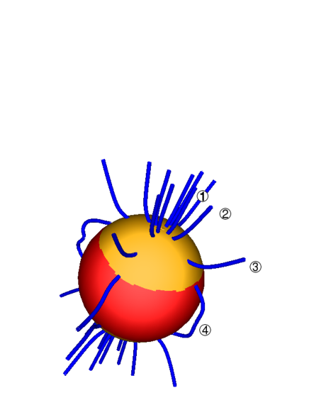
Figure 10: Magnetic pitch angle $B_{\phi}/B_{p}$ (right panel) as a function of the coordinate $\eta$ along four magnetic field lines 1–4 for model D, for a snapshot taken at $t=5\tau_{\mathrm{A}}$. The positions of the field lines are depicted in the left panel. The mountain is defined by the orange isosurface $\rho(r,\theta,\phi)=1.04\times 10^{9}$ g cm³, while red denotes the neutron star surface $r=R_{\ast}$. In order to improve visibility, all length scales of the mountain and the field lines (blue) are magnified five-fold.

The concept of rational magnetic surfaces, where the field lines close upon themselves, plays an important role in a local plasma stability analysis. The bending of field lines as a result of a Lagrangian displacement is associated with an increase in potential energy. Hence, for almost all instabilities to occur, this contribution, which can be expressed as $\mathbf{B}\mn@boldsymbol{\cdot}\nabla\mn@boldsymbol{\xi}$, needs to be small. In a tokamak geometry, it can be shown that this term vanishes on a rational surface. The spatial location of rational surfaces is directly related to the pitch angle $B_{\phi}/B_{p}$. We defer a detailed analysis of the rational magnetic surfaces in our problem to a forthcoming paper and restrict ourselves to a brief discussion in the following paragraph.

In Fig. 10, we plot the pitch angle as a function of the coordinate $\eta$ along the field line (right panel) for four different field lines (left panel) in model D. We first note that the toroidal component stays below 20 per cent of the poloidal component along all four field lines. Furthermore, the absolute magnitude of the pitch angle tends to increase with colatitude. This is consistent with the previous discussion. The Parker instability (and hence $B_{\phi}$) dominates close to the magnetic equator. The wave-like character of the instability is vividly demonstrated by the zero crossings of the pitch angle.

4.2 Mass and magnetic quadrupole moments

Figure 11: Mass quadrupole moments for model D, normalised to the maximum of $Q_{33}$ ($1.30\times 10^{25}$ g cm²) as a function of time in units of the Alfvén time. The sytem develops a substantial asymmetry, characterised by the off-diagonal element $Q_{12}$, during the relaxation phase, before settling down to a nearly axisymmetric state.

At $t\approx 2\tau_{\mathrm{A}}$, the system in Fig. 7 settles down to a stable state which differs from the initial configuration, primarily by being nonaxisymmetric with respect to the pre-accretion magnetic axis. The field lines whose footpoints are at a low colatitude move towards the magnetic poles. This behaviour is reflected in the mass quadrupole moments, plotted against time in Fig. 11. The transition to a nonaxisymmetric magnetic field configuration at $t\approx\tau_{A}$ is accompanied by a sudden rise in the off-diagonal moment $Q_{12}$. However, by the time the mountain settles down at $t\approx 2\tau_{A}$, axisymmetry is largely restored and $Q_{12}$ decreases. Fig. 11 shows that $Q_{12}$ oscillates before damping down, with a remarkably low deviation from axisymmetry of $Q_{12}/Q_{33}<0.1$ per cent in the final state.

We reiterate that the final state is not the same as the initial state, even though it is nearly axisymmetric. Furthermore, the final state is stable. This is the main result of the paper, as far as astrophysical applications are concerned.

Figure 12: Meridional section for model D at $t/\tau_{A}=0,1,2,3,4,5$ (top left to bottom right). Shown are the density contours (dashed curves) for $\log_{10}(\rho/\rho_{0}^{\prime})=-13,-12,-11,-10.7,-10.5,-10.3$, and the normalised Lorentz force per unit volume $(\mathbf{J}\times\mathbf{B})_{\phi}/|\mathbf{J}\times\mathbf{B}|$ (solid curves) for the values 0.1, 0.5, 0.9. The Lorentz force develops a toroidal component as $B_{\phi}$ increases, but its poloidal component diminishes, allowing the poloidal pressure gradient to push the mountain equatorwards.

Why does $Q_{ij}$ decrease? Naively, one would not expect a significant change, given that the Parker instability predominantly acts in the equatorial belt region, while most of the plasma is located at the magnetic pole. The answer can be found in the Lorentz force, which balances the lateral pressure gradient. Fig. 12 shows how the relative strength of the toroidal component of the Lorentz force, $(\mathbf{J}\times\mathbf{B})_{\phi}/|\mathbf{J}\times\mathbf{B}|$ (dashed curve), grows as a function of time in model D. As $B_{\phi}$ grows, following the onset of the instability, the force per unit volume develops a toroidal component while its lateral component decreases. Hence the (approximately unchanged) lateral hydrostatic pressure gradient forces the mountain to slip towards the equator. After the system settles down, $B_{\phi}$ decreases and the lateral components of $\mathbf{J}\times\mathbf{B}$ and $\nabla p$ readjust to balance each other, leading to the stable equilibrium state.

The ellipticity $\epsilon\propto Q_{22}$ reaches a local maximum during the transition phase at $t\approx\tau_{A}$ and subsequently drops. The mass quadrupole moment of the final configuration is $\approx 33$ per cent lower than in model A. The asymptotic values of $Q_{ij}$ for the eight models in Table 1 are tabulated in Table 2, normalized to $Q_{33}(t=8\tau_{\mathrm{A}})$ for model A.

Table 2: Asymptotic values of $Q_{ij}$ for the eight models in Table 1, normalized to $\hat{Q}_{33}=Q_{33}(t=8\tau_{\mathrm{A}})$ for model A. We select $t=8\tau_{\mathrm{A}}$ (models A–E), $t=5\tau_{\mathrm{A}}$ (models F & G), and $t=4\tau_{\mathrm{A}}$ (models J & K) to compute the asymptotic value.

Model	$Q_{12}/\hat{Q}_{33}$	$Q_{22}/\hat{Q}_{33}$	$Q_{33}/\hat{Q}_{33}$
A	$-3.1\times 10^{-8}$	$-0.50$	$1.00$
B	$-3.1\times 10^{-8}$	$-0.51$	$1.02$
D	$1.6\times 10^{-3}$	$-0.21$	$0.64$
E	$-3.1\times 10^{-8}$	$-0.51$	$1.02$
F	$-1.9\times 10^{-3}$	$-0.23$	$0.60$
G	$8.7\times 10^{-4}$	$-0.17$	$0.68$
J	$5.7\times 10^{-2}$	$-1.27$	$3.9$
K	$2.5\times 10^{-4}$	$-4.72$	$12$

Figure 13: Magnetic dipole moment $d_{10}/R_{m}^{3}$ (bottom) and magnetic quadrupole moment $d_{21}/R_{m}^{4}$ (top, middle) for model D, normalised to the initial value of $d_{10}/R_{m}^{3}=5.29\times 10^{-7}B_{0}$, as a function of time (in units of the Alfvén time scale). All other components vanish due to symmetry.

The nonvanishing components of the magnetic dipole and quadrupole moments $d_{lm}(r=R_{m})$, defined as

$$d_{lm}(r=R_{m})=R_{m}^{l+2}\int\mathrm{d}\Omega\;Y_{lm}^{\ast}B_{r}$$ (9)

(see appendix C), are displayed as functions of time in Fig. 11. The dipole moment $d_{10}=4(\pi/3)^{1/2}\mu$ increases rapidly during the transition phase, reaching an asymptotic maximum of 5.5 times the initial value. Likewise, the quadrupole $d_{21}$ peaks during the transition phase before settling down to a constant value. The final field is highly axisymmetric, deviating from perfect symmetry by $|d_{21}|R_{m}/d_{10}=0.8$ per cent. The asymptotic values of $d_{lm}$ for models A–K are listed in Table 3.

Table 3: Non-vanishing components of the asymptotic magnetic dipole moments $d_{10}/R_{m}^{3}$ and magnetic quadrupole moments $q_{10}/R_{m}^{4}$, both normalised to $\hat{d}_{10}/R_{m}^{3}=d_{10}(t=8\tau_{\mathrm{A}})/R_{m}^{3}$. We select $t=8\tau_{\mathrm{A}}$ (models A–E), $t=5\tau_{\mathrm{A}}$ (models F & G), and $t=4\tau_{\mathrm{A}}$ (models J & K) to compute the asymptotic value.

Model	$d_{10}/\hat{d}_{10}$	$\mathrm{Re}(d_{21})/(\hat{d}_{10}R_{m})$	$\mathrm{Im}(d_{21})/(\hat{d}_{10}R_{m})$
A	$1.0$	$-4.6\times 10^{-8}$	$-4.8\times 10^{-9}$
B	$1.3$	$-5.9\times 10^{-8}$	$-6.1\times 10^{-9}$
D	$7.4$	$4.8\times 10^{-2}$	$-4.3\times 10^{-2}$
E	$1.3$	$-5.9\times 10^{-8}$	$-6.1\times 10^{-9}$
F	$7.3$	$1.1\times 10^{-1}$	$8.2\times 10^{-3}$
G	$7.1$	$2.1\times 10^{-2}$	$-5.5\times 10^{-2}$
J	$21$	$-1.2$	$-0.12$
K	$57$	$-6.3\times 10^{-4}$	$9.1\times 10^{-4}$

4.3 Boundary conditions

Figure 14: Meridional section of density contours (left) and magnetic field lines (right) for model D (solid curve) and model E (dotted curve). The inflow boundary condition corresponds to line-tying at the outer boundary. Deviations between the two models occur in the outermost, low density regions.

We perform a simulation (model E) with the same initial configuration as model D ($M_{a}/M_{c}=1.0$ and $b=3$) but with inflow boundary conditions at $R=R_{m}$. Fig. 14 compares the density (left panel) and magnetic field (right panel) of models D and E. Again, inflow pins the magnetic field at the outer boundary, as opposed to outflow, which leaves the field free. The density distribution is almost unaffected. The magnetic field is mainly affected in the outermost region, where the plasma density is low. The overall time evolution (a nonaxisymmetric transition phase which leads to a nearly axisymmetric equilibrium) remains as before, too. We therefore conclude that the outer boundary condition can be chosen opportunistically.

By contrast, the inner boundary condition contributes fundamentally to stability. The tension of the magnetic field, which is tied to the stellar surface, suppresses those modes which are driven by a pressure gradient perpendicular to the magnetic flux surfaces, such as the interchange and ballooning mode. If line-tying is taken away, the latter modes disrupt the mountain in short order. If we rerun model A (for example) by applying a reflecting boundary condition at $r=R_{\ast}$, the mountain rapidly dissolves on a timescale $\sim\tau_{0}$. The same experiment for model D results in high velocities and steep field gradients, causing the numerical algorithm of zeus-mp to break down.

4.4 Energetics

Mouschovias (1974) showed that an isothermal, gravitating, MHD system possesses a total energy $W$, which can be written as the sum of gravitational, kinetic, magnetic, and acoustic contributions, defined by the following volume integrals, evaluated over the simulation volume:

$$W_{\mathrm{g}}=\int\mathrm{d}V\rho\varphi,$$ (10)

$$W_{\mathrm{k}}=\frac{1}{2}\int\mathrm{d}V\rho v^{2},$$ (11)

$$W_{\mathrm{m}}=\frac{1}{2\mu_{0}}\int\mathrm{d}VB^{2},$$ (12)

$$W_{\mathrm{a}}=\int\mathrm{d}Vp\log p.$$ (13)

Here, $\mathbf{v}$ is the plasma velocity and $p=c_{s}^{2}\rho$ is the pressure.

Figure 15: The evolution of the total energy $W$ and its components $W_{\mathrm{m}}$, $W_{\mathrm{g}}$, $W_{\mathrm{k}}$, and $W_{\mathrm{a}}$ (top to bottom) for model D, all normalised to $W_{0}=2.2\times 10^{36}$ erg, as a function of time (in units of the Alfvén time scale). The total energy increases artifically, due to mass loss through the outer boundary (see text).

The evolution of (10)–(13) for model D is shown in Fig. 15. The magnetic energy (second panel from top) steadily decreases to $20$ per cent of its original value, as the axisymmetric equilibrium evolves to a lower energy, nonaxisymmetric state. The kinetic energy peaks at $t=1.2\tau_{A}$, during the transition phase when the magnetic reconfiguration occurs. However, the gravitational and acoustic contributions, which dominate $W$, increase with time. The reason for this becomes apparent if we track the total mass in the simulation volume. Approximately 3.7 per cent of the mass is lost through the outflow boundary at $r=R_{m}$ by $t=6\tau_{\mathrm{A}}$. The mass loss is responsible for the increase of $W_{\mathrm{a}}\propto\rho^{2}$ and $W_{\mathrm{g}}\propto\rho$, both of which are negative ($W_{\mathrm{g}}$ because the plasma is gravitationally bound and $W_{\mathrm{a}}$ since $\rho<1$ in our units).

Figure 16: The evolution of the total energy $W$ and its components $W_{\mathrm{m}}$, $W_{\mathrm{g}}$, $W_{\mathrm{k}}$, and $W_{\mathrm{a}}$ (top to bottom) for model D, all normalised to $W_{0}=2.2\times 10^{36}$ erg, as a function of time (in units of the Alfvén time scale). $W$, $W_{\mathrm{g}}$, and $W_{\mathrm{a}}$ are now corrected for the mass loss through the outer boundary (cf. Fig. 15).

Let us try to correct for the mass loss by multiplying $W_{g}$, $W_{k}$, and $W_{a}$ by $M(t=0)/M(t)$, where $M(t)$ is the mass in the simulation volume at time $t$. The result is presented in Fig. 16. $W_{g}$ and $W_{a}$ now decrease, and the total energy, $W=W_{\mathrm{g}}+W_{\mathrm{k}}+W_{\mathrm{m}}+W_{\mathrm{a}}$, decreases by just 2.5 per cent.

Figure 17: The evolution of the total energy $W$ and its components $W_{\mathrm{m}}$, $W_{\mathrm{g}}$, $W_{\mathrm{k}}$, and $W_{\mathrm{a}}$ (top to bottom) for model E, all normalised to $W_{0}=2.2\times 10^{36}$ erg, as a function of time (in units of the Alfvén time scale).

The approximate correction above assumes $\rho$ decreases uniformly, which is not strictly true. We therefore check our claim that mass loss is responsible by tracking the energy evolution of model E, which has the same initial configuration as model D, but an inflow outer boundary which blocks mass loss. From Fig. 17, it is clear that the total energy rises then falls, consistent with the observed dynamical evolution. The mountain oscillates until toroidal modes grow sufficiently to disrupt the initial configuration and force it into a nonaxisymmetric state. There is no spurious increase in $W$. We conclude that mass loss through the outer boundary is indeed responsible for the observed behaviour of $W$ in model D in Fig. 15.

4.5 Dependence on $M_{a}$

Figure 18: The mass quadrupole moments for models F (solid), D (dotted), and G (dashed), normalised to $1.33\times 10^{25}$ g cm², as a function of time. While all models show similar dynamical behaviour, the quadrupole moment of the final state increases with $M_{a}$.

Does the final, nonaxisymmetric configuration of the mountain become unstable once the accreted mass exceeds a critical threshold? There are two ways that this can happen. First, the sequence of nonaxisymmetric GS equilibria passed through as $M_{a}$ increases can terminate above a critical value of $M_{a}$; i.e. there is a loss of equilibrium. PM07 observed this phenomenon in axisymmetric magnetic mountains with $M_{a}\ga 10^{-4}M_{\odot}$, when the source term in the GS equation forces the flux function outside the range $0\leq\psi\leq\psi_{\ast}$ permitted by the boundary condition at $r=R_{\ast}$. Second, the nonaxisymmetric state reached in Fig. 7 (for example) may be metastable. That is, it may be a local energy minimum which can be reached from an axisymmetric starting point via the Parker instability but which the system can exit (in favor of some other, global energy minimum) if the system is kicked hard enough. One way to kick the system hard is to increase $M_{a}$ substantially.

We are not really in a position to answer this question definitively, because the GS fails to converge to valid equilibria for $M_{a}\gg 10^{-4}M_{\odot}$, due to numerical difficulties (steep gradients, which would be smoothed in a more realistic, non-ideal-MHD simulation). Nevertheless, we begin to address the issue by performing two simulations, models F and G, with the same parameters as model D but with lower and higher masses viz. $M_{a}/M_{c}=0.6$ and $M_{a}/M_{c}=1.4$ respectively. The mass quadrupole moments are plotted versus time in Fig. 18. The solid and dashed curves are for models F and G respectively, with model D (dotted curve) overplotted for comparison.

The dynamical behaviour of all three models is similar: a violent transition phase which settles down to a nonaxisymmetric state. However, the start of the transition phase, defined as the instant where $Q_{33}$ is maximized, scales roughly $\propto 0.5M_{a}/M_{c}$ in units of $\tau_{A}$. Physically, this means that the onset of the toroidal instability depends on $M_{a}$. We can understand the trend in terms of the Parker instability (section 4.1), whose growth rate scales as $\Gamma_{\mathrm{P}}\propto v_{\mathrm{A}}^{-1}$. By measuring $v_{A}$ at $\theta=\pi/2$ in models D,F, and G, we find $v_{A}\propto M_{a}$ empirically and $\Gamma_{\mathrm{P}}\propto M_{a}^{-1}$, consistent with the Parker scalings.

Figure 19: Ellipticity $\epsilon$ for models F (solid), D (dotted), and G (dashed) as a function of time. As expected, $\epsilon$ increases with $M_{a}$.

The evolution of the ellipticity $\epsilon\propto Q_{33}$ for models D, F, and G is displayed in Fig. 19. Of chief interest here is the ellipticity of the final state. It increases along with $M_{a}$, consistent with Melatos & Payne (2005). A linear fit yields the following rule of thumb for our downscaled star (section 2.3):

$$\frac{\epsilon}{10^{-10}}=1.12\frac{M_{a}}{M_{c}}.$$ (14)

Note, however, that the fit is valid in the range $0.6\leq M_{a}/M_{c}\leq 1.4$. Numerical difficulties prevent us from extending it to larger values of $M_{a}$. Payne & Melatos (2006a) found $\epsilon/10^{-10}=7.8M_{a}/M_{c}(1+1.1M_{a}/M_{c})^{-1}$ in the $M_{a}\sim M_{c}$ regime for the axisymmetric equilibrium. Equation (14) yields values roughly 70 per cent lower than the latter formula.

Figure 20: Azimuthal magnetic field component $|B_{\phi}|$ for models F (solid), D (dotted), and G (dashed), in units of $B_{0}$, plotted as a function of time, in units of the Alfvén time.

For completeness, we plot the magnitude of the toroidal field component $|B_{\phi}|$ versus time in Fig. 20. Interestingly, the peak value is achieved for the intermediate mass model, D, not for model G. However, $B_{\phi}$ in the final state depends weakly on $M_{a}$. We find $B_{\phi,\mathrm{F}}=3.4\times 10^{-7}B_{0}$, $B_{\phi,\mathrm{D}}=4.5\times 10^{-7}B_{0}$, and $B_{\phi,\mathrm{G}}=3.2\times 10^{-7}B_{0}$, where $B_{0}$ is defined in section 2.3. These values are comparable to the magnitude of the polar magnetic field $B_{\mathrm{p}}=2.9\times 10^{-7}B_{0}$.

4.6 Dependence on curvature

As discussed in section 2.3, PM07 argued that reducing $R_{\ast}$ and $M_{\ast}$ does not affect the equilibrium structure as long as $h_{0}$ remains constant, at least in the small-$M_{a}$ limit. To test whether this also holds for the dynamical behaviour of the system, we perform two runs, models J and K, with $a=75$ and $a=100$ respectively.

Figure 21: Mass quadrupole moments $Q_{ij}$ for model J ($a=75$, solid curve) and model K ($a=100$, dashed curve), plotted as a function of time (in units of the Alfvén time). The scale for model J (K) appears on the left (right) vertical axis. Although the transition phase is less distinct than in Fig. 11, these models basically share the same dynamics as lower curvature runs.

Fig. 21 plots $Q_{ij}$ versus time for these models. The transition phase is more gradual than model D (Fig. 11). Again, however, $Q_{12}$ rises significantly, marking a deviation from axisymmetry. Melatos & Payne (2005) found $\epsilon\propto a^{2}$ analytically in the small-$M_{a}$ regime, so we fit a parabola to the simulation data (for $M_{a}=M_{c}$):

$$\frac{\epsilon}{10^{-13}}=1.82a^{2}.$$ (15)

A realistic star has $a=1.9\times 10^{4}$ (cf. section 2.3). Extrapolating (15), we find $\epsilon=6.6\times 10^{-5}$. (An ellipticity this large is close to the upper limit inferred from existing gravitational-wave nondetections; see section 6 for more details.) However, it should be remembered that equation (15) is an overestimate, because the computations in this paper neglect nonideal MHD effects.

5 Global MHD oscillations

In this section, we explore the natural oscillation modes of a nonaxisymmetric magnetic mountain. We do this by loading the final state from models D, F, and G into zeus-mp and setting $\mathbf{v}=0$ on the whole grid. This procedure introduces numerical perturbations that are sufficient to excite small linear oscillation modes, albeit an uncontrolled distribution thereof. We then compute the power spectrum

$$P[S](\omega)=\left|\frac{1}{N}\sum_{i=0}^{N-1}S(t_{i})\mathrm{e}^{-i\omega t_{i}/N}\right|^{2}$$ (16)

by evaluating the discrete Fourier transform of the scalar function $S(t)$ [e.g. $B_{r}(t)$] at $N$ sample times $t_{i}$.

In order to explore the magnetic modes, we examine $B_{r}$, $B_{\theta}$, and $B_{\phi}$. We choose one point on the grid where the amplitude of the oscillations is high, namely $(r,\theta,\phi)=(50.03h_{0},0.26,2.06)$ and compute $P[B_{r}]$, $P[B_{\theta}]$, and $P[B_{\phi}]$. The results are displayed in Fig. 22. We can distinguish five different spectral peaks at $10^{3}\omega\tau_{0}=0.78,1.1,1.2,2.1,3.2$, which are more or less distinct for the different components.

Figure 22: Power spectrum of $B_{r}$, $B_{\theta}$, and $B_{\phi}$ (top to bottom) for model D (arbitrary units), plotted as a function of angular Fourier frequency (in units of $\tau_{0}^{-1}$).

For a magnetized gravitating slab in a plane-parallel geometry, one can distinguish three different MHD modes (Goedbloed & Poedts, 2004): slow magnetosonic, Alfvén, and fast magnetosonic. Each mode consists of a discrete set of eigenmodes and a continuous spectrum, which are clearly separated. Unfortunately, such clean separation cannot be expected for a highly inhomogenous plasma in spherical geometry. Generally, different parts of the spectrum overlap or degenerate into a single point in a nontrivial way. We therefore restrict the discussion below to some qualitative remarks.

The MHD spectrum contains genuine singularities, when the eigenfrequency coincides with the Alfvén or slow magneto-sonic frequency at some location within the magnetic mountain. In this case, the boundary value problem becomes singular; the boundary conditions can be fulfilled for a continuous range of frequencies. The singular frequencies depend on the components of the wave vector perpendicular to the direction of inhomogenity.

It is unclear whether the band $\omega<0.002\tau_{0}^{-1}$, which looks “filled” in Fig. 22, belongs to the continuous part of the spectrum or else is an artifact of the nonzero line width from numerical damping (which can be estimated from the sample times $t_{i}$ to be $\sim 1.2\times 10^{-4}\omega\tau_{0}$). We do not observe any singular behaviour in the field variables, but we note that singularities would be suppressed by the shock-capturing algorithm (i.e. the artificial viscosity) in zeus-mp. We conclude that the features in Fig. 22 are probably discrete lines.

Figure 23: Power spectra of $B_{r}$ and $B_{\theta}$ (top to bottom) for model A (arbitrary units), plotted as a function of angular Fourier frequency (in units of $\tau_{0}^{-1}$).

Let us compare these results to the spectrum of the axisymmetric model A (Fig. 23). We first note that the Alfvén frequency $\omega_{A}=0.018\tau_{0}^{-1}(M_{a}/M_{c})^{-1/2}$ and acoustic frequency $\omega_{s}=0.48\tau_{0}^{-1}$ found by PM07 are outside the range of this plot, which is set by the Nyquist frequency $\omega_{\mathrm{N}}=(4\pi N\Delta t)^{-1}$ ($\Delta t=50\tau_{0}$ for model A and $\Delta t=10\tau_{0}$ for models D–G). Here, we are restricted to low frequency oscillations which are generally associated with global magnetic modes. Most distinct is the peak at $10^{3}\omega\tau_{0}=0.5$, which is not visible in Fig. 22. This long wavelength poloidal mode is suppressed in favor of toroidal modes in the three-dimensional configuration. However, the small peak at $10^{3}\omega\tau_{0}=1.1$ is present in both systems. This example illustrates vividly how relaxing the axisymmetric constraint leads to a different MHD spectrum.

Figure 24: Power spectra of $B_{r}$, $B_{\theta}$, and $B_{\phi}$ (top to bottom) for models F (solid curve) and G (dashed curve) in arbitrary units, plotted as a function of angular Fourier frequency in units of $\tau_{0}^{-1}$. We overplot the spectrum of model G, stretched by a factor of 1.4 in $\omega$, as dotted curve, by way of comparison.

Fig. 24 shows the power spectrum for models F (solid) and G (dashed). The most distinct peaks are again concentrated in the low frequency region. We can roughly match the peaks of models G and F by stretching the former spectrum by a factor of 1.4 in frequency. The higher $M_{a}$ equilibrium has a similar structure, but the Alfvén timescale is lower because the plasma density is 85 per cent higher.

A complete analytic determination of the discrete and continuous components of the MHD spectrum via a full linear mode analysis will be attemped in a forthcoming paper.

6 Discussion

Magnetically confined mountains on accreting neutron stars screen the magnetic dipole moment of the star. Potentially, therefore, the process of polar magnetic burial can explain the observed reduction of $\mu$ with $M_{a}$ in neutron stars with an accretion history. However, before magnetic burial can be invoked as a viable explanation, the question of stability must be resolved. In this article, we concentrate on the important aspect of three-dimensional stability, deferring resistive processes to future work (especially the issue of resistive g-modes).

We find that the axisymmetric configurations in PM04 are susceptible to the three-dimensional magnetic buoyancy instability. The instability proceeds via the undular submode, with growth rate $\propto\lambda^{1/2}$, limited by the toroidal grid resolution. However, instead of breaking up and reverting to an isothermal atmosphere threaded by a dipolar magnetic field, the magnetic field reconfigures (over a few Alfvén times) and settles down into a new nonaxisymmetric equilibrium which is still highly distorted. Just as the axisymmetric solutions in PM04 are the final saturated states of the nonlinear evolution of the Parker instability in two dimensions, we find here the three-dimensional equivalent. This surprising result is the main conclusion of the paper. It holds irrespective of the outer boundary condition and curvature rescaling factor, but it depends critically on the line-tying boundary condition at the stellar surface.

The final state is predominantly axisymmetric, with $1.5\leq|Q_{12}/Q_{33}|/10^{-3}\leq 3.2$ for models D, F, and G ($0.6\leq M_{a}/M_{c}\leq 1.4$). The ellipticity for model G reaches $1.6\times 10^{-10}$ in the downscaled star.

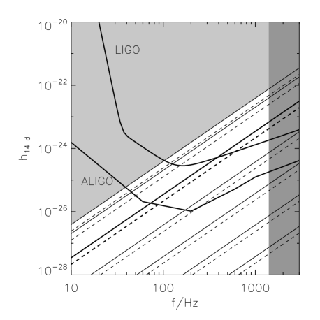
Figure 25: Amplitude of the gravitational wave signal $h_{0}$ for $M_{a}/M_{\odot}=10^{-9},10^{-8},10^{-7},10^{-6},10^{-5},10^{-4},10^{-3}$, for the axisymmetric (solid lines) and nonaxisymmetric equilibrium (dashed lines). The sensitivities of Initial and Advanced LIGO, assuming 14 days coherent integration, are also plotted (upper and lower curves respectively). The growth of the mountain is arrested for $M_{a}\ga 1.2\times 10^{-5}M_{\odot}$ (light shaded region), due to Ohmic dissipation (Melatos & Payne, 2005; Vigelius & Melatos, 2008), while the right-hand edge is excluded at present because no accreting millisecond pulsars have been discovered with $f_{\ast}>0.7$ kHz (dark shaded region).

The stability of magnetic mountains is important for the emission of gravitational waves from accreting millisecond pulsars, as pointed out previously by Melatos & Payne (2005). Persistent X-ray pulsations from accreting binary pulsars imply that the angle between the spin vector $\mathbf{\Omega}$ and the magnetic symmetry axis $\mn@boldsymbol{\mu}$ is not zero (Romanova et al., 2004; Kulkarni & Romanova, 2005). Hence a magnetic mountain constitutes a time-varying mass quadrupole which emits gravitational waves. Furthermore, the star precesses in general, emitting gravitational waves at the spin frequency and its first harmonic. The amplitude of the resulting signal (with curvature upscaled to a realistic neutron star at a distance $d=10$ kpc using $\epsilon\propto a^{2}$) is plotted in Fig. 25 for $10^{-9}\leq M_{a}/M_{\odot}\leq 10^{-3}$. The amplitude of the average signal that can be detected by the Laser Interferometer Gravitational Wave Observatory (LIGO) from a periodic source with a false alarm rate of 1 per cent and a false dismissal rate of 10 per cent over an integration time of $T_{0}=14$ days (Jaranowski et al., 1998; Abbott, B. et al., 2004), is overplotted in Fig. 25. This $T_{0}$ can realistically be achieved computationally.

At this point, it is important to acknowledge that $M_{a}=1.4M_{c}\approx 1.7\times 10^{-4}M_{\odot}$ is still well below $M_{a}\sim 0.1M_{\odot}$, the mass required to spin up a neutron star to millisecond periods (Burderi et al., 1999). At present, this high-mass regime is not accessible numerically; neither the GS solver nor zeus-mp can handle the steep magnetic gradients involved. By the same token, Ohmic diffusion becomes important in this high-$M_{a}$ regime (Melatos & Payne, 2005; Vigelius & Melatos, 2008), smoothing the gradients and mitigating the numerical challenge. We postpone studying realistic values of $M_{a}$ to an accompanying paper, which will concentrate on non-ideal MHD simulations. However, to make a rough estimate regarding detectability here, we assume that non-ideal effects stall the growth of the mountain at $M_{a}\approx M_{c}$, following Melatos & Payne (2005). This includes the region shaded light grey in Fig. 25. Furthermore, no accreting millisecond pulsars have been discovered spinning faster than $f_{\ast}\ga 720$ Hz, possibly due to braking by gravitational waves (Bildsten, 1998; Chakrabarty et al., 2003). The region with $2f_{\ast}\ga 1400$ Hz is shaded dark grey in Fig. 25.

Even with those exclusions, Fig. 25 demonstrates that there is a fair prospect of detecting gravitational waves from accreting X-ray millisecond pulsars in the near future, for accreted masses as low as $M_{a}\approx 10^{-4}M_{\odot}$. Recent directed searches for gravitational waves from the nearby X-ray source Sco-X1 found no signal at the level $h_{0}\ga 10^{-22}$ (Abbott, B. et al., 2007), thereby setting an upper bound on the ellipticity of $\epsilon=3.6\times 10^{-3}$.

Appendix A Defining the grid and boundary conditions in zeus-mp

In this appendix, we briefly outline the key variables and settings in zeus-mp, to aid the reader in reproducing our numerical results. Our grid consists of ggen1:nbxl, ggen2:nbxl, and ggen3:nbxl blocks in the $r$, $\theta$, and $\phi$ direction, respectively. The integration volume is defined by $R_{\ast}/h_{0}\leq r\leq R_{m}$, $0\leq\theta\leq\pi/2$, $0\leq\phi<2\pi$. The radial coordinate in the GS code, $\tilde{x}=(r-R_{\ast})/h_{0}$ ($0\leq\tilde{x}\leq X$), is stretched logarithmically according to $\tilde{x}_{1}=\log(\tilde{x}+\mathrm{e}^{-L_{x}})+L_{x}$, where $L_{x}$ controls the zooming (PM04). This grid is implemented by setting the zeus-mp parameters $\mathtt{ggen1:x1min}=R_{\ast}/h_{0}$ and $\mathtt{ggen1:x1max}=\mathtt{ggen1:x1min}+X$. Stretching is achieved via the parameter ggen1:x1rat, which sets the radial length ratio of two neighbouring zones. In order to get consistent radial grid positions in the GS code and zeus-mp, we set $\mathtt{ggen1:x1rat}=(X\mathrm{e}^{L_{x}}+1)^{(G_{x}-1)^{-1}}$.

Boundary conditions are enforced in zeus-mp via ghost cells, which frame the active grid cells. Several predefined prescriptions are supplied to implement a variety of standard boundary conditions. In the $\phi$ direction, we choose periodic boundary conditions [ikb.niks(1)=4 and okb.noks(1)=4]. The $\theta=\pi/2$ surface is reflecting, with normal magnetic field [ojb.nojs(1)= 5], which translates to $\mathbf{v}_{\perp}=\mathbf{B}_{\parallel}=0$. The line $\theta=0$ is also reflecting [ijb.nijs(1)= -1] with tangential magnetic field ($\mathbf{v}_{\perp}=\mathbf{B}_{\perp}=0$). Additionally, the toroidal component $B_{\phi}$ is reversed at the boundary, i.e. $B^{<}_{\phi}=-B^{>}_{\phi}$, where $B_{\phi}^{<}$ and $B_{\phi}^{>}$ are the field components for $\theta<0$ and $\theta>0$, respectively. The outer surface $r=R_{m}$ is usually an outflow [oib nois(1)= 2] boundary, i.e. zero gradient. The stellar surface is impenetrable, so the inner $r=R_{\ast}$ boundary is inflow [iib.niis(1)= 3]. This enables us to impose line-tying at $r=R_{\ast}$ by fixing the density and magnetic field there. We also use an isothermal equation of state (XISO=.true.).

Appendix B Mass multipole moments

We work out the mass quadrupole moment in Cartesian coordinates from the code output in spherical coordinates. Following Jackson (1998), we define the spherical mass multipole moments according to

$$q_{lm}=\int\mathrm{d}^{3}\mathbf{x^{\prime}}Y^{*}_{lm}(\theta^{\prime},\phi^{\prime})r^{\prime l}\rho(\mathbf{x}^{\prime}),$$ (17)

where $Y_{lm}$ denotes the usual orthonormal set of spherical harmonics.

The spherical quadrupole moments are related to the traceless, Cartesian quadrupole moment tensor,

$$Q_{ij}=\int d^{3}x^{\prime}\,(3x_{i}^{\prime}x_{j}^{\prime}-r^{\prime 2}\delta_{ij})\rho(\mathbf{x^{\prime}}),$$ (18)

by $Q_{11}=6(2\pi/15)^{1/2}\mathrm{Re}(q_{22})-2(4\pi/5)^{1/2}q_{20}$, $Q_{12}=-6(2\pi/15)^{1/2}\mathrm{Im}(q_{22})$, $Q_{13}=-3(8\pi/15)^{1/2}\mathrm{Re}(q_{21})$, $Q_{22}=-6(2\pi/15)^{1/2}\mathrm{Re}(q_{22})-(4\pi/5)^{1/2}q_{20}$, and $Q_{23}=3(8\pi/15)^{1/2}\mathrm{Im}(q_{21})$.

In the axisymmetric case (when the star and the mountain form a prolate spheroid), we have $\rho=\rho(r,\theta)$ and the $\phi$ integrals in (17) vanish. $Q$ is then diagonal with components $Q_{\hat{x}\hat{x}}=Q_{\hat{y}\hat{y}}=-Q_{\hat{z}\hat{z}}/2$, with respect to the body coordinate system, and we can introduce the ellipticity $\epsilon$, where we assume that the $\hat{z}$ axis is the symmetry axis:

$$\epsilon=\frac{Q_{\hat{z}\hat{z}}}{2I_{\hat{z}\hat{z}}}=\frac{3(I_{\hat{z}\hat{z}}-I_{\hat{x}\hat{x}})}{I_{\hat{z}\hat{z}}},$$ (19)

with $I_{\hat{z}\hat{z}}=2M_{\ast}R_{\ast}^{2}/5$ is the moment of inertia along the rotation axis for a biaxial ellipsoid with mass $M_{\ast}$ and minor axis $R_{\ast}$. We can compute the ellipticity directly from the code output through

$$\epsilon=\frac{1}{2I_{\hat{z}\hat{z}}}\int d\theta\,d\phi\,dr\,\rho r^{4}\sin\theta(3\cos^{2}\theta-1).$$ (20)

Appendix C Magnetic multipole moments

In a source-free region $\mathbf{J}=0$, a magnetic field $\mathbf{B}$ is determined solely by its radial component $B_{r}$ (Bouwkamp & Casimir, 1954), which, from Maxwell’s equations, satisfies the Laplace equation

$$\nabla^{2}B_{r}=0.$$ (21)

One can therefore define the magnetic multipoles as the expansion coefficients in the general solution of the boundary value problem (21), viz.

$$B_{r}=\sum_{l=0}^{\infty}\sum_{m=-l}^{l}d_{lm}r^{-(l+1)}Y_{lm}(\theta,\phi),$$ (22)

with

$$d_{lm}=r^{l+1}\int\mathrm{d}\Omega\;Y_{lm}^{\ast}\mathbf{r}\mn@boldsymbol{\cdot}\mathbf{B}.$$ (23)

Note that $d_{10}$ is related to the magnetic moment $\mu$ of a dipole field $\mathbf{B}(\mathbf{r})=\mu r^{-3}(2\cos\theta\mathbf{e}_{r}+\sin\theta\mathbf{e}_{\theta})$ by $d_{10}=4(\pi/3)^{1/2}\mu$.

In the case of north-south symmetry, we find $d_{10}=2\hat{d}_{10}$ and $d_{21}=2\hat{d}_{21}$, where a hat denotes the moment evaluated on the hemisphere. All other coefficients vanish.

References

- Abbott, B. et al. (2004) Abbott, B. et al. 2004, Phys. Rev. D, 69, 082004
- Abbott, B. et al. (2007) Abbott, B. et al. 2007, Phys. Rev. D, 76, 082001
- Akiyama et al. (2003) Akiyama S., Wheeler J. C., Meier D. L., Lichtenstadt I., 2003, ApJ, 584, 954
- Balbus & Hawley (1998) Balbus S. A., Hawley J. F., 1998, Rev. Mod. Phys., 70, 1
- Bildsten (1998) Bildsten L., 1998, ApJ, 501, L89+
- Biskamp (1993) Biskamp D., 1993, Nonlinear magnetohydrodynamics. Cambridge University Press, Cambridge.
- Bisnovatyi-Kogan & Komberg (1974) Bisnovatyi-Kogan G. S., Komberg B. V., 1974, Soviet Astronomy, 18, 217
- Bonazzola & Gourgoulhon (1996) Bonazzola S., Gourgoulhon E., 1996, A&A, 312, 675
- Bouwkamp & Casimir (1954) Bouwkamp C. J., Casimir H. B. G., 1954, Physica, 20, 539
- Brown & Bildsten (1998) Brown E. F., Bildsten L., 1998, ApJ, 496, 915
- Burderi et al. (1999) Burderi L., Possenti A., Colpi M., di Salvo T., D’Amico N., 1999, ApJ, 519, 285
- Chakrabarty et al. (2003) Chakrabarty D., Morgan E. H., Muno M. P., Galloway D. K., Wijnands R., van der Klis M., Markwardt C. B., 2003, Nature, 424, 42
- Cumming et al. (2004) Cumming A., Arras P., Zweibel E., 2004, ApJ, 609, 999
- Cutler (2002) Cutler C., 2002, Phys. Rev. D, 66, 084025
- Geppert & Rheinhardt (2002) Geppert U., Rheinhardt M., 2002, A&A, 392, 1015
- Geppert & Urpin (1994) Geppert U., Urpin V., 1994, MNRAS, 271, 490
- Goedbloed & Halberstadt (1994) Goedbloed J. P., Halberstadt G., 1994, A&A, 286, 275
- Goedbloed & Poedts (2004) Goedbloed J. P. H., Poedts S., 2004, Principles of Magnetohydrodynamics. Cambridge University Press, Cambridge.
- Greene & Johnson (1968) Greene J. M., Johnson J. L., 1968, Plasma Physics, 10, 729
- Haskell et al. (2006) Haskell B., Jones D. I., Andersson N., 2006, MNRAS, 373, 1423
- Hawley & Stone (1995) Hawley J. F., Stone J. M., 1995, Comp. Phys. Comm., 89, 127
- Hayes et al. (2006) Hayes J. C., Norman M. L., Fiedler R. A., Bordner J. O., Li P. S., Clark S. E., ud-Doula A., Mac Low M.-M., 2006, ApJS, 165, 188
- Hughes & Cattaneo (1987) Hughes D. W., Cattaneo F., 1987, Geophysical and Astrophysical Fluid Dynamics, 39, 65
- Jackson (1998) Jackson J. D., 1998, Classical Electrodynamics. Wiley-VCH, New York.
- Jaranowski et al. (1998) Jaranowski P., Królak A., Schutz B. F., 1998, Phys. Rev. D, 58, 063001
- Konar & Bhattacharya (1997) Konar S., Bhattacharya D., 1997, MNRAS, 284, 311
- Kulkarni & Romanova (2005) Kulkarni A. K., Romanova M. M., 2005, ApJ, 633, 349
- Lifschitz (1989) Lifschitz A. E., 1989, Magnetohydrodynamics and Spectral Theory. Kluwer Academic Publishers, London.
- Litwin et al. (2001) Litwin C., Brown E. F., Rosner R., 2001, ApJ, 553, 788
- Lovelace et al. (2005) Lovelace R. V. E., Romanova M. M., Bisnovatyi-Kogan G. S., 2005, ApJ, 625, 957
- Masada et al. (2006) Masada Y., Sano T., Takabe H., 2006, ApJ, 641, 447
- Matsumoto & Shibata (1992) Matsumoto R., Shibata K., 1992, PASJ, 44, 167
- Melatos & Payne (2005) Melatos A., Payne D. J. B., 2005, ApJ, 623, 1044
- Melatos & Phinney (2001) Melatos A., Phinney E. S., 2001, Publ. Astronom. Soc. Aust., 18, 421
- Mouschovias (1974) Mouschovias T. C., 1974, ApJ, 192, 37
- Muslimov & Tsygan (1985) Muslimov A. G., Tsygan A. I., 1985, Sov. Astron. Lett., 11, 80
- Owen (2006) Owen B. J., 2006, Classical and Quantum Gravity, 23, 1
- Payne (2005) Payne D. J. B., 2005, PhD thesis, School of Physics. University of Melbourne.
- Payne & Melatos (2004) Payne D. J. B., Melatos A., 2004, MNRAS, 351, 569
- Payne & Melatos (2006a) Payne D. J. B., Melatos A., 2006a, ApJ, 641, 471
- Payne & Melatos (2006b) Payne D. J. B., Melatos A., 2006b, ApJ, 652, 597
- Payne & Melatos (2007) Payne D. J. B., Melatos A., 2007, MNRAS, 376, 609
- Pons & Geppert (2007) Pons J. A., Geppert U., 2007, A&A, 470, 303
- Priest (1984) Priest E. R., 1984, Solar magneto-hydrodynamics. Geophysics and Astrophysics Monographs, Dordrecht: Reidel.
- Romani (1990) Romani R. W., 1990, Nature, 347, 741
- Romanova et al. (2004) Romanova M. M., Ustyugova G. V., Koldoba A. V., Lovelace R. V. E., 2004, ApJ, 610, 920
- Schindler et al. (1988) Schindler K., Hesse M., Birn J., 1988, J. Geophys. Res., 93, 5547
- Shapiro & Teukolsky (1983) Shapiro S. L., Teukolsky S. A., 1983, Black holes, white dwarfs, and neutron stars: The physics of compact objects. Wiley-Interscience, New York.
- Srinivasan et al. (1990) Srinivasan G., Bhattacharya D., Muslimov A. G., Tsygan A. J., 1990, Curr. Sci., 59, 31
- Taam & van de Heuvel (1986) Taam R. E., van de Heuvel E. P. J., 1986, ApJ, 305, 235
- Urpin & Konenkov (1997) Urpin V., Konenkov D., 1997, MNRAS, 284, 741
- van den Heuvel & Bitzaraki (1995) van den Heuvel E. P. J., Bitzaraki O., 1995, A&A, 297, L41+
- Vigelius & Melatos (2008) Vigelius M., Melatos A., 2008, in preparation
- Wijers (1997) Wijers R. A. M. J., 1997, MNRAS, 287, 607
- Zhang (1998) Zhang C. M., 1998, Ap&SS, 262, 97