Characterization of the convergence of stationary Fokker–Planck learning

Abstract

The convergence properties of the stationary Fokker-Planck algorithm for the estimation of the asymptotic density of stochastic search processes is studied. Theoretical and empirical arguments for the characterization of convergence of the estimation in the case of separable and nonseparable nonlinear optimization problems are given. Some implications of the convergence of stationary Fokker-Planck learning for the inference of parameters in artificial neural network models are outlined.

1 Introduction

The optimization of a cost function which has a number of local minima is a relevant subject in all fields of science and engineering. In particular, most of machine learning problems are stated like oftenly complex, optimization tasks [1]. A common setup consist in the definition of appropriate families of models that should be selected from data. The selection step involves the optimization of a certain cost or likelihood function, which is usually defined on a high dimensional parameter space. In other approaches to learning, like Bayesian inference [16, 14], the entire landscape generated by the optimization problem associated with a set of models together with the data and the cost function is relevant. Other areas in which global optimization plays a prominent role include operations research [12], optimal design in engineenered systems [19] and many other important applications.

Stochastic strategies for optimization are essential to many of the heuristic techniques used to deal with complex, unstructured global optimization problems. Methods like simulated annealing [13, 20, 9, 25] and evolutionary population based algorithms [10, 7, 22, 11, 25], have proven to be valuable tools, capable of give good quality solutions at a relatively small computational effort. In population based optimization, search space is explored through the evolution of finite populations of points. The population alternates periods of self – adaptation, in which particular regions of the search space are explored in an intensive manner, and periods of diversification in which solutions incorporate the gained information about the global landscape. There is a large amount of evidence that indicates that some exponents of population based algorithms are among the most efficient global optimization techniques in terms of computational cost and reliability. These methods, however are purely heuristic and convergence to global optima is not guaranteed. Simulated annealing on the other hand, is a method that statistically assures global optimality, but in a limit that is very difficult to acomplish in practice. In simulated annealing a single particle explores the solution space through a diffusive process. In order to guarantee global optimality, the “temperature” that characterize the diffusion should be lowered according to a logarithmic schedule [8]. This condition imply very long computation times.

In this contribution the convergence properties of an estimation procedure for the stationary density of a general class of stochastic search processes, recently introduced by the author [2], is explored. By the estimation procedure, promising regions of the search space can be defined on a probabilistic basis. This information can then be used in connection with a locally adaptive stochastic or deterministic algorithm. Preliminary applications of this density estimation method in the improvement of nonlinear optimization algorithms can be found in [23]. Theoretical aspects on the foundations of the method, its links to statistical mechanics and possible use of the density estimation procedure as a general diversification mechanism are discussed in [3]. In the next section we give a brief account of the basic elements of our stationary density estimation algorithm. Thereafter, theoretical and empirical evidence on the convergence of the density estimation is given. Besides global optimization, the density estimation approach may provide a novel technique for maximum likelihood estimation and Bayesian inference. This possibility, in the context of artificial neural network training, is outlined in Section 4. Final conclusions and remarks are presented in Section 5.

2 Fokker–Planck learning of the stationary probability density of a stochastic search

We now proceed with a brief account of the stationary density estimation procedure on which the present work is based. Consider the minimization of a cost function of the form $V(x_{1},x_{2},...,x_{n},...,x_{N})$ with a search space defined over $L_{1,n}\leq x_{n}\leq L_{2,n}$. A stochastic search process for this problem is modeled by

$$\dot{x}_{n}=-\frac{\partial V}{\partial x_{n}}+\varepsilon(t),$$ (1)

where $\varepsilon(t)$ is an additive noise with zero mean. Equation (1), known as Langevin equation in the statistical physics literature [17, 26], captures the essential properties of a general stochastic search. In particular, the gradient term gives a mechanism for local adaptation, while the noise term provides a basic diversification strategy. Equation (1) can be interpreted as an overdamped nonlinear dynamical system composed by $N$ interacting particles in the presence of additive white noise. The stationary density estimation is based on an analogy with this physical system, considering reflecting boundary conditions. It follows that the stationary conditional density for particle $n$ satisfy the linear partial differential equation,

$$D\frac{\partial p(x_{n}|\{x_{j\neq n}=x_{j}^{*}\})}{\partial x_{n}}+p(x_{n}|\{x_{j\neq n}=x_{j}^{*}\})\frac{\partial V}{\partial x_{n}}=0.$$ (2)

which is a one dimensional Fokker–Planck equation. An important consequence of Eq. (2) is that the marginal $p(x_{n})$ can be sampled by drawing points from the conditional $p(x_{n}|\{x_{j\neq n}=x_{j}^{*}\})$ via a Gibbs sampling [8]. Due to the linearity of the Fokker – Planck equation, a particular form of Gibbs sampling can be constructed, such that its not only possible to sample the marginal density, but to give an approximate analytical expression for it. From Eq. (2) follows a linear second order differential equation for the cumulative distribution $y(x_{n}|\{x_{j\neq n}=x_{j}^{*}\})=\int_{-\infty}^{x_{n}}p(x^{{}^{\prime}}_{n}|\{x_{j\neq n}=x_{j}^{*}\})dx^{{}^{\prime}}_{n}$,

$$\frac{d^{2}y}{dx_{n}^{2}}+\frac{1}{D}\frac{\partial V}{\partial x_{n}}\frac{dy}{dx_{n}}=0,$$ (3)

$$y(L_{1,n})=0,\quad y(L_{2,n})=1.$$

The boundary conditions $y(L_{1,n})=0$, $y(L_{2,n})=1$ came from the fact that the densities are normalized over the search space. Random deviates can be drawn from the density $p(x_{n}|\{x_{j\neq n}=x_{j}^{*}\})$ by the inversion method [6], based on the fact that $y$ is an uniformly distributed random variable in the interval $y\in[0,1]$. Viewed as a function of the random variable $x_{n}$, $y(x_{n}|\{x_{j\neq n}\})$ can be approximated through a linear combination of functions from a complete set that satisfy the boundary conditions in the interval of interest,

$$\hat{y}(x_{n}|\{x_{j\neq n}\})=\sum_{l=1}^{L}a_{l}\varphi_{l}(x_{n}).$$ (4)

Choosing for instance, a basis in which $\varphi_{l}(0)=0$, the $L$ coefficients are uniquely defined by the evaluation of Eq. (3) in $L-1$ interior points. In this way, the approximation of $y$ is performed by solving a set of $L$ linear algebraic equations, involving $L-1$ evaluations of the derivative of $V$. The basic sampling procedure, that we will call here Stationary Fokker–Planck (SFP) sampling, is based on the iteration of the following steps:

1) Fix the variables $x_{j\neq n}=x_{j}^{*}$ and approximate $y(x_{n}|\{x_{j\neq n}\})$ by the use of formulas (3) and (4).

2) By the use of $\hat{y}(x_{n}|\{x_{j\neq n}\})$ construct a lookup table in order to generate a deviate $x_{n}^{*}$ drawn from the stationary distribution $p(x_{n}|\{x_{j\neq n}=x_{j}^{*}\})$.

3) Update $x_{n}=x_{n}^{*}$ and repeat the procedure for a new variable $x_{j\neq n}$.

An algorithm for the automatic learning of the equilibrium distribution of the diffusive search process described by Eq. (1) can be based on the iteration of the three steps of the SFP sampling. A convergent representation for $p(x_{n})$ is obtained after taking the average of the coefficients $a$’s in the expansion (4) over the iterations. In order to see this, consider the expressions for the marginal density and the conditional distribution,

$$p(x_{n})=\int p(x_{n}|\{x_{j\neq n}\})p(\{x_{j\neq n}\})d\{x_{j\neq n}\},$$ (5)

$$y(x_{n}|\{x_{j\neq n}\})=\int_{-\infty}^{x_{n}}p(x^{{}^{\prime}}_{n}|\{x_{j\neq n}\})dx^{{}^{\prime}}_{n}.$$ (6)

From the last two equations follow that the marginal $y(x_{n})$ is given by the expected value of the conditional $y(x_{n}|\{x_{j\neq n}\})$ over the set $\{x_{j\neq n}\}$,

$$y(x_{n})=E_{\{x_{j\neq n}\}}[y(x_{n}|\{x_{j\neq n}\})].$$ (7)

All the information on the set $\{x_{j\neq n}\}$ is stored in the coefficients of the expansion (4). Therefore

$$\left<\hat{y}\right>=\sum_{l=1}^{L}\left<a_{l}\right>\varphi_{l}(x_{n})\to y(x_{n}),$$ (8)

where the brackets represent the average over the iterations of the SFP sampling.

3 Convergence of stationary Fokker–Planck learning

The marginals $p(x_{n})=dy(x_{n})/dx_{n}$ give the probability that a diffusive particle be at any region $x_{n}dx_{n}$ inside the search interval $[L_{1,n},L_{2,n}]$, under the action of the cost function. Convergence of the stationary density estimation procedure depends on:

i) The existence of the stationary state.

ii) Convergence of the SFP sampling.

Conditions for the existence of the stationary state for general multi–dimensional Fokker–Planck equations can be found in [17]. For our particular reflecting boundary case, in which the cost function and the diffusion coefficient do not depend on time, the basic requirement is the absence of singularities in the cost function.

By the evaluation of Eq. (8) at each iteration of a SFP sampling the stationary density associated with the stochastic search can be estimated, and the accuracy of the estimate improves over time. We call this procedure a Stationary Fokker–Planck Learning (SFPL) of a density. The convergence of the SFPL follows from the convergence of Gibbs sampling. It is known that under general conditions a Gibbs sampling displays geometric convergence [18, 4]. Fast convergence is an important feature for the practical value of SFPL like a diversification mechanism in optimization problems. The rigorous study of the links between the geometric convergence conditions (stated in [18] as conditions on the kernel in a Markov chain) with SFPL applied on several classes of optimization problems, should be a relevant research topic. At this point, some numerical experimentation on the convergence of SFPL is presented.

In what follows, the specific form of the expansion (4)

$$\hat{y}=\sum_{l=1}^{L}a_{l}\sin\left((2l-1)\frac{\pi(x_{n}-L_{1,n})}{2(L_{2,n}-L_{1,n})}\right)$$ (9)

is used.

The estimation algorithm converges in one iteration for separable problems. A separable function is given by a linear combination of terms, where each term involves a single variable. Separable problems generate an uncoupled dynamics of the stochastic search described by Eq. (1). This behavior is illustrated by the minimization of the Michalewicz’s function, a common test function for global optimization algorithms [5]. The Michalewicz’s function in a two dimensional search space is written as

$$V(x_{1},x_{2})=-\sin x_{1}(\sin(x_{1}^{2}/\pi))^{2m}-\sin x_{2}(\sin(2x_{2}^{2}/\pi))^{2m}$$ (10)

The search space is $0\leq x_{n}\leq\pi$. The Michalewicz’s function is interesting as a test function because for large values of $m$ the local behavior of the function gives little information on the location of the global minimum. For $m=10$ the global minimum of the two dimensional Michalewicz’s function has been estimated has $V\sim-1.89$ and is roughly located around the point $(2.2,1.5)$, as can be seen by plotting the function.

The partial derivatives of function (10) with $m=10$, have been evaluated for each variable at $L-1$ equidistant points separated by intervals of size $h=\pi/L$. The resulting algebraic linear system has been solved by the LU decomposition algorithm [24]. In Fig. (1), Fig. (2) and Fig. (3) the functions $\hat{y}(x_{1})$ and $\hat{y}(x_{2})$ and their associated probability densities are shown. The densities have been estimated after a single iteration of SFPL. The densities $p(x_{1})$ and $p(x_{2})$ are straightforwardly calculated by taking the corresponding derivatives. In Fig. (1) a case with $D=1$ and $L=5$ is considered, while in Fig. (2) $D=1$ and $L=10$. In Fig. (3) a smaller randomness parameter is considered ( $D=0.4$ ), using $L=20$. Notice that even when $D$ is high enough to allow an approximation of $y$ with the use of very few evaluations of the derivatives, the resulting densities will give populations that represent the cost function landscape remarkably better than those that would be obtained by uniform deviates.

The asymptotic convergence properties of the SFPL are now experimentally studied on the XOR optimization problem,

$$f=\left\{1+exp\left(-\frac{x_{7}}{1+exp(-x_{1}-x_{2}-x_{5})}-\frac{x_{8}}{1+exp(-x_{3}-x_{4}-x_{6})}-x_{9}\right)\right\}^{-2}$$

$$+\left\{1+exp\left(-\frac{x_{7}}{1+exp(-x_{5})}-\frac{x_{8}}{1+exp(-x_{6})}-x_{9}\right)\right\}^{-2}$$

$$+\left\{1-\left[1+exp\left(-\frac{x_{7}}{1+exp(-x_{1}-x_{5})}-\frac{x_{8}}{1+exp(-x_{3}-x_{6})}-x_{9}\right)\right]^{-1}\right\}^{2}$$

$$+\left\{1-\left[1+exp\left(-\frac{x_{7}}{1+exp(-x_{2}-x_{5})}-\frac{x_{8}}{1+exp(-x_{4}-x_{6})}-x_{9}\right)\right]^{-1}\right\}^{2}$$

The XOR function is an archetypical example that displays many of the features encountered in the optimization tasks that arise in machine learning. This is a case with multiple local minima [21] and strong nonlinear interactions between decision variables. In the experiment reported in Fig. 4 and Fig. 5, two independent trajectories are followed over successive iterations. The parameters of the SFP sampler are $D=0.01$ and $L=200$. In Fig. 4 are reported the cost function values at the coordinates in which the marginals are maximum. For each trajectory, an initial point is uniformly drawn from the search space. As can be seen, both trajectories converge to a similarly small value of the objective function. The average cost function value, which is estimated by the evaluation of the cost function on $100$ points uniformly distributed over the search space, is $2$. After $280$ iterations, the differences between both trajectories are around $0.05\%$ of the average cost function value. Moreover, the differences in objective value of the trajectories with respect to a putative global optimum

$$f(x^{*})=0.00026,$$ (11)

$$x^{*}=(8.22885,-8.47952,-9.87758,9.10184,$$

$$-4.55215,-5.05978,9.98956,9.96857,-4.91623),$$

is $\leq 0.117\%$ of the average cost after the iteration $280$. The putative global optimum in the search interval has been found by performing local search via steepest descent from a population of points draw from the estimated density.

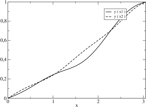
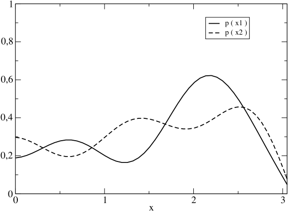
Figure 1: Evaluation of $y$ and $p$ by one iteration of the SFPL algorithm for the Michalewicz’s function, using $L=5$ and $D=1$. Despite the very low number of gradient evaluations used, the algorithm is capable to find a probability structure that is consistent with the global properties of the cost function.

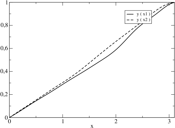
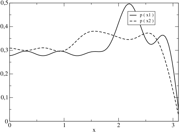
Figure 2: The same case reported in Fig. (1), but using $L=10$.

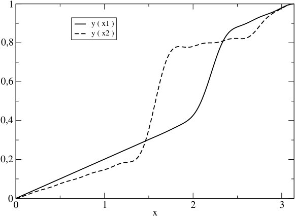
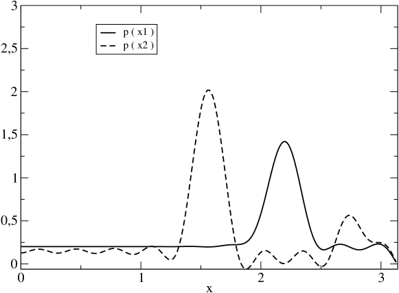
Figure 3: Evaluation of $y$ and $p$ by one iteration of the SFPL algorithm for the Michalewicz’s function. In this case $L=20$ and $D=0.4$. With the increment in precision and the reduction of the randomness parameter, SFPL finds a probability density that is sharply peaked around the global minimum. Notice that the computational effort is still small, involving only $19$ evaluations of the gradient.

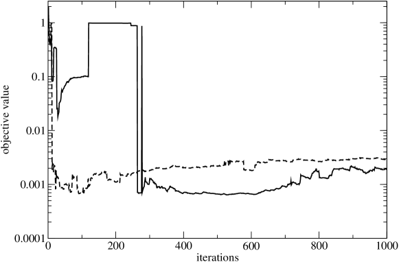
Figure 4: Objective value of the point in which the marginals of the estimated density are maximum for two independent trajectories.

In order to check statistical convergence, the following measures are introduced,

$$av=\frac{1}{N}\sum_{n=1}^{N}\left<x_{n}\right>,$$ (12)

$$s=\frac{1}{N}\sum_{n=1}^{N}\sqrt{\left<x_{n}^{2}\right>-\left<x_{n}\right>^{2}},$$

where the brackets in this case represent statistical moments of the estimated marginals. Under the expansion (9), all the necessary integrals are easily performed analytically.

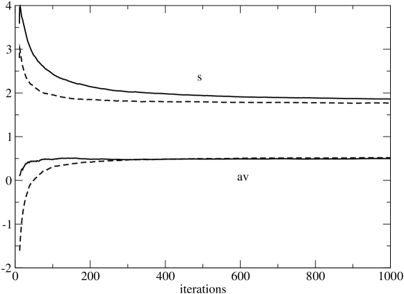
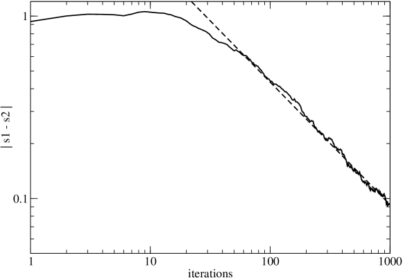
Figure 5: Statistical convergence of the stationary density estimation procedure on the XOR problem. The value of the average first moment and standard deviation of the estimated marginals from two independent trajectories is plotted in the left. The graph on the right shows the distance between both average standard deviations. This distance decay at a geometric rate over the first $\sim 100$ iterations. Asymptotically the distance behave like a power law characterized by $|s_{1}-s_{2}|\sim M^{-0.67}$, where $M$ is the number of iterations.

In the first graph of Fig. 5, the evolution over iterations of the SFP sampler of $s$ and $av$ for two arbitrary and independent trajectories is plotted. A very fast convergence in the measure $av$ is evident. The measure $s$ is further studied in the second graph of Fig. 5, where the difference on that measure among the two trajectories is followed over iterations. The convergence is consistent with a geometric behavior over the first ($\sim 100$) iterations and shows an asymptotic power law rate.

4 Maximum Likelihood Estimation and Bayesian Inference

Besides its applicability like a diversification strategy for local search algorithms, the fast convergence of the SFPL could be fruitful to give efficient aproaches to inference, for instance in the training of neural networks. From the point of view of statistical inference, the uncertainty about unknown parameters of a learning machine is characterized by a posterior density for the parameters given the observed data [16, 14]. The prediction of new data is then performed either by the maximization of this posterior (maximum likelihood estimation) or by an ensemble average over the posterior distribution (Bayesian inference). To be specific, suposse a system which generates an output $Y$ given an input $X$, such that the data is described by a distribution with first moment $E[Y(X)]=f(X,w)$ and diagonal covariance matrix $\sigma^{2}I$. The problem is to estimate $f$ from a given set of observations $S$. The parameters could be, for instance, different neural network weights and architectures. The observed data defines an evidence for the different ensemble members, given by the posterior $p(w|S)$. In maximum likelihood estimation, training consists on finding a single set of optimal parameters that maximize $p(w|S)$. Bayesian inference, on the other hand, is based on the fact that the estimator of $f$ that minimizes the expected squared error under the posterior is given by [16]

$$\hat{Y}=\left<f(X)\right>=\int dwf(X,w)P(w|S),$$ (13)

so training is done by estimating this ensemble average.

In the SFPL framework proposed here, priors are always given by uniform densities. This choice involves very few prior assumptions, regarding the assignment of reasonable intervals on which the components of $w$ lie. Under an uniform prior, and if the data present in the sample has been independently drawn, it turns out that the posterior is given by

$$p(w|S)\propto exp(-V/D)$$ (14)

where $D=2\sigma^{2}$ and $V$ is the given loss function. The SFPL algorithm can be therefore directly applied in order to learn the marginals $p(w_{n}|S)$ of the posterior (14). By construction, these marginals will be properly normalized.

It is now argued that SFPL can be used to efficiently perform maximum likelihood and Bayesian training. Consider again the XOR example. The associated density has been estimated assuming a prior density for each parameter $w_{n}$ over the interval $[-10,10]$. The posterior density, on the other hand, is a consequence of the cost function given the set of training data. In Section 3 it has been shown that for nonseparable nonlinear cost functions like in the XOR case, SFPL converges to a correct estimation of the marginal densities $p(w_{n})$. Therefore, the maximization of the likelihood is reduced to $N$ line maximizations, where $N$ is the number of weights to be estimated. The advantage of this procedure in comparision with the direct maximization of $p(w|S)$ is evident. On the other hand, the SFP sampler itself is designed as a generator of deviates that are drawn from the stationary density. The average (13) can be approximated by

$$\hat{Y}=\left<f(X)\right>\approx\sum_{t}f(X,w^{(t)}),$$ (15)

without the need of direct simulations of the stochastic search, which is necessary in most of other techniques [16].

In Fig. 6 is shown the behavior of $p(w_{n})$ for a particular weight as the sample size increases. The parameters $L=200$ and $D=0.01$ are fixed. The two dotted lines correspond to cases with sample sizes of one and two, with inputs ${(0,0)}$ and ${(0,0),(1,1)}$ respectively. The resulting densities are almost flat in both situations. The dashed line corresponds to a sample size of three. The sample points are ${(0,0),(1,1),(0,1)}$. In this case the sample is large enough to give a sufficient evidence to favor a particular region of the parameter domain. The solid line corresponds to the situation in which all the four points of the data set are used for training. The resulting density is the sharpest. The parameter $D$ is proportional to the noise strength in the stochastic search. It can be selected on the basis of a desired computational effort, as discussed in [3]. Figure 6 indicates that at a fixed noise level $D$, an increase of evidence imply a decrease on the uncertainty of the weights. This finding agrees with what is expected from the known theory of the statistical mechanics of neural networks [15], according to which the weight fluctuations decay as the data sample grows.

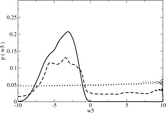
Figure 6: The probability density of a particular weight ($w_{5}$, a bias of one of the neurons in the hidden layer) of the ANN model for the XOR problem. The dotted lines correspond to cases with sample sizes of one and two. The dashed line is for the density that results from a sample of size three while the case for a sample size of four is given by the solid line.

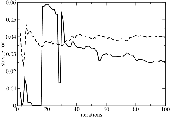
Figure 7: Performance of maximum likelihood (solid) and Bayesian (dashed) training for the XOR problem, using stationary Fokker–Planck learning to estimate weight distributions.

The performance of maximum likelihood and Bayesian training is reported in Fig. 7, using the complete sample for the inference of the weights. The standard deviation of the error of the networks instantiated at the inferred weigths is reported at each iteration. The solid line corresponds to maximum likelihood training, which is essentially the same calculation already reported on Fig. 4. The performance is very similar for Bayesian training, which corresponds to the dashed line. The estimation of the average (15) as been performed by evaluating the neural network on a weight vector drawn by the SFP sampler at each iteration. In this way, the number of terms in the sum of Eq. (15) is equal to the number of iterations of the SFP sampler.

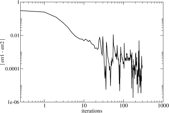
Figure 8: The difference in average cost function value for two independent trajectories in the robot arm problem. The ANN as been trained using $200$ sample points.

A larger example involving noisy data is now presented. Consider the “robot arm problem”, a benchmark that has already been used in the context of Bayesian inference [16]. The data set is generated by the following dynamical model for a robot arm

$$y_{1}=2.0cos(x_{1})+1.3cos(x_{1}+x_{2})+e_{1}$$ (16)

$$y_{2}=2.0sin(x_{1})+1.3sin(x_{1}+x_{2})+e_{2}$$

The inputs $x_{1}$ and $x_{2}$ represent joint angles while the outputs $y_{1}$ and $y_{2}$ give the resulting arm positions. Following the experimental setup proposed in [16], the inputs are uniformly distributed in the intervals $x_{1}\in[-1.932,-0.453]\cup[0.453,1.932]$, $x_{2}\in[0.534,3.142]$. The noise terms $e_{1}$ and $e_{2}$ are Gaussian and white with standard deviation of $0.1$. A sample of $200$ points is generated using these prescriptions. A neural network with one hidden layer consisting on $16$ hyperbolic tangent activation functions is trained on the generated sample using SFP learning, considering a squared error loss function. The same priors are assigned to all of the weights: uniform distributions in the interval $[-1,1]$. The average absolute difference in training errors for two independent trajectories is shown on Fig. 8 for a case in which $L=300$, $D=0.00125$ and $M=300$ iterations. Taking into account that the expected equilibrium square error is $err\approx D/2$, it turns out that the differences between both trajectories are of the same order of magnitude as the expected equilibrium error in about $10$ iterations. During the course of the total of $300$ iterations of SFP of one of the trajectories, the network as been evaluated in the test input $(-1.471,0.752)$. The resulting Bayesian prediction is shown on Fig. 9 in the form of a pair of histograms. The output that would be given by the exact model (16) in the absence of noise is $(1.177,-2.847)$. The Bayesian prediction given by SFPL has its mean at $(1.24,-2.64)$ with a standard deviation of $\approx 0.12$ for each variable. Therefore the output given by the underlying model is contained in the $95\%$ confidence interval around the Bayes expectation. Consistent predictions can also be obtained under less precision and data. In Fig. 10 are shown the histograms obtained for a case with a sample size of $50$ points, $L=200$ and $D=0.01$. Altough the Bayes prediction is more uncertain, it still is statistically consistent with the underlying process.

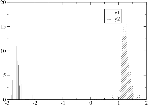
Figure 9: Bayesian predictions for the robot arm problem in the test input $(-1.471,0.752)$. The SFPL parameters are $L=300$, $D=0.00125$ and $M=300$, using $200$ sample points.

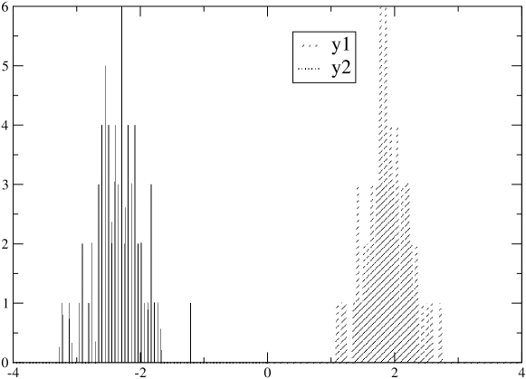
Figure 10: Same case as in Fig. 9 but with SFPL parameters given by $L=200$, $D=0.01$, $M=300$ and sample size of $50$ points.

In the robot arm example the number of gradient evaluations needed to approximately converge to the equilibrium density in the $L=300$ case was about $2(L-1)M\sim 5980$. This seems competitive with respect to previous approaches, like the hybrid Monte Carlo strategy introduced by Neal. The reader is referred to Neal’s book [16] in order to find a very detailed application of hybrid Monte Carlo to the robot arm problem. An additional advantage of the SFPL method lies on the fact that explicit expressions for the parameter’s densities are obtained.

Much more detailed experimentation is under current development. Additional studies regarding issues like generalization of more complex ANN models under a limited amount of data, in the spirit of the general framework for Bayesian learning [16, 14], is currently a work in progress by the author.

5 Conclusion

Theoretical and empirical evidence for the characterization of the convergence of the density estimation of stochastic search processes by the method of stationary Fokker–Planck learning as been presented. In the context of nonlinear optimization problems, the procedure turns out to converge in one iteration for separable problems and displays fast convergence for nonseparable cost functions. The possible applications of stationary Fokker–Planck learning in the development of efficient and reliable maximum likelihood and Bayesian ANN training techniques have been outlined.

References

- [1] K. P. Bennett, E. Parrado-Hernández, The Interplay of Optimization and Machine Learning Research, Journal of Machine Learning Research 7 (2006) 1265–1281.
- [2] A. Berrones, Generating Random Deviates Consistent with the Long Term Behavior of Stochastic Search Processes in Global Optimization, in: Proc. IWANN 2007, Lecture Notes in Computer Science, Vol. 4507 (Springer, Berlin, 2007) 1-8.
- [3] A. Berrones, Stationary probability density of stochastic search processes in global optimization, J. Stat. Mech. (2008) P01013.
- [4] A. Canty, Hypothesis Tests of Convergence in Markov Chain Monte Carlo, Journal of Computational and Graphical Statistics 8 (1999) 93-108.
- [5] R. Chelouah, P. Siarry, Tabu Search Applied to Global Optimization. European Journal of Operational Research 123 (2000) 256-270.
- [6] L. Devroye, Non-Uniform Random Variate Generation (Springer, Berlin, 1986).
- [7] A. E. Eiben, J. E. Smith, Introduction to Evolutionary Computing, (Springer, Berlin, 2003).
- [8] S. Geman, D. Geman, Stochastic relaxation, Gibbs distributions, and the Bayesian restoration of images, IEEE Trans. Pattern Anal. Machine Intell. 6 (1984) 721-741.
- [9] S. Geman, C. R. Hwang, Diffusions for Global Optimization SIAM J. Control Optim. 24 5 (1986) 1031-1043.
- [10] D. Goldberg, Genetic Algorithms in Search, Optimization and Machine Learning, (Addison–Wesley, 1989).
- [11] A. Hertz, D. Kobler, A framework for the description of evolutionary algorithms, European Journal of Operational Research 126 (2000) 1-12.
- [12] http://www.informs.org/
- [13] S. Kirkpatrick, C. D. Gelatt Jr., M. P. Vecchi, Optimization by Simulated Annealing, Science 220 (1983) 671-680.
- [14] D. J. C. MacKay, A practical Bayesian framework for backpropagation networks, Neural Computation 4 3 (1992) 448 - 472.
- [15] D. Malzahn, M. Opper, Statistical Mechanics of Learning: A Variational Approach for Real Data, Phys. Rev. Lett. 89 10 (2002) 108302.
- [16] R. M. Neal, Bayesian Learning for Neural Networks, (Springer, Berlin, 1996).
- [17] H. Risken, The Fokker–Planck Equation, (Springer, Berlin, 1984).
- [18] G. O. Roberts, N. G. Polson, On the Geometric Convergence of the Gibbs Sampler J. R. Statist. Soc. B 56 2 (1994) 377-384.
- [19] P. Y. Papalambros, D. J. Wilde, Principles of Optimal Design: Modeling and Computation, (Cambridge University Press, 2000).
- [20] P. Parpas, B. Rustem, E. N. Pistikopoulos, Linearly Constrained Global Optimization and Stochastic Differential Equations Journal of Global Optimization 36 2 (2006) 191-217.
- [21] K. E. Parsopoulos, M. N. Vrahatis, Recent approaches to global optimization problems through Particle Swarm Optimization, Natural Computing 1 (2002) 235-306.
- [22] M. Pelikan, D. E. Goldberg, F. G. Lobo, A Survey of Optimization by Building and Using Probabilistic Models, Computational Optimization and Applications 21 1 (2002) 5-20.
- [23] D. Peña, R. Sánchez, A. Berrones, Stationary Fokker–Planck Learning for the Optimization of Parameters in Nonlinear Models, in: Proc. MICAI 2007, Lecture Notes in Computer Science Vol. 4827, (Springer, Berlin, 2007) 94-104.
- [24] W. Press, S. Teukolsky, W. Vetterling, B. Flannery, Numerical Recipes in C++, the Art of Scientific Computing, (Cambridge University Press, 2005).
- [25] J. A. K. Suykens, H. Verrelst, J. Vandewalle, On–Line Learning Fokker–Planck Machine. Neural Processing Letters 7 2 (1998) 81-89.
- [26] N. G. Van Kampen, Stochastic Processes in Physics and Chemistry, (North-Holland, 1992).