Orbits and Masses in the T Tauri System

Abstract

Aims. We investigate the binary star T Tauri South, presenting the orbital parameters of the two components and their individual masses.

Methods. We combined astrometric positions from the literature with previously unpublished VLT observations. Model fits yield the orbital elements of T Tau Sa and Sb. We use T Tau N as an astrometric reference to derive an estimate for the mass ratio of Sa and Sb.

Results. Although most of the orbital parameters are not well constrained, it is unlikely that T Tau Sb is on a highly elliptical orbit or escaping from the system. The total mass of T Tau S is rather well constrained to $3.0^{+0.15}_{-0.24}\rm\,M_{\odot}$. The mass ratio Sb:Sa is about 0.4, corresponding to individual masses of $M_{\rm Sa}=2.1\pm 0.2\,M_{\odot}$ and $M_{\rm Sb}=0.8\pm 0.1\,M_{\odot}$. This confirms that the infrared companion in the T Tauri system is a pair of young stars obscured by circumstellar material.

1 Introduction

T Tauri was discovered in 1852 by Hind during observations of the bright variable nebula NGC 1555 (Hind’s nebula) (Bertout 1984). Almost a century later, Joy (1945) defined a new class of variables, which contained eleven stars initially. The members of the class were later identified as low-mass pre-main-sequence objects. Joy named these sources ‘T Tauri variables’, because T Tau not only shows the typical features, but also is among the brightest and best known objects of this group.

However, as observational techniques improved, the character of T Tau turned out to be more peculiar than prototypical. One of the most surprising findings was made by Dyck et al. (1982). They observed T Tau using one-dimensional speckle interferometry and found an infrared companion with a separation of less than one arcsecond. However, neither the relative position of the two sources nor the identification of the visually bright component could be derived. Radio observations (Cohen et al. 1982) and subsequent astrometric comparisons between the radio and the optical data revealed that the infrared companion was located $0\aas@@fstack{\prime\prime}7\pm 0\aas@@fstack{\prime\prime}1$ (de Vegt 1982) or $0\aas@@fstack{\prime\prime}6\pm 0\aas@@fstack{\prime\prime}1$ (Hanson et al. 1983) south of the visually bright component. The southern component dominates the system longward of the near-infared wavelength regime, but no optical counterpart could be identified down to 19.6 mag in the V-band (Stapelfeldt et al. 1998).

Explanations of the physical nature of the enigmatic infrared companion ranged from a true protostar still embedded in its contracting envelope (Bertout 1983), to a FUOr-like source with the observed rapid brightening due to accretion (Ghez et al. 1991), to a normal T Tauri star coeval with its primary. In the latter case, the star has to be obscured either due to a special viewing geometry through the circumstellar material (Calvet et al. 1994) or enhanced accretion (Koresko et al. 1997).

Considerable observational and theoretical effort has been expanded to understand this source. Perhaps the most important ingredient in solving this puzzle came surprisingly: the resolution of the southern companion into two sources using speckle holography (Koresko 2000). With a separation of ${}\sim 0\aas@@fstack{\prime\prime}05$, the two components were named T Tau Sa and T Tau Sb. T Tau Sb has been identified as a heavily extincted, actively accreting pre-main-sequence star with a spectral type M1 (Duchêne et al. 2002), while the spectrum of T Tau Sa is featureless except for a strong Br$\gamma$ emission line, leaving the nature of the object uncertain.

The northern of the two radio sources found by Schwartz et al. (1984) is easy to identify with T Tau N, but it was not clear which of the two components of T Tau S should be identified with the southern radio source. Johnston et al. (2003) and Loinard et al. (2003, 2005) associated the radio source with T Tau Sb. This would require that the orbital motion of T Tau Sb around T Tau Sa shows a dramatic change between 1995 and 1998, probably caused by the ejection of Sb from the T Tau S system (Loinard et al. 2003). However, Furlan et al. (2003) found that T Tau Sb and the radio source have distinct paths, and suggested a fourth object as the source of the southern radio emission. After further refinement of the picture, it has been concluded that the radio source may be connected with, but not identical to the infrared source (Johnston et al. 2004a, b; Loinard et al. 2007a).

For completeness, we note that the detection of another source $0\aas@@fstack{\prime\prime}27$ north of T Tau N has been reported by Nisenson et al. (1985). They identified a second component in the visual wavelength regime, which was later detected in the K-band by Maihara & Kataza (1991). However, this source was not detected by Gorham et al. (1992) nor by Stapelfeldt et al. (1998). If the additional source exists, probable explanations for the non-detections are that the source is variable either intrinsically or due to varying extinction. The latter is not unlikely considering the complex environment of T Tau (Solf & Böhm 1999; Herbst et al. 2007).

The presence of the companion Sb at such a small separation offers the possibility to trace the orbital motion of T Tau Sa and Sb around each other in a reasonable time and with no influence of T Tau N in first order approximation. This can lead to the determination of the dynamical mass of T Tau S and – with the help of the common orbit of the southern pair around the northern component – the individual masses of T Tau Sa and Sb. Such information is essential to judge the different models. In addition, evolutionary models of pre-main-sequence objects may benefit from the direct measurement of stellar masses, since only a few young stellar objects have masses known independent of theoretical assumptions.

Duchêne et al. (2006) made such a dynamical analysis of the T Tau S system using measurements in both the near-infrared and radio. A simultaneous fit of the Keplerian orbit of T Tau Sb around T Tau Sa and the orbital motion of T Tau Sb around T Tau N lead to a dynamical mass of $3.34\pm 0.36\,\rm{M}_{\odot}$ for the southern binary and a mass ratio Sb:Sa of $0.18\pm 0.04$. This result is consistent with earlier determinations of the individual masses (Johnston et al. 2004a, b). The improved accuracy allows us to conclude that T Tau Sa with $2.73\pm 0.31\,\rm{M}_{\odot}$ may be a Herbig Ae star whose light is extincted by a highly inclined circumstellar disc (Kasper et al. 2002; Duchêne et al. 2005, 2006). The derived mass of T Tau Sb is $0.61\pm 0.17\,\rm{M}_{\odot}$, in good agreement with its early M-type spectrum. Duchêne et al. (2006) modeled the orbital motion of T Tau S around N by polynomials in $x$ and $y$. This does not allow a determination of the system mass, and prevents the derivation of the dynamical mass of T Tau N.

In this paper, we further refine our knowledge of the orbits and thus of the individual masses. We restrict ourselves to measurements made in the near-infrared, since the identification of the radio sources with T Tau Sb is uncertain (Loinard et al. 2007b). A further complication comes from the fact that T Tau Sa has not been detected in radio observations. The position of Sb relative to Sa can only be computed indirectly, using the position of T Tau N and the estimated parameters of the orbits.

We also explore the confidence limits for the resulting orbital elements, a crucial step when interpreting such highly degenerate orbits as those in the T Tau triple system.

The data from the literature, as well as the reduction and analysis of our own measurements, are presented in Section 2. In Section 3, the fit of the orbital elements and the determination of the mass ratio is explained. The reliability of the fit and its implications for our current knowledge of the T Tau system is discussed in Section 4. In Section 5 we summarize our results.

2 Observations

2.1 Literature

T Tauri has been observed in the near-infrared with various telescopes and instruments since the discovery of its binary nature. Most of the measurements used in this work thus were taken from the literature (see Tables 1 and 2). The tables include all statistical and systematic errors reported by the authors in the papers or in follow-up studies. The data of the observations that did not resolve the southern binary are listed in Table 1. Table 2 lists observations that did resolve T Tau S and gives the positions of component Sa relative to N and Sb, respectively. Duchêne et al. (2006) give only positions of Sb relative to N and Sa; the position of Sa relative to N has been computed by us, taking the propagation of errors into account.

Table 1: Astrometric Measurements of T Tau N – S (S unresolved)

Date (UT)	$d$ [mas]		P.A. $[^{\circ}]$		Source
1989 Dec 10	$720$ ${}\pm{}$	$14$	$175.5$ ${}\pm{}$	$1.0$	Ghez et al. (1995)
1990 Nov 10	$716$ ${}\pm{}$	$14$	$176.2$ ${}\pm{}$	$1.0$	Ghez et al. (1995)
1991 Nov 19	$702$ ${}\pm{}$	$14$	$176.4$ ${}\pm{}$	$1.0$	Ghez et al. (1995)
1992 Feb 20	$710$ ${}\pm{}$	$14$	$176.7$ ${}\pm{}$	$1.0$	Ghez et al. (1995)
1992 Oct 11	$692$ ${}\pm{}$	$15$	$177.0$ ${}\pm{}$	$1.4$	Ghez et al. (1995)
1993 Nov 25	$701$ ${}\pm{}$	$14$	$177.0$ ${}\pm{}$	$1.0$	Ghez et al. (1995)
1993 Dec 26	$690$ ${}\pm{}$	$14$	$176.0$ ${}\pm{}$	$1.1$	Ghez et al. (1995)
1994 Sep 22	$689$ ${}\pm{}$	$14$	$175.9$ ${}\pm{}$	$1.2$	Ghez et al. (1995)
1994 Oct 19	$689$ ${}\pm{}$	$14$	$178.2$ ${}\pm{}$	$1.1$	Ghez et al. (1995)
1994 Dec 25	$718$ ${}\pm{}$	$9$	$177.6$ ${}\pm{}$	$0.7$	Roddier et al. (2000)
1997 Nov 17	$709$ ${}\pm{}$	$6$	$180.2$ ${}\pm{}$	$0.5$	Roddier et al. (2000)
1998 Nov  2	$704$ ${}\pm{}$	$6$	$180.7$ ${}\pm{}$	$0.5$	Roddier et al. (2000)
1999 Nov 23	$699$ ${}\pm{}$	$6$	$181.0$ ${}\pm{}$	$0.5$	Roddier et al. (2000)
1997 Dec  4	$685$ ${}\pm{}$	$13$	$179.5$ ${}\pm{}$	$1.0$	White & Ghez (2001)
1997 Dec  6	$698$ ${}\pm{}$	$13$	$179.1$ ${}\pm{}$	$1.0$	White & Ghez (2001)
2000 Feb 20	$691$ ${}\pm{}$	$2$	$181.7$ ${}\pm{}$	$0.8$	This work

Table 2: Astrometric Measurements of T Tau N – Sa – Sb

Date (UT)

T Tau N - Sa

T Tau Sa - Sb

Source

$d$ [mas]

P.A. $[^{\circ}]$

$d$ [mas]

P.A. $[^{\circ}]$

1997 Oct 12

$693$ ${}\pm{}$

$12$

$178.6$ ${}\pm{}$

$0.9$

$\phantom{1}51$ ${}\pm{}$

$9$

$218$ ${}\pm{}$

$8$

Duchêne et al. (2006)

1997 Dec 15

–

–

$\phantom{1}53$ ${}\pm{}$

$9$

$225$ ${}\pm{}$

$8$

Koresko (2000)

2000 Feb 20

$686.3$ ${}\pm{}$

$2.4$

$180.5$ ${}\pm{}$

$0.8$

$\phantom{1}79$ ${}\pm{}$

$2$

$253$ ${}\pm{}$

$2$

This work / Köhler et al. (2000a)

2000 Nov 19

$702$ ${}\pm{}$

$5$

$180.8$ ${}\pm{}$

$0.2^{\mathrm{a}}$

$\phantom{1}92$ ${}\pm{}$

$3$

$268.1$ ${}\pm{}$

$1.6^{\mathrm{a}}$

Duchêne et al. (2002)

2002 Oct 30

$697.6$ ${}\pm{}$

$2.1$

$183.3$ ${}\pm{}$

$0.3$

$106.5$ ${}\pm{}$

$2.6$

$284.5$ ${}\pm{}$

$1.4$

Schaefer et al. (2006)b

2002 Nov 20

$693$ ${}\pm{}$

$4$

$183$ ${}\pm{}$

$1$

$\phantom{1}94.3$ ${}\pm{}$

$3.3$

$278$ ${}\pm{}$

$1$

Mayama et al. (2006)

2002 Dec 13

$695$ ${}\pm{}$

$7$

$183.3$ ${}\pm{}$

$0.7$

$108$ ${}\pm{}$

$1$

$284.9$ ${}\pm{}$

$0.9$

Duchêne et al. (2005)

2002 Dec 15

$693.5$ ${}\pm{}$

$1.4$

$182.3$ ${}\pm{}$

$0.3$

$106.4$ ${}\pm{}$

$1.6$

$283.9$ ${}\pm{}$

$0.4$

This work

2002 Dec 20

–

–

$110$ ${}\pm{}$

$4$

$282$ ${}\pm{}$

$2.1$

Beck et al. (2004)

2002 Dec 24

$691$ ${}\pm{}$

$12$

$181.7$ ${}\pm{}$

$1.1$

$108$ ${}\pm{}$

$5$

$287.8$ ${}\pm{}$

$2.6$

Furlan et al. (2003)

2003 Nov 18

$700.4$ ${}\pm{}$

$2.9$

$183.2$ ${}\pm{}$

$0.6$

$116.5$ ${}\pm{}$

$3.1$

$291$ ${}\pm{}$

$1.6$

Schaefer et al. (2006)

2003 Dec 12

$698$ ${}\pm{}$

$5$

$181.9$ ${}\pm{}$

$1.2$

$118$ ${}\pm{}$

$2$

$288.6$ ${}\pm{}$

$1.1$

Duchêne et al. (2005)

2003 Dec 12

$696.2$ ${}\pm{}$

$2.0$

$182.8$ ${}\pm{}$

$0.1$

$113.3$ ${}\pm{}$

$1.0$

$288.5$ ${}\pm{}$

$0.8$

This work

2004 Nov 23

$690$ ${}\pm{}$

$3$

$186$ ${}\pm{}$

$1$

$100$ ${}\pm{}$

$2$

$298$ ${}\pm{}$

$1$

Mayama et al. (2006)

2004 Dec  9

$693.2$ ${}\pm{}$

$1.2$

$183.5$ ${}\pm{}$

$0.1$

$118.9$ ${}\pm{}$

$1.1$

$295.9$ ${}\pm{}$

$0.6$

This work

2004 Dec 19

$689$ ${}\pm{}$

$3$

$183.6$ ${}\pm{}$

$0.4$

$116$ ${}\pm{}$

$4$

$294.1$ ${}\pm{}$

$1.4$

Duchêne et al. (2006)

2004 Dec 24

$698.5$ ${}\pm{}$

$2.2$

$184.7$ ${}\pm{}$

$0.3$

$119.6$ ${}\pm{}$

$2.8$

$297.2$ ${}\pm{}$

$1.4$

Schaefer et al. (2006)

2005 Feb  9

$704.0$ ${}\pm{}$

$1.6$

$184.4$ ${}\pm{}$

$0.1$

$120.7$ ${}\pm{}$

$1.9$

$300.4$ ${}\pm{}$

$0.9$

Schaefer et al. (2006)

2005 Mar  9

$702.8$ ${}\pm{}$

$2.4$

$184.4$ ${}\pm{}$

$0.2$

$120.3$ ${}\pm{}$

$2.9$

$300.6$ ${}\pm{}$

$1.4$

Schaefer et al. (2006)

2005 Mar 24

$703.7$ ${}\pm{}$

$0.9$

$184.3$ ${}\pm{}$

$0.1$

$121.5$ ${}\pm{}$

$1.2$

$300.4$ ${}\pm{}$

$0.6$

Schaefer et al. (2006)

2005 Oct 20

$703.3$ ${}\pm{}$

$1.2$

$184.9$ ${}\pm{}$

$0.1^{\mathrm{c}}$

$123.7$ ${}\pm{}$

$1.3$

$303.3$ ${}\pm{}$

$0.6$

Schaefer et al. (2006)

2005 Nov 13

$694$ ${}\pm{}$

$2$

$184.4$ ${}\pm{}$

$0.2$

$119$ ${}\pm{}$

$1$

$300.6$ ${}\pm{}$

$1.0$

Duchêne et al. (2006)

2005 Dec  6

$703.0$ ${}\pm{}$

$5.7$

$185.8$ ${}\pm{}$

$0.5$

$121.9$ ${}\pm{}$

$6.8$

$304.8$ ${}\pm{}$

$3.2$

Schaefer et al. (2006)

2006 Oct 11

$694.4$ ${}\pm{}$

$0.9$

$184.9$ ${}\pm{}$

$1.0$

$125.1$ ${}\pm{}$

$0.7$

$304.7$ ${}\pm{}$

$1.0$

This work

2007 Sep 16

$693.6$ ${}\pm{}$

$1.8$

$185.0$ ${}\pm{}$

$0.2$

$127.0$ ${}\pm{}$

$0.5$

$308.2$ ${}\pm{}$

$0.3$

This work

• Corrected value according to Duchêne et al. (2006)

• This is a re-analysis of the data presented in Beck et al. (2004) using a more sophisticated PSF fitting routine.

• $90^{\circ}$ subtracted from the position angle in Schaefer et al. (2006) to correct for the orientation of the camera (Schaefer, priv. comm.).

2.2 ALFA

Köhler et al. (2000a) presented results of observations obtained in February 2000 with the adaptive optics system ALFA at the 3.5 m telescope on Calar Alto, Spain. The $H$ photometric band was used to take advantage of the smaller diffraction limit compared to the $K$ band. T Tau N served as PSF-reference to deconvolve T Tau S using speckle interferometric techniques. This allowed them to resolve the Sa-Sb binary, and confirm the discovery of Koresko (2000).

We revisited these observational data, in order to measure the position of component Sa relative to N. In our new analysis, we used observations of the star PPM 119798, taken shortly after the images of T Tauri, to deconvolve the triple system. We again applied our own speckle program; for a detailed description see, e.g., Köhler et al. (2000b). The resulting visibility appears in Fig. 1. It clearly shows the characteristic fringe pattern of the N-S binary. However, the signal of the Sa-Sb pair is obscured by random fluctuations. One has to keep in mind that T Tau N contributes more than 90 % of the flux of the system in the $H$ band, resulting in correspondingly high speckle noise. Therefore, it was not possible to measure the relative position of T Tau N and Sa, but only the position of the combined light of Sa and Sb relative to N. The latter is listed in Table 1. We then computed the offset of T Tau Sa from the center of light of Sa and Sb, using the known position of Sa relative to Sb and the flux ratio of Sb/Sa of $0.259\pm 0.011$ (Köhler et al. 2000a). The results are given in Table 2.

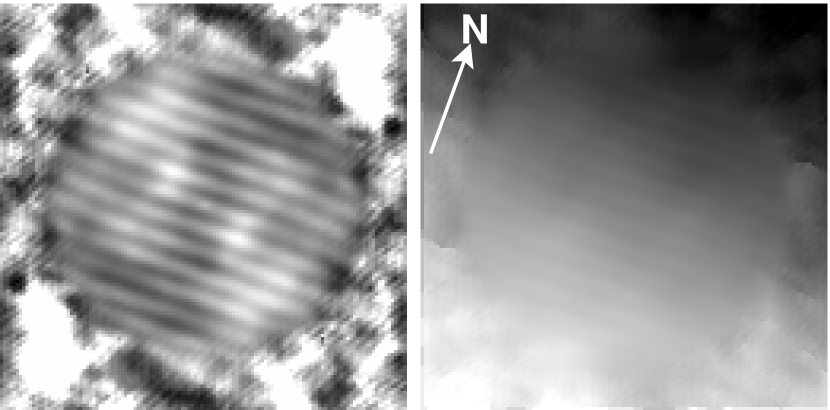
Figure 1: Result of the speckle-observation of T Tauri on February 20, 2000. Shown are modulus (left) and phase (right) of the complex visibility (the Fourier-transform of the image). The N-S binary pair causes the fringe pattern in the modulus and the steps in the phase. The fringe pattern due to the binary nature of T Tau S is too weak to be recognizable.

2.3 NAOS/CONICA

We also report on observations with NAOS/CONICA (NACO for short), the adaptive optics, near-infrared camera at the ESO Very Large Telescope on Cerro Paranal, Chile (Rousset et al. 2003; Lenzen et al. 2003). They are marked “this work” in Table 2. The NACO observations in 2002 and 2003 were carried out in the course of the NACO Guaranteed Time Observations (PI Tom Herbst), while the observations in 2004, 2006, and 2007 were regular proposals for open time. We use only imaging observations in the $K$ or $K_{s}$ photometric band for the orbit determination.

The NACO images were sky subtracted with a median sky image, and bad pixels were replaced by the median of the closest good neighbors. Finally, the images were visually inspected for any artifacts or residuals. Figure 2 shows an example of the results.

The Starfinder program (Diolaiti et al. 2000) was used to measure the positions of the stars. The positions in several images taken during one observation were averaged, and their standard deviation used to estimate the errors. To derive the exact pixel scale and orientation of the detector, we took images of fields in the Orion Trapezium during each observing campaign. The measured positions of the stars were compared with the coordinates given in McCaughrean & Stauffer (1994) by the astrometric software ASTROM. The calibrated separations and position angles appear in Table 2.

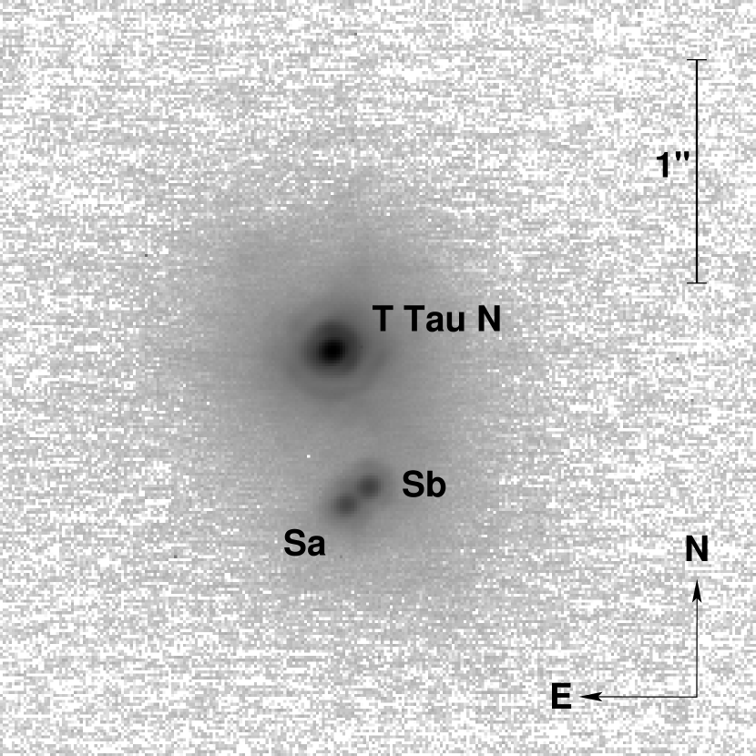
Figure 2: Image of the T Tau system taken with NACO in the $K_{s}$ photometric band on 2006 Oct 11, shown with a logarithmic scale.

3 Orbit Determination

3.1 The Orbit of T Tauri Sa/Sb

We estimated the orbital parameters of the Sa-Sb pair by fitting orbit models to all observations listed in Table 2, except the positions given by Mayama et al. (2006). These two data points show significant offsets from all the other measurements (Fig. 6 and 7). Since we do not know the reason for this discrepancy and have no way to correct it, we excluded these points from the fit. To avoid any systematic errors due to uncertainties of the distance, the separations are expressed in units of milli-arcseconds within the fitting program. Only the final result was converted to AU.

To find the orbital fit with the minimum $\chi^{2}$, we employed a method similar to that outlined in Hilditch (2001): a grid-search in eccentricity $e$, period $P$, and time of periastron $T_{0}$. At each grid point, the Thiele-Innes elements were determined by a linear fit to the observational data using Singular Value Decomposition. From the Thiele-Innes elements, the semimajor axis $a$, the angle between node and periastron $\omega$, the position angle of the line of nodes $\Omega$, and the inclination $i$ were computed.

We decided to scan a wide range of parameter values: 200 points within $0\leq e\leq 2$, 250 points within $10{\rm\,yr}\leq P<3100{\rm\,yr}$, and initially 100 points for $T_{0}$ distributed over one orbital period. After the initial scan over $T_{0}$, the best estimate for $T_{0}$ was improved by re-scanning a narrower range in $T_{0}$ centered on the minimum found in the coarser scan. The range was reduced by a factor of 10, but the number of grid points was held constant. This grid refinement was repeated until the step size was less than one day.

For every point in the $e$-$P$-plane, the set of orbital elements resulting in the minimum $\chi^{2}$ was stored, to allow later analysis of $\chi^{2}$ as a function of $e$ and $P$. The parameter giving the time of periastron $T_{0}$ is periodic: we obtain the same orbit if we add one orbital period to $T_{0}$. Furthermore, a change in $T_{0}$ only shifts the position at a given time within the orbit. A value of $T_{0}$ that has a small offset from the optimal $T_{0}$ will therefore shift the expected positions away from the measured positions and result in a larger $\chi^{2}$. For these reasons, we are confident that our grid search found the globally optimum $T_{0}$ and did not store all the sets of orbital elements for non-optimum $T_{0}$.

The resulting $\chi^{2}$-minimum is very broad (Figs. 3 – 5). For example, Fig. 3 shows that orbits with periods between 30 and more than 1000 years are within $\Delta\chi^{2}<1$ of the best orbit (the $1\sigma$ confidence limit, Press et al. 1992). The situation for the eccentricity $e$ is similar (Fig. 4): Eccentricities between about 0.4 and 0.8, and even some unbound orbits with $e>1$ are within $\Delta\chi^{2}<1$.

Figure 3: The result of the first step in our orbit-fitting procedure. Shown is the minimum $\chi^{2}$ for a given period, i.e. we hold the period fixed and search for the optimum set of the remaining 6 orbital elements. Solutions with unphysically high system masses (${}>250\rm\,M_{\sun}$) have been excluded. The ripples at periods ${}\ga 200$ years are artefacts caused by the grid search. Note that the $\chi^{2}$ shown here has not been divided by the number of degrees of freedom.

Figure 4: Like Fig. 3, but showing the minimum $\chi^{2}$ as function of eccentricity instead of period. Note that some orbits with $e>1$ (i.e. unbound orbits) have a $\chi^{2}$ not much higher than the minimum.

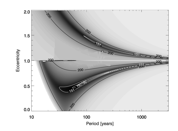
Figure 5: Contour plot of the minimum $\chi^{2}$ as function of period and eccentricity. The contour $\chi^{2}=151$ marks the 68 % confidence intervals for the period or eccentricity (cf. Figs. 3 and 4).

We improved the results of the grid-search with a Levenberg-Marquardt $\chi^{2}$ minimization algorithm (Press et al. 1992) that fits for all 7 parameters simultaneously. The simple-minded approach would be to use the orbital elements with the minimum $\chi^{2}$ found with the grid-search. However, given the structure of the $\chi^{2}$-plane (Fig. 5), there is always the danger that the algorithm converges on a local instead of the global minimum. To avoid this, we decided to use all orbits resulting from the grid-search as starting points and carried out $250\times 200$ runs of the Levenberg-Marquardt algorithm (the grid spans 250 periods and 200 eccentricities). The orbit with the globally minimum $\chi^{2}$ found in this way is shown in Figs. 6 and 7, and its elements are listed in Table 3.

3.1.1 Error estimates for the Orbital Elements

The Levenberg-Marquardt algorithm also computes the covariance matrix of the fitted orbital parameters, which allows derivation of standard error estimates for the parameters. However, the algorithm assumes that the $\chi^{2}$ function can be approximated by a quadratic form in the region close to the minimum. While this is a reasonable assumption for iteratively searching the minimum, it is clearly a rather bad assumption if one is interested in confidence limits for the fitted parameters (cf. Fig. 3 and 4). Better error estimates can be obtained by studying the $\chi^{2}$ function around its minimum (Press et al. 1992). Since we are interested in the confidence interval for each parameter taken separately, we have to perturb one parameter (for example $T_{0}$) away from the minimum, and optimize all the other parameters. Any perturbation of a parameter will of course lead to a larger $\chi^{2}$. The range in $T_{0}$ within which $\chi^{2}(T_{0})-\chi^{2}_{\rm min}<1$ defines the 68 % confidence interval for $T_{0}$. This interval is usually not symmetric around the $T_{0}$ of the best fit, therefore we list in Table 3 separate limits for positive and negative perturbations. It should be noted that these limits describe the parameter range that contain 68 % of the probability distribution, which is equivalent to the commonly used $1\sigma$-errors. However, the errors are not normally distributed, therefore a $2\sigma$ interval will not contain 95 % of the probability distribution.

Table 3: Parameters of the best orbital solution for Sa – Sb.

Orbital Element		Value
Date of periastron $T_{0}$		$2451091$	$\,{}^{+250}_{-1200}$
		(1998 Oct 4)
Period $P$ (years)		$93$	$\,{}^{+115}_{-55}$
Semi-major axis $a$ (mas)		$201$	$\,{}^{+430}_{-110}$
Semi-major axis $a$ (AU)		$30$	$\,{}^{+63}_{-16}$
Eccentricity $e$		$0.57$	$\,{}^{+0.20}_{-0.22}$
Argument of periastron $\omega$ (∘)		$300.6$	$\,{}^{+12.0}_{-30.0}$
P.A. of ascending node $\Omega$ (∘)		$283.2$	$\,{}^{+4.0}_{-7.0}$
Inclination $i$ (∘)		$55.1$	$\,{}^{+2.0}_{-20.0}$
System mass $M_{S}$ ($M_{\odot}$)		$2.96$	$\,{}^{+0.15}_{-0.24}$
reduced $\chi^{2}$		$3.8$
Mass ratio $M_{\rm Sb}/M_{\rm Sa}$		$0.39$	$\,\pm 0.06$
Mass of Sa $M_{\rm Sa}$ ($M_{\odot}$)		$2.13$	$\,{}^{+0.14}_{-0.20}$
Mass of Sb $M_{\rm Sb}$ ($M_{\odot}$)		$0.83$	$\,{}^{+0.10}_{-0.11}$

Orbits with $\chi^{2}-\chi^{2}_{\rm min}<1$ are not necessarily all within a single region in parameter space around the global minimum. There may be local minima that also fulfill the criterion. In fact, some of our Levenberg-Marquardt fits converged on orbital solutions with eccentricity $e>1$ and $\chi^{2}-\chi^{2}_{\rm min}<1$. These orbits are within the 68 % confidence limit. Therefore, we cannot fully exclude that the system is unbound, although it is more likely to be bound.

Figure 6: Best fitting orbit of T Tau Sb around Sa, in the rest frame of Sa. The observed positions are marked by their error ellipses and lines connecting the observed and calculated position at the time of the observations. The dash-dotted line indicates the line of nodes, the dashed line the periastron, and the arrow shows the direction of the orbital motion. The two dash-dotted ellipses are the measurements by Mayama et al. (2006).

Figure 7: Detailed view of the orbit of T Tau Sb in the rest frame of Sa, and the observations since 2002. The symbols are the same as in Fig. 6.

The system mass $M_{S}$ given in Table 3 is computed from the semi-major axis and the period. To convert the angular separation in milli-arcseconds (mas) to a linear separation in AU, a distance to T Tau of $146.7\pm 0.6\rm\,pc$ was adopted (Loinard et al. 2007b). The semi-major axis $a$ and the period $P$ of the T Tau S binary are correlated around the minimum of the $\chi^{2}$-surface: If one sets the period to a value higher than at the minimum $\chi^{2}$ and optimizes the other 6 parameters, then the resulting $a$ will also be larger than at the global minimum. This has to be taken into account in the computation of the error of the system mass. One way to do this is to take into account the covariance of $a$ and $P$. However, since the covariance matrix is a good approximation only in a small region around the $\chi^{2}$ minimum, we choose a different approach: During the determination of the confidence intervals for $a$ and $P$, we also compute the system mass. The maximum and minimum masses within the region where $\Delta\chi^{2}<1$ are adopted as confidence limits and listed in Table 3. It is worth noting that we did not have to decide whether we want to use the results from the confidence interval in $a$ or in $P$ – the orbits are identical. This is caused by the strong correlation between $a$ and $P$, which in turn leads to a small error in $M_{S}$ compared to the larger uncertainties in $a$ and $P$ (see also Sect. 4.2).

3.2 The Orbit of T Tauri S and the Mass Ratio Sb/Sa

The positions of T Tau Sb relative to Sa allow us to determine only the combined mass of Sa and Sb. To compute the individual masses, we need to know the mass ratio $q$, which can be computed if the position of the center of mass (CM) of Sa and Sb is known. Unfortunately, we cannot observe the CM directly. However, we know that the CM of Sa and Sb is in orbit around T Tau N, and that Sa and Sb are in orbit around their CM (see Fig. 8).

Figure 8: Schematic representation of the stars and orbits in the T Tauri system. The origin of the coordinate system is fixed on T Tau N (marked by a plus sign), therefore the center of mass of Sa and Sb describes an orbit around N. The orbit resulting from our model fits is indicated by the dashed line, while the position of the CM of Sa and Sb on February 20, 2000 is denoted by an asterisk. The orbits of Sa and Sb around their CM according to our model fits are drawn as dotted lines, the positions of the stars on February 20, 2000 (computed from the model) are marked by a diamond and a triangle.

One might think that in order to derive the mass ratio $q$, it is necessary to create a model of the entire triple system, and fit both the orbit of the CM, the orbit of Sa and Sb, and the mass ratio simultaneously. However, we know that the CM is always on the line between Sa and Sb, and its distance from Sa is the constant fraction $q/(1+q)$ of the separation of Sa and Sb. The positions of Sa and Sb are usually observed at the same time as N, so we can use the observed separation vectors Sa-Sb instead of a model orbit.

Our model describes the position of the CM of Sa and Sb in two ways: First, it is on a Keplerian orbit around N, which is described by 7 orbital elements. Second, the position of the CM can be computed from the positions of Sa and Sb, and the mass ratio (which is treated as a free parameter). Standard error propagation is used to obtain an error estimate for this position. To compute $\chi^{2}$, we compare the position of the CM from the orbit around N with the positions derived from the observations. Our model has therefore only 8 free parameters, the 7 elements which describe the orbit of the CM of Sa/b around N, and the parameter $f=q/(1+q)$. The parameter $f$ is often called fractional mass (Heintz 1978), since it is the secondary star’s fraction of the total mass in a binary. It is useful in our case because it also describes the fractional offset of the CM from Sa, i.e. the separation between Sa and the CM divided by the separation between Sa and Sb. For a grid-search, $f$ is better suited than $q$, because $f$ is confined to the range 0 to 1, while $q$ is a number between 0 and infinity.

The fitting procedure is similar to that used for the orbit of Sa/b, except that the grid-search is carried out in 4 dimensions: eccentricity $e$, period $P$, time of periastron $T_{0}$, and the fractional mass $f$. Singular Value Decomposition was used to fit the Thiele-Innes constants, which give the remaining orbital elements. We stress that the orbital elements in this fit describe the orbit of the N/S binary, only the fractional mass $f$ refers to the pair Sa/b.

We do not expect that the elements of the orbit of S around N will be well constrained by the small section of the orbit observed so far. The orbit model is used mainly as a way to smooth out the measured positions. Duchêne et al. (2006) used second-order polynomials to do this, but we believe that it is better to use a physical model, i.e. a Kepler-orbit. With a physical model, we can check whether the parameters of the orbit are reasonable, e.g. the period, semi-major axis, and the system mass (see below). Furthermore, a Kepler-orbit is fully described by 7 parameters, only one parameter more than the two polynomials used by Duchêne et al. (2006).

For the four dimensional grid search, we used 80 points for $f$ in the range 0 to 0.8, 100 points for $e$ between 0 and 1, 125 points for $P$ in the range 100 to 3100 years, and initially 100 points for $T_{0}$ distributed uniformly over one orbital period. Similar to the fit for the orbit of Sa/Sb, the grid in $T_{0}$ was refined until the grid spacing was less than 3 days. The optimum parameter sets for all $f$, $e$, and $P$ points were stored, but only the parameter set for the best $T_{0}$ point. The most important insight we gain from this grid search is that the orbital parameters are not very well constrained, while $\chi^{2}$ as a function of $f$ shows a distinct minimum.

Finally, the grid-point with the smallest $\chi^{2}$ was used as starting point for a Levenberg-Marquardt fit. Since this fit method assumes that the measurement errors are independent of the fitting parameters, $f$ cannot be treated like the other parameters. Instead, we perform a grid search over a narrow range in $f$ to find the minimum.

Fits to small sections of an orbit often result in unphysically high system masses (several 100 $M_{\odot}$). Such an orbit is clearly not a good solution, even if its $\chi^{2}$ is very small. To prevent the Levenberg-Marquardt fit from exploring unphysical regions of parameter space, we added a mass constraint to the computation of $\chi^{2}$:

$$\chi^{2}=\sum_{i}\left(\@vec{r}_{i,\rm obs}-\@vec{r}_{i,\rm model}\over\Delta\@vec{r}_{i,\rm obs}\right)^{2}+\left(M_{\rm est}-M_{\rm model}\over\Delta M_{\rm est}\right)^{2}$$

Here $\@vec{r}_{i,\rm obs}$ and $\Delta\@vec{r}_{i,\rm obs}$ are the observed position at time $i$ and the corresponding error, $\@vec{r}_{i,\rm model}$ is the position at time $i$ computed from the model, $M_{\rm est}$ and $\Delta M_{\rm est}$ are the estimated system mass and its error, and $M_{\rm model}$ is the system mass computed from the orbit model. We use $M_{\rm est}=5\rm\,M_{\odot}$ and $\Delta M_{\rm est}=1\rm\,M_{\odot}$. This is a reasonable estimate for the total mass of T Tau N, Sa, and Sb, based on our results for $M_{S}$ in Sect. 3.1 and the mass of T Tau N derived by Loinard et al. (2007b), who estimated it from the spectral energy distribution. From comparison with theoretical pre-main-sequence tracks, they derived a mass of $1.83^{+0.20}_{-0.16}$ or $2.14^{+0.11}_{-0.10}\rm\,M_{\odot}$ (depending on the theoretical tracks used).

An important question is whether we want to include observations that did not resolve T Tauri S in the fit. These measurements yield only the position of the center of light of Sa/b, not the center of mass. The offset between the two centers is unknown and not even constant, since both components are photometrically variable (Beck et al. 2004). On the other hand, the data obtained before the binary nature of T Tauri S was discovered almost double the fraction of the orbit that has been observed so far.

Table 4: Parameters of the best orbital solution for N – S.

Orbital Element		Value
Date of periastron $T_{0}$		$2452981$	$\,{}^{+8700}_{-3900}$
		(2003 Dec 7)
Period $P$ (years)		$23240$	$\,{}^{+11000}_{-12000}$
Semi-major axis $a$ (mas)		$9837$	$\,{}^{+18000}_{-5200}$
Semi-major axis $a$ (AU)		$1443$	$\,{}^{+2640}_{-762}$
Eccentricity $e$		$0.93$	$\,{}^{+0.05}_{-0.05}$
Argument of periastron $\omega$ (∘)		$198$	$\,{}^{+7}_{-5}$
P.A. of ascending node $\Omega$ (∘)		$351$	$\,{}^{+14}_{-11}$
Inclination $i$ (∘)		$43$	$\,{}^{+4}_{-8}$
System mass $M_{S}$ ($M_{\odot}$)		$5.57$	$\,{}^{+0.11}_{-0.29}$
reduced $\chi^{2}$		$3.3$

Figure 9: Results of fits for the orbit of the center of mass of T Tau S around T Tau N. The four panels differ in the way observations were treated that did not resolve T Tau S into Sa and Sb. These measurements are marked by crosses, measurements that did resolve T Tau S are marked by asterisks. Note that the crosses show the center of light (which can be observed directly), while the asterisks show the center of mass (which depends on the observations and the model-parameter $q$). Panel a shows the result if unresolved observations are not used at all in the fitting procedure. The unresolved measurements are plotted for comparison only. The orbit in panel b was obtained by adding 25 mas uncertainty to the unresolved observations, while panel c shows the result if 10 mas are added. For Panel d, the uncertainties given in the literature were used, without any additional errors to compensate for the offset between center of mass and center of light. In all panels, the dotted line shows the path of the center of mass of T Tau S in our models.

A fit only to observations that did resolve T Tau S results in an orbit model that does not reproduce the positions measured before 1995 (Fig. 9a). Although we cannot derive the exact position of the center of mass, it is unlikely that the observed center of light is as far off as this model suggests. Furthermore, the mass ratio this fit yields is 2.42, i.e. according to the model, T Tau Sb would be 2.42 times more massive than T Tau Sa. With a system mass of $3\rm\,M_{\odot}$ (see section 3.1), the mass of T Tau Sb would be $2.1\rm\,M_{\odot}$, inconsistent with its spectral type of about M1.

A compromise between using all observations and only observations that resolved T Tau S is to use all observations, but add some additional uncertainty to the errors of the unresolved observations, in order to compensate for the offset between center of light and center of mass. Since the separation between T Tau Sa and Sb was about 50 mas in 1997, 25 mas is a reasonable upper limit for the separation between the two centers. In principle, we could use the predicted position angle of the Sa-Sb vector to constrain the direction of the additional uncertainty. However, the predicted position angle depends strongly on the period of the orbit of Sa and Sb around each other, which is rather uncertain. Therefore, we decided to not apply any constraint on the position angle of the vector from center of light to center of mass, we simply add the same uncertainty in both $x$ and $y$.

Figure 9b shows the result if 25 mas are added in both $x$- and $y$-direction. The resulting orbit model is closer to the unresolved observations than the model of Fig. 9a, within less than $2\sigma$ of the enlarged uncertainties. The mass ratio is 0.77, so T Tau Sb should have a mass of about $1.3\rm\,M_{\odot}$, which is still inconsistent with spectral type M1.

Figure 9c shows the result of a fit where we added 10 mas additional uncertainty to the unresolved observations. The mass ratio of the best-fitting model is about 0.49, in which case the mass of T Tau Sb is $1\rm\,M_{\odot}$.

Finally, Fig. 9d shows the result if we do not add any additional uncertainties, i.e. take all the measurements and their errors as they were published. The mass ratio is $0.39\pm 0.06$. The uncertainty of the mass ratio was estimated by finding the minimum and maximum $q$ that yields a $\chi^{2}$ less than $\chi^{2}_{\rm min}+1$ (Fig. 10). The $1\sigma$-uncertainty for $q$ is half the width of this interval. With this mass ratio, T Tau Sb would have a mass of $0.83^{+0.10}_{-0.11}\rm\,M_{\odot}$, which would be in reasonable agreement with its spectral type. Table 4 lists the orbital elements of the best fit, together with estimates for their confidence limits. These confidence limits give the size of the region around the global minimum where $\chi^{2}<\chi^{2}_{\rm min}+1$. We did not search for local minima elsewhere in parameter space. It is therefore possible that there are orbits with, e.g., significantly different inclination, which also fulfil the $\chi^{2}<\chi^{2}_{\rm min}+1$ criterion. In particular, $\chi^{2}$ as function of period or semi-major axis is rather flat and appears to be dominated by random fluctuations, making it difficult to find a meaningful confidence limit. The orbital elements given in Table 4 should be good enough to predict the positions up to a few decades in the past or future (depending on the required accuracy).

We conclude that the mass ratio $M_{\rm Sb}/M_{\rm Sa}$ is probably in the range 0.3 – 0.5, but the time-span of observations that resolve the Sa-Sb-pair is not long enough to exclude higher mass ratios.

Figure 11 shows the motion of T Tau Sa and Sb in the rest frame of T Tau N, including both the observed positions and those predicted by our fits.

Figure 10: Minimum $\chi^{2}$ as function of the mass ratio $M_{\rm Sb}/M_{\rm Sa}$. The dotted line marks $\chi^{2}_{\rm min}+1$, which defines the confidence interval for $q$.

Figure 11: Motion of T Tau Sa and Sb in the reference frame of T Tau N. The path of Sa predicted by our orbit models is shown by the dotted line, the path of Sb by the dashed line, and the path of their center of mass (CM) by the dash-dotted line. The predicted positions on January 1, 1997 to 2008 are marked by crosses. The observed positions of Sa are depicted by diamonds, those of Sb by triangles. The solid lines connect the observed and the predicted positions.

4 Discussion

4.1 How realistic is our model?

Our orbit model assumes that the center of mass of T Tauri S is on a true Keplerian orbit, which is not disturbed by the binary nature of the southern component. Whether this assumption is valid is difficult to judge with the data at hand, since it depends on the minimum distance of Sa and Sb to N, which in turn depends on the shape and orientation of both orbits.

Our best fit for the orbit of T Tau Sa and Sb around each other has a maximum separation of about 46 AU. The projected separation between T Tau N and S is currently about 100 AU. This would be close enough to the separation of Sa and Sb to cause significant perturbations on the orbit of Sa/Sb. However, we know only the projected separation, little is known about the 3-dimensional distance. The best orbit resulting from the fits described in Sect. 3.2 has a semi-major axis of about 1500 AU, albeit with a high eccentricity, which leads to a periastron distance of 105 AU. In fact, the semi-major axes of N-S orbits with a small $\chi^{2}$ span the range from about 180 AU to 1800 AU, but all their periastron distances are between 100 and 110 AU. This might indicate that the orbit of Sa and Sb around each other is indeed perturbed by T Tau N, but we have to wait for observations of a much larger fraction of the N-S orbit to draw any conclusions. With the data currently available, it is not possible to detect deviations from a Kepler-orbit.

4.2 Why is the mass so well constrained?

It is surprising that the system mass of T Tauri S derived from our orbital fits has a much smaller fractional error than the semi-major axis and the period. Mathematically, this follows from the correlation of $a$ and $P$ around the minimum $\chi^{2}$. This correlation is found as a result of the fitting procedure. However, there is also a physical reason for it.

Newton’s law of gravitation states that the acceleration vector $\ddot{r}$ of the companion is directed towards the primary star, and that it is proportional to the system mass $M$ and the inverse of their distance $r$ squared:

$$\ddot{r}=GMr^{-2},$$

where $G$ is the constant of gravitation. If we could measure $r$ and $\ddot{r}$ at any point of the orbit, we could compute $M$. However, we cannot observe the component of $r$ along the line of sight. There are only two points in the orbit where this component is zero: the nodes of the orbit. At these points, we can observe $r$ and $\ddot{r}$ and compute the mass. In fact, according to our best orbit model, T Tauri South passed through a node in 2002, in the middle of the time interval covered by the observations. In principle, we can use the observations near this time to compute the mass directly from $r$ and $\ddot{r}$. In practice, uncertainties in the measurements prevent us from obtaining a reliable result. However, any orbit model approximating the measured positions will also contain good approximations for $r$ and $\ddot{r}$, and therefore lead to the same system mass. This means that the system mass does not vary much among orbit models approximating the observations. A consequence of this nearly constant mass is the correlation of $a$ and $P$, since Kepler’s third law states that $a^{3}$ is proportional to $P^{2}$, if the mass is constant.

4.3 Comparison to previous results

Duchêne et al. (2006) presented an orbital solution for the T Tau S binary based on IR measurements published before 2006 and radio observations at 2 and 3.7 cm wavelength (they assume that the radio source is identical to T Tau Sb). They adopted the distance to T Tau of $141.5\pm 2.8\rm\,pc$ estimated by Loinard et al. (2005), while we use the more recent value of $147.6\pm 0.6\rm\,pc$ (Loinard et al. 2007b). Duchêne et al. (2006) find a period of $21.66\pm 0.93\rm\,yrs$, a semi-major axis of $82.1\pm 1.8\rm\,mas$, and a total mass of T Tau S of $3.79\pm 0.41\,M_{\sun}$ (scaled to the more recent distance determination). This is inconsistent with our results, and they estimate uncertainties that are almost two orders of magnitude smaller than ours. We believe that this is caused by the method they used to derive the uncertainties.

Duchêne et al. (2006) employed a bootstrap method to estimate the errors in the fitted orbital elements. They created artificial datasets where the data points were randomly drawn from Gaussian distributions centered on the actual measurements. The $\chi^{2}$-minimization routine was run on each of the artificial datasets, which results in a distribution for each of the parameters. The widths of these distributions were used as an estimate for the errors of the fit parameters.

This bootstrap method is not a good way to estimate errors in the case of T Tauri S. We have only observational data for about one quarter of the orbit. Therefore, a wide range of, e.g., periods is compatible with the data (see Fig. 3). In the part of the orbit that has been observed so far, all these orbits are close to the observed data points, and hence also close to each other. The orbits show very different separations in the parts that have not (yet) been observed. The uncertainty in the orbital parameters is caused by incomplete coverage of the orbit, not by the measurement errors of the observations. Bootstrapping methods help in determining how errors in the input data propagate to errors in the results. In the case of T Tauri, the measurement errors contribute only a small part of the uncertainty of the orbital elements. Therefore, bootstrapping methods underestimate the errors.

The best way to estimate confidence limits on the fitted parameters in this case is to analyze $\chi^{2}$ as a function of the parameter values (Press et al. 1992, see also Sect. 3.1). The best estimate for the fitted parameters is, of course, the point where $\chi^{2}$ is a minimum. As confidence limit for each parameter, we use the interval within which $\chi^{2}-\chi^{2}_{\rm min}<1$. These limits contain 68 % of the probability distribution. A note of caution is indicated here: The orbital elements are most certainly not normally distributed. Therefore, a single $\sigma$ is not sufficient to describe the distribution. First, the confidence limits are not symmetric around the minimum (cf. Table 3). Second, the interval containing 95 % of the probability distribution is not twice as large as the interval containing 68 %. The well-known rules for normal distributions do not apply here. The 95 % confidence interval is defined by $\chi^{2}-\chi^{2}_{\rm min}<4$, but since $\chi^{2}$ is not a quadratic function of the orbital parameters, the interval is not twice as large as the interval defined by $\chi^{2}-\chi^{2}_{\rm min}<1$. We determined only the 68 % confidence intervals and list them in Table 3, they should suffice to indicate the uncertainties in the parameter estimates.

5 Summary

We have collected all available near-infrared astrometric data on the T Tauri system from the literature. We also present a new analysis of the data published in Köhler et al. (2000a) and 5 new data points obtained with NACO at the VLT. Binary orbit models were fitted to the relative positions of T Tau Sa and Sb in order to estimate the orbital elements. We find that most elements are not very well constrained, e.g. the period is $93^{+115}_{-55}\rm\,years$. The total mass of the T Tau S binary, however, can be estimated more precisely to be $3.0^{+0.15}_{-0.24}\rm\,M_{\odot}$. It is unlikely that T Tau Sb was recently ejected from the system and is now in a highly eccentric orbit or even escaping from the system. However, some orbit solutions with $e>1$ are within $1\,\sigma$ of the best fit, so an unbound orbit cannot be ruled out completely.

We used the positions of T Tau Sa and Sb relative to T Tau N to fit a combined model of the N-S and the Sa-Sb binary. The separation of Sa and Sb is taken from the observational data, only the mass ratio $M_{\rm Sb}/M_{\rm Sa}$ is a free parameter for the fit. Due to the small fraction of the N-S orbit observed so far, no reliable constraints for the orbital elements of the N-S binary could be obtained from the data, but the mass ratio of the southern binary can be estimated to be $0.4\pm 0.1$. This corresponds to individual mass estimates for T Tau Sa and Sb of $2.1\pm 0.2$ and $0.8\pm 0.1\,M_{\odot}$. The spectral type of T Tau Sb was used to decide which orbital solution is acceptable, it is therefore not surprising that the mass estimate is in agreement with the spectral type.

Our results indicate that T Tau Sa is at least as massive as T Tau N, although it is much fainter at optical wavelengths. This can be explained by extinction due to circumstellar (or circumbinary) material, possibly an edge-on disk. Observations at longer wavelengths with even higher spatial resolution are necessary to study this material (Ratzka et al., in prep.).