Discrete Fracture Model with Anisotropic Load Sharing

Abstract

A two-dimensional fracture model where the interaction among elements is modeled by an anisotropic stress-transfer function is presented. The influence of anisotropy on the macroscopic properties of the samples is clarified, by interpolating between several limiting cases of load sharing. Furthermore, the critical stress and the distribution of failure avalanches are obtained numerically for different values of the anisotropy parameter $\alpha$ and as a function of the interaction exponent $\gamma$. From numerical results, one can certainly conclude that the anisotropy does not change the crossover point $\gamma_{c}=2$ in 2D. Hence, in the limit of infinite system size, the crossover value $\gamma_{c}=2$ between local and global load sharing is the same as the one obtained in the isotropic case. In the case of finite systems, however, for $\gamma\leq 2$, the global load sharing behavior is approached very slowly.

1 Introduction

For many years, the scientific community has shown great interest in the fracture of composites materials under imposed external stresses [1, 2, 3]. By now several aspects of this process are well understood but a definite and complete physical description has not been made yet. Furthermore, the huge technological impact of composites materials has led to a continuous development of new models and theoretical approaches [1, 2, 3]. In fracture mechanics, the average mechanical properties of the specimen are commonly considered to be the input data for material modeling. [1, 2, 3]. Nevertheless, heterogeneous materials, such as fiber-reinforced composites, present widely distributed local mechanical properties. Thus, analytical approaches are very limited and numerical simulations have become an indispensable tool in this field. On the other hand, the latest developments in statistical mechanics have led to a deeper understanding of breakdown phenomena in heterogeneous systems [1, 2, 3].

Fiber reinforced composite materials exhibit a large variability of ultimate macrosopic properties. Heterogeneity and anisotropy, in the micro- meso- and macro-structure of the composite, result in a complex scenario of damage mechanisms. Basically, the damage mechanisms include fiber breakage, matrix cracking and yielding, fiber-matrix debonding and delamination [4, 5, 6, 7]. In this framework, the simulation of the composite behavior may be achieved by the statistical modeling of the micro-structure and the development of the relation between micro-structure and macro-behavior [4, 5, 6, 7].

Until now the modeling of the fracture of laminar composites has been based on finite element calculations $FEM$ and some micro-mechanical models [8, 9, 10]. This modeling, has clarified that under pure shear loading the overall response of the sample is controlled mainly by the resin response. In fact, the scientific community recognizes that $FEM$ techniques provide an excellent tool for predicting composite performance in controlled loading conditions. However, the continuous nature of $FEM$ models usually makes them unable to describe the local damage evolution; which is the primary micromechanical process. Therefore, a local approach is mandatory for fully understanding this complicated process, from physics viewpoint.

During the last two decades Monte Carlo simulations have been used to numerically study stress redistribution in $2D$ and $3D$ for different fiber arrangements [4, 5, 6, 7]. As a results, several aspects of composite fracture, when the external load is parallel to the direction of the fibers, have been clarified. Nevertheless, the fracture process and damage evolution of anisotropic systems, such as laminar composite materials subjected to shear external stress, are far from being well understood.

A very useful approach to the fracture problem are the well-known Fiber Bundle Models (FBM), introduced long time ago by Daniels [11] and Coleman [12] and subjects of intense research during the last years [13, 14, 15, 16, 17, 18, 19, 20, 21, 22, 23, 24, 25]. FBMs are constructed so that a set of fibers is arranged in parallel, with each one having a statistically distributed strength. The specimen is loaded parallel to the fiber direction and the fibers break if the load acting on them exceeds their threshold value. Once the fibers begin to fail, several load transfer rules can be chosen. The complex evolution of internal damage and its associated stress redistribution are the most important factors to take into account in the accurate prediction of material strengths. The simplest case is to assume global load sharing $GLS$, which means that after each fiber failure, its load is equally redistributed among all the intact fibers remaining in the set. Otherwise, in local load sharing $LLS$ the overload is only transferred to the nearest neighbors. This case represents short range interactions among the fibers. However, in actual heterogeneous materials stress redistribution should fall somewhere between $LLS$ and $GLS$.

In this paper, a generalized discrete model, where the interaction among elements is described by an anisotropic stress-transfer function, is introduced. By varying the anisotropy strength and the effective range of interaction we interpolate between several limiting cases of load sharing. The work is organized as follows. In section 2 the model and the way in which simulations are carried out are explained in detail. Numerical results are presented and discussed in section 3. The conclusions are given in the final section.

2 The Model

The fracture of fiber-reinforced composites is characterized by a highly localized concentration of stresses at initial cracks. Anisotropic laminar reinforcement prevents the nucleation of small cracks and the propagation of damage. In this way, the final collapse of small cracks in a critical cluster is avoided, retarding sample failure.

In materials science, the Weibull distribution [2] has proved to be a good empirical statistical distribution for representing sample strengths, $P(\sigma)=1-e^{-(\frac{\sigma}{\sigma_{o}})^{\rho}}$. $\rho$ is the so-called Weibull index, which controls the degree of threshold disorder in the system (the bigger the Weibull index, the narrower the range of threshold values), and $\sigma_{o}$ is a reference load which acts as unity. On the other hand, in continuous homogeneous materials, the load profiles around a local damage area can be well fitted by a power law,

$$\Delta\sigma\sim r_{ij}^{-\gamma},$$ (1)

where $\Delta\sigma$ is the stress increase on a material element at a distance $r$ from the crack tip. The above general relation covers the cases of global and local load sharing, $\gamma\rightarrow 0$, and $\gamma\rightarrow\infty$, respectively. The transition from these limiting cases has been successfully described in isotropic systems [16]. In global load sharing approach, the strength of the sample can be computed analytically as $\sigma_{GLS}=\frac{\sigma_{c}}{\sigma_{o}}=(\rho e)^{-1/\rho}$ for a Weibull distribution and $\sigma_{GLS}=\frac{\sigma_{c}}{\sigma_{o}}=\frac{1}{4}$ for a uniform distribution $P(\sigma)=\sigma/\sigma_{o}$, of breaking thresholds.

Starting from these results [16] a discrete model with anisotropic load sharing is introduced. In the model, it is assumed a two-dimensional square-lattice of $N$ elements, each one having a strength taken from a given cumulative distribution $P(\sigma)$ and identified by an integer $i$, $1\leq i\leq N$. Thus, to each element $i$, a random threshold value $\sigma_{i_{th}}$ is assigned.

The system is driven by quasi-statically increasing the load on each element. The element $i$ breaks when its stress $\sigma_{i}$ is equal to its threshold value $\sigma_{i_{th}}$. Hence, the minimum value of $\sigma_{k}-\sigma_{k_{th}}$ in the set $I$ of all unbroken elements,

$$\delta\sigma_{i}^{min}=\min\limits_{{\displaystyle{k\in I}}}[\sigma_{k}-\sigma_{k_{th}}]$$ (2)

defines the load increment $\delta\sigma_{i}^{min}$. The quasi-statically load increasing is then performed by adding the amount of load $\delta\sigma_{i}^{min}$ to all the intact elements in the system. Following this approach, all intact elements have a nonzero probability of being affected by the ongoing failure event, and the additional load received by an intact element $i$ depends on its $\Delta x_{ij}$ and $\Delta y_{ij}$ from the element $j$ which has just been broken. Furthermore, an anisotropic interaction is assumed between elements such that the load received by an element $j$, due to the failure of $i$, follows the relation:

$$F(\Delta x_{ij},\Delta y_{ij},\gamma,\alpha)=Z_{i}\left(\alpha{\Delta x_{ij}}^{2}+(1-\alpha){\Delta y_{ij}}^{2}\right)^{-\gamma},$$ (3)

where $\Delta x_{ij}$ and $\Delta y_{ij}$ are their relative distances on the $x$-axis and $y$-axis, respectively. $\gamma$ and $\alpha$ are adjustable parameters and the value $Z_{i}$ is always given by the normalization condition,

$$Z_{i}=1/\sum_{j\in I}\left(\alpha{\Delta x_{ij}}^{2}+(1-\alpha){\Delta y_{ij}}^{2}\right)^{-\gamma},$$ (4)

The sum runs over the set $I$ of all unbroken elements. We assume periodic boundary conditions, which means the largest value of $\Delta x_{ij}$ and $\Delta y_{ij}$ is $\frac{L-1}{2}$, where $L$ is the linear size of the system. We note here that the assumption of periodic boundary conditions is for simplicity. In principle, an Ewald summation procedure would be more accurate. In Eq.(3) the extreme cases $\gamma\rightarrow 0$ and $\gamma\rightarrow\infty$ also correspond to global load sharing and local load sharing, respectively. Strictly speaking, for all $\alpha$, the range of interaction covers the whole lattice. When changing the anisotropy factor $\alpha$, one moves from a completely anisotropic case (either $\alpha=0$ or $\alpha=1$) to the isotropic load redistribution ($\alpha=0.5$).

Following this approach, a failing element transfers its load to the surviving elements of the set. This may provoke secondary fractures in the system which in turn induce tertiary ruptures and so on until the system fails or reaches an equilibrium state where the load on the intact elements is lower than their individual strength. In this latter case, the external force is increased again and the process is repeated until the material macroscopically fails. The size of an avalanche $\Delta$ is defined as the number of broken elements between two successive external drivings. Hence, during an avalanche of failure events, an intact element $i$ receives the excess load from failing elements $j$ at each time step. Consequently, its load increases by an amount,

$$\sigma_{i}(t+\tau)=\sum\limits_{j\in B(\tau)}\sigma_{j}(t+\tau-1)F(r_{ij},\gamma,\alpha),$$ (5)

where the sum runs over the set $B(\tau)$ of elements that have failed at time step $\tau$. Thus, $\sigma_{i}(t_{0}+T)=\sum\limits_{\tau=1}^{T}\sigma_{i}(t_{0}+\tau)$ is the total load element $i$ receives during an avalanche initiated at $t_{0}$ and finished at $t_{0}+T$. In this way, when an avalanche ends, the external load is increased again and another avalanche is initiated. The process is repeated until no intact elements remain in the system and the ultimate strength of the material $\sigma_{c}$, is defined as the maximum load the system can support before its complete breakdown.

3 Simulation Results

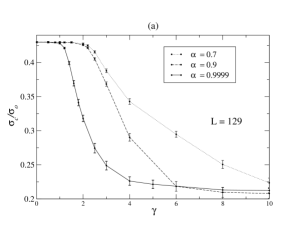
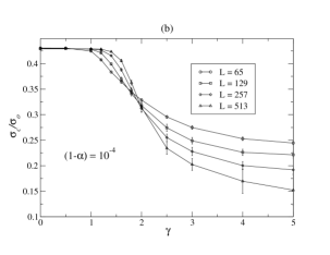
Figure 1: The ultimate strength $\frac{\sigma_{c}}{\sigma_{o}}$ of the system is studied, for a Weibull distribution of thresholds with $\rho=2$ and $\sigma_{0}=1$. a) We explore different ranges of interaction $\gamma$ and anisotropy $\alpha$. b) Results for different system sizes $L$ and ranges of interaction $\gamma$ are presented

The mechanical properties of the bundle and the statistics of internal damage events were studied numerically by varying the anisotropy strength ($\alpha$) and the range of interaction ($\gamma$). Large scale numerical simulations in $2D$ were executed. Several system sizes $(L=65,129,257,513,1025)$ were considered and simulations were performed over at least five different realizations for the biggest system $L=1025$ and five thousand for the smallest one $L=65$. We recorded the avalanche size distribution $D(\Delta)$, and the ultimate strength of the samples $\frac{\sigma_{c}}{\sigma_{o}}$, which is always normalized by the characteristic value $\sigma_{o}$ of the cumulative threshold distribution $P(\sigma)=P(\frac{\sigma}{\sigma_{o}})$ .

It is important to remark, that by using an isotropic power law stress redistribution $\Delta\sigma_{add}\sim r^{-\gamma}$, a crossover point was observed [16]. Hence, two distinct regions were distinguished, over the domain of $\gamma$. For small $\gamma$, $\frac{\sigma_{c}}{\sigma_{o}}$ is independent on $L$, which corresponds to the GLS behavior. However, when the effective range of interaction is decreased $\gamma>\gamma_{c}$, the limiting case of local load sharing is approached and the strength of the system should vanish in the $L\to\infty$ limit [24, 25]. In the isotropic case, $\gamma_{c}$ falls in the vicinity of $\gamma_{c}=2$ [16].

Figures 1a. and 1b show the critical stress values $\frac{\sigma_{c}}{\sigma_{o}}$ obtained for several ranges of interactions $\gamma$ and anisotropy strengths $\alpha$. The data corresponds to systems with $129\times 129$ elements and a Weibull distribution of breaking thresholds with $\rho=2$ and $\sigma_{o}=1$. Two distinct regions can be easily identified in the graph 1a. For small $\gamma$, the critical strength $\frac{\sigma_{c}}{\sigma_{o}}$ is independent, within statistical errors, of both the effective range of interaction $\gamma$ and the anisotropy strength $\alpha$. As we have already pointed out, this behavior is expected for the standard $GLS$ scheme. However, when the effective range of interaction decreases or the anisotropy strength increases, we found non-trivial dependencies. In Figure 1b, the critical stress of a system with strong anisotropy ($\alpha\approx 0.9999$) is detailed. We illustrate the model’s behavior for several system sizes from $L=65$ to $L=513$. For small $\gamma$, $\frac{\sigma_{c}}{\sigma_{o}}$ is independent of both effective range of interaction and system size. However, as soon as the localized nature of the interaction becomes dominant, i.e. $\gamma>\gamma_{c}$, $\frac{\sigma_{c}}{\sigma_{o}}$ vanishes logarithmically with increasing system size. This qualifies for a genuine short-range behavior as found in local load sharing models, where the strength of the sample must vanish in the thermodynamic limit [24, 25]. In summary, in the regime $\gamma\leq 1$, all the numerical findings are in excellent agreement with the mean field analytical prediction. Besides, figure 1a suggests that the crossover point $\gamma_{c}$ would differ from what was found using the isotropic stress transfer function [16] only for a very high anisotropy strength, i.e. $\alpha>0.9999$.

Nevertheless, a priori one would expect the system size dependence to be more pronounced onces the anisotropy in introduced. Figure 1b shows that in the transition region the system size dependence is more appreciable than for the isotropic case [16]. On the left side of the transition region the critical stress $\frac{\sigma_{c}}{\sigma_{o}}$ slowly increases with increasing system size. Note that for the isotropic case the convergence to the thermodynamic limit is faster; consequently, a more accurate estimation of the critical point $\gamma_{c}=2$ could be done [16]. In the present case, in order to find a reasonable estimation of $\gamma_{c}$, we used the fact that on the short range interaction region ($LLS$) the convergence to the thermodynamic limit is qualitatively different than on the long range interaction region ($GLS$). On the $GLS$ side of the transition region the critical stress $\frac{\sigma_{c}}{\sigma_{o}}$ increases with increasing system size, towards the $GLS$ exact solution. Contrary, on the $LLS$ side of the transition region $\frac{\sigma_{c}}{\sigma_{o}}$ vanishes logarithmically with increasing system size. Despite the fact that figure 1a seems to indicate $\gamma_{c}\neq 2$ for $\alpha=0.9999$, figure 1b also suggests that for any value $\alpha<1$, the critical value $\gamma_{c}$ shifts towards $\gamma_{c}=2$ as the thermodynamic limit is reached. For elucidating if the value of $\gamma_{c}$ changes onces the anisotropy is introduced we then focused on $\gamma=1$ and $\gamma=2$. Hence, changing the anisotropy strength $\alpha$ and studying the convergence of $\frac{\sigma_{c}}{\sigma_{o}}$ to the thermodynamic limit, a better estimation of $\gamma_{c}$ is done.

In Figure 2, we describe the size dependency of the ultimate strength $\frac{\sigma_{c}}{\sigma_{o}}$ for a Weibull distribution of thresholds with $\rho=2$ and $\sigma_{o}=1$. Figure 2a and figure 2b illustrate the outcomes at $\gamma=1$ and $\gamma=2$, respectively. Several anisotropy strengths were explored and it was found that when the system size is increased, the anisotropy plays a weaker role. Moreover, as expected the system size dependence is more pronounced for $\gamma=2$ than for $\gamma=1$. We note in Fig.2b that numerical uncertainties surface when one gets numerically very close to $\alpha=1$, for small system sizes. That is due to the fact that in a $2D$ square lattice topology as $\alpha\rightarrow 1$, the load sharing from one row to the next might become so small that the rows would become effectively decoupled. That is certainly an undesirable topology effect which might also magnify the system size effects. However, our results indicate that even in the presence of high anisotropy, at $\gamma_{c}=2$, the system shows a tendency to behave as $GLS$ when approaching to the thermodynamic limit, within our numerical uncertainties. Consequently, the crossover point for the anisotropic variable range of interaction given by Eq.(3) results at $\gamma_{c}=2$.

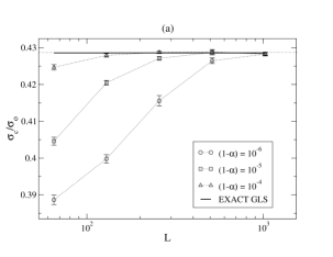
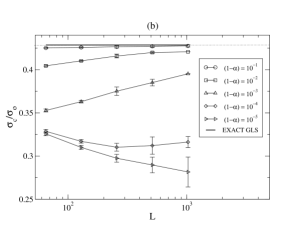
Figure 2: We show results of ultimate strength as a function of the system size, for several anisotropy strengths. A Weibull distribution of thresholds with $\rho=2$ and $\sigma_{0}=1$ is used. a) results obtained at $\gamma=1$, b) results obtained at $\gamma=2$

To test the universality of this statement, we did calculations for several threshold distributions. A Weibull distribution with $\rho=10$, as well as a uniform distribution were used for comparison. Moreover, to access accurately the crossover point, several system sizes were considered. In every case, we changed $\alpha$ using the values ($0.9;0.99;0.999$ and $0.9999$). Our aim is to elucidate how far from $GLS$ behavior the system is for $\gamma=2$, after the anisotropy is introduced. As we pointed out before, this value $\gamma_{c}=2$ defines the crossover between $GLS$ and $LLS$ behaviors, for the isotropic case.

In Figure 3, results of the ultimate strength of samples with strong anisotropy are shown in detail. The scaled magnitude $x=(\alpha_{c}-\alpha)L^{\xi}$ is plotted against the ”distance” $\delta\sigma=\sigma_{GLS}-\frac{\sigma_{c}}{\sigma_{o}}$ from the well-defined $GLS$’s behavior. Note that each symbol (i.e. square, circle and diamond) is related to a different threshold distribution. In addition, the sizes of the symbols are linked to different system sizes (the bigger the symbol, the larger the system size). Different regions of the plot, illustrated with the same symbol in five different sizes, correspond to a given value of $\alpha$ (from left to the right $0.9;0.99;0.999$ and $0.9999$). In the plots the data, corresponding to each threshold distribution, are aligned finding data collapse,

$$\delta\sigma=\left(\sigma_{GLS}-\frac{\sigma_{c}}{\sigma_{o}}\right)\sim F((\alpha_{c}-\alpha)L^{\xi})\sim F(x)$$ (6)

where we have introduced the scaling function $F((\alpha_{c}-\alpha)L^{\xi})$, with $\xi=0.5$ and $\alpha_{c}=1$.

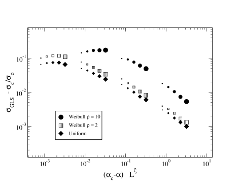
Figure 3: The ultimate strength of the system $\sigma_{c}$ is studied at $\gamma=2$, through the magnitude $\delta\sigma=\sigma_{GLS}-\frac{\sigma}{\sigma_{o}}$. Several anisotropy strength values and $(L=65,129,257,513,1025)$ are illustrated.

The results for a uniform distribution and Weibull with $\rho=2$ are very similar. Furthermore, decreasing the disorder, e.g. Weibull with $\rho=10$ and $\sigma_{o}=1$, only magnifies the topology and finite size effects. The scaling exponent $\xi\approx 0.5$ is universal, defining a new crossover exponent in $\alpha$ and $L$. From those results, one can conclude that the anisotropy does not change the crossover point for the range of interaction in 2D, $\gamma_{c}=2$. For finite systems, the global behavior is reached very slowly, as we get far from $\alpha_{c}=1$. We also notice that the distance to the $GLS$ behavior $\delta\sigma=(\sigma_{GLS}-\frac{\sigma_{c}}{\sigma_{o}})$ does vanish in the infinite system size limit, as a power law $\delta\sigma\sim L^{-\beta}$, and we estimate $\beta=0.37\pm 0.03$. We conclude, that even in presence of high anisotropy the behavior of the system for $\gamma\leq\gamma_{c}=2$ shows a tendency to $GLS$ as $L\rightarrow\infty$. The infinite system would display a qualitatively different behavior only for $\alpha_{c}=1$, where it would become effectively a $1D$ model, with $\gamma_{c}=1$.

The fracture process can also be described by the precursory activity before complete breakdown. The statistical properties of rupture sequences are characterized by the avalanche size distribution. From an experimental point of view the precursory activity is related to the acoustic emissions generated during the fracture of materials [27, 28, 29, 30]. The avalanche size distribution is a measure of causally connected broken sites. All the intact elements have a non-zero chance to fail independently of the (spatial) rupture history, and any given element could be near to its rupture point regardless of its position in the lattice.

\psfrag{AAA}{{\LARGE$\Delta^{-\frac{5}{2}}$}}\includegraphics[angle={-90},width=341.43306pt]{zap_figure4.ps}

Figure 4: Avalanche size distribution for $N=257\times 257$ fibers. Results corresponding to several anisotropic strengths are illustrated

The highly fluctuating activity is certainly related to the long range interactions where the avalanche size distribution can usually be well fitted by a power law $P(\Delta)\sim\Delta^{-\frac{5}{2}}$. This actually corresponds to the mean field scenario, $GLS$ [22, 23, 24, 25]. However, when the spatial correlations are important $LLS$, stress concentration takes place in the elements located at the perimeter of an already formed cluster. Hence, elements far away from the clusters of broken elements have significantly lower stresses and thus the size of the largest avalanche is reduced as well as the number of failed elements belonging to the same avalanche, leading to lower precursory activity.

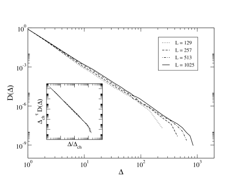
Figure 5: The normalized distributions $D(\Delta)$ of avalanches for $\alpha=0.999$ are illustrated, several system sizes are considered. In the inset we verify the scaling ansatz given by Eq.(7) with $\Delta_{ch}\sim L^{\theta}$.

Figure 4 illustrates the avalanche statistics obtained for systems with $N=257\times 257$ fibers. In every case, we have set $\gamma=2$ and used different values of the anisotropy strength $\alpha$. It is noticeable that the avalanche size distributions can always be fitted to a power law with a non-trivial exponent. However, as we get far from $\alpha=1$ the exponent tends asymptotically to the value $\tau=\frac{5}{2}$, reflecting the tendency to recover the GLS’s behavior.

To characterize the system size dependence, we propose the following scaling ansatz for the avalanche size distribution,

$$D(\Delta,L)=\Delta_{ch}^{-\tau}\,~{}g(\frac{\Delta}{\Delta_{ch}})$$ (7)

where $\Delta_{ch}$ is a characteristic avalanche $\Delta_{ch}\sim L^{\theta}$ and $g(x)$ is a scaling function that goes like $g(x)=x^{-\tau}$ for $x<1$ and decays faster than a power law for $x>1$. In Figure 5, the avalanche statistics resulting from systems with different sizes are shown. The model is again investigated at $\gamma=2$, and very strong anisotropy $\alpha=0.999$. The scaled function is presented in the inset. It can be seen that the data collapse yields $\theta=0.6\pm 0.1$ and $\tau=2.50\pm 0.02$ with a power law over several orders of magnitude in $\frac{\Delta}{\Delta_{ch}}$. This result suggests that for $\gamma=2$, even in presence of very high anisotropy, the avalanches are distributed as in the case of $GLS$, namely as $D(\Delta)\sim\Delta^{-\frac{5}{2}}$. Thus, the crossover point is still at $\gamma_{c}=2$, even in the case of an anisotropic stress redistribution (given by Eq.(3)).

4 Discussion

Long-range fiber bundle models can be considered as a first approximation to model the fracture behavior of a disordered elastic medium. It has been proposed in several instances to replace the full solution of the elastic equations by a Green function [31, 32]. This method has the advantage to avoid the computational cost involved in the inversion of the elastic equations, but in principle it is only accurate for diluted damage. A particularly simple example is provided by the random fuse model (RFM) in which a lattice of conducting bonds with random failure thresholds is loaded by applying an external voltage at the two ends of the lattice. When a fuse fails the current is redistributed to the neighboring fuses by solving the Kirchhoff equations. When only a few bonds are broken, the current is transferred according to the homogeneous lattice Green function which is given by $F(r)=x/r^{3}$ in two dimensions [31]. It is therefore a long-range (with $\gamma=2$) and anisotropic load transfer function, but of a different character than the one we have used here.

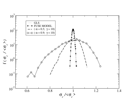
Figure 6: Global strength distribution of samples with several types of load sharing ($L=129$, averaged over 5000 different configurations). $GLS$ and $RFM$ are very the similar.

We have simulated a fiber bundle model using a load transfer function inspired by the RFM. The general result is that the failure properties of our model resemble very much those of GLS fiber bundles rather than those of the original RFM. This is particularly apparent when looking at the strength distribution, displayed in Figure  6. Both the mean-field GLS approach and our result obtained with the RFM load transfer function obey Gaussian statistics. Notice that the original RFM displays instead a qualitatively different log-normal strength distribution [3]. This confirms that the Green function approach is reliable at most in the initial stages of the damage accumulation process and it is not correct to describe the global failure of the RFM. Figure 6 also shows that anisotropic LLS functions result instead in a larger scattering of ultimate strength, and their asymmetric distributions are usually fitted by Weibull distribution functions. It is noticeable from the data that introducing very high anisotropy strength amplifies the scattering in the global strength of the samples. However, the strength distribution for the anisotropic system appears to be closer to a Gaussian in contrast to the classical Weibull behavior, which is usually obtained for LLS approaches.

In conclusion, we have studied a discrete fracture model where the interaction among elements is considered to decay anisotropically with the distance from an intact element to the rupture point. The two classical regimes (local and global) are found as the exponent of the stress-transfer function varies and a crossover point is again identified in the vicinity of $\gamma_{c}=2$. The strength of the material for $\gamma<\gamma_{c}$ does not depend on both the system size and $\gamma$ qualifying for mean-field behavior, whereas for the short range regime, the critical load vanishes in the thermodynamic limit. The behavior of the model at both sides of the crossover point was numerically studied by recording the avalanche and the critical stress for several system sizes. From our numerical results, one can certainly conclude that the anisotropy does not change the crossover point $\gamma_{c}=2$ in the 2D model, in the infinite system size limit. The $2D$ model would display a qualitatively different behavior only for $\alpha_{c}=1$, where it would become effectively a $1D$ model, with $\gamma_{c}=1$. Moreover, in finite systems for $\gamma\leq 2$, the global load sharing behavior is very slowly recovered as we get far from $\alpha_{c}=1$, within our numerical uncertainties.

5 Acknowledgments

RCH acknowledges the financial support of the Spanish Minister of Education and Science, through a Ramon y Cajal Program. This work began while the authors (RCH and SZ) were visiting the Institute for Computational Physics (ICP) at the University of Stuttgart. Its financial support and hospitality are gratefully acknowledged. HJH acknowledges the Max Planck Prize. SZ acknowledges financial support from EU FP6 NEST Pathfinder programme TRIGS under contract NEST-2005-PATH-COM-043386

References

References

- [1] Statistical Models for the Fracture of Disordered Media. Editors, H.J. Herrmann and S. Roux, North Holland (1990), and references therein.
- [2] Statistical Physics of Fracture and Breakdown in Disordered Systems. B. K. Chakrabarti, L. G. Benguigui, Clarendon Press, Oxford (1997), and references therein.
- [3] M. J. Alava, P. K. V. V. Nukala P and S. Zapperi S Adv. Phys. 55, 349 (2006)
- [4] C. Baxevanakis, D. Jeulin, J. Renard, Int. J. Fract. 73, 149 (1995).
- [5] I. J. Beyerlein, S. L. Phoenix, Eng. Fract. Mech. 57, 267 (1997).
- [6] M. Ibnabdeljalil, W. A. Curtin, Int. J. Solids Structures 34, 2649 (1997).
- [7] S. L. Phoenix, I. J. Beyerlein, Phys. Rev. E 62, 1622 (2000).
- [8] C.-L. Tsai and I. M. Daniel Int. J. Solids Structures 29 3251 (1992)
- [9] K. Anand, V. Gupta and D. Dartford, Acta Metall. Mater. 42, 797 (1994).
- [10] S. Drapier, M. R. Wisnom Composites Science and Technology 59, 2351 (1999).
- [11] H. E. Daniels, Proc. R. Soc. London A 183, 405 (1945).
- [12] B.D. Coleman, J. Appl. Phys. 28, 1058 (1957); ibid 28, 1065 (1957).
- [13] S. Zapperi, P. Ray, H. E. Stanley, A. Vespignani, Phys. Rev. Lett. 78, 1408 (1997).
- [14] W.I. Newman, D.L. Turcotte and A.M. Gabrielov,Phys. Rev. E 52, 4827 (1995).
- [15] F. Kun, S. Zapperi, H. J. Herrmann, Eur. Phys. J. B17, 269 (2000).
- [16] RC Hidalgo, Y Moreno, F Kun and H.J. Herrmann Phys. Rev. E 65, 046148 (2002).
- [17] RC Hidalgo, F Kun and H. J. Herrmann Phys. Rev. E 64, 066122 (2002).
- [18] P. Bhattacharyya, S. Pradhan, and B. K. Chakrabarti, Phys. Rev. E 67, 046122 (2003).
- [19] S. Pradhan, B. K. Chakrabarti and A Hansen Phys. Rev. E 71, 036149 (2005)
- [20] D. Sornette, J. Phys. I France 2, 2089 (1992).
- [21] W. A. Curtin, Phys. Rev. Lett. 80, 1445 (1998).
- [22] A. Hansen, P. C. Hemmer, Phys. Lett. A 184, 394 (1994).
- [23] P. C. Hemmer, A. Hansen, J. Appl. Mech. 59, 909 (1992).
- [24] D. G. Harlow, Proc. R. Soc. London A 397, 211 (1985).
- [25] M. Kloster, A. Hansen, P. C. Hemmer, Phys. Rev. E 56, 2615 (1997).
- [26] F. Raischel, F. Kun, and H. J. Herrmann Phys. Rev. E 72, 046126 (2005).
- [27] A. Garcimartin, A. Guarino, L. Bellon, S. Ciliberto, Phys. Rev. Lett. 79, 3202 (1997).
- [28] A. Guarino, A. Garcimartin, S. Ciliberto, Eur. Phys. J. B 6, 13 (1998).
- [29] C. Maes, A. van Moffaert, H. Frederix, H. Strauven, Phys. Rev. B 57, 4987 (1998).
- [30] A. Petri, G. Paparo, A. Vespignani, A. Alippi, M. Costantini, Phys. Rev. Lett. 73, 3423 (1994).
- [31] M. Barthelemy , R. da Silveira, and H. Orland, Europhys. Lett. 57, 831 (2002).
- [32] R. Toussaint and S. R. Pride, Phys. Rev. E 71, 046127 (2005).