A remark on the boundedness and convergence properties of smooth sliding mode controllers

Abstract.

Conventional sliding mode controllers are based on the assumption of switching control but a well-known drawback of this approach is the chattering phenomenon. To overcome the undesirable chattering effects, the discontinuity in the control law can be smoothed out in a thin boundary layer neighboring the switching surface. In this work, rigorous proofs of the boundedeness and convergence properties of smooth sliding mode controllers are presented. This result corrects flawed conclusions previously reached in the literature.

1. Introduction

Sliding mode control theory was conceived and developed in the former Soviet Union by Emelyanov [1], Filippov [2], Itkis [3], Utkin [5] and others. But a known drawback of conventional sliding mode controllers is the chattering phenomenon due to the discontinuous term in the control law. In order to avoid the undesired effects of the control chattering, Slotine [4] proposed the adoption of a thin boundary layer neighboring the switching surface, by replacing the sign function by a saturation function. This substitution can minimize or, when desired, even completely eliminate chattering, but turns perfect tracking into a tracking with guaranteed precision problem, which actually means that a steady-state error will always remain.

This paper presents a convergence analysis of smooth sliding mode controllers. The finite-time convergence of the tracking error vector to the boundary layer is handled using Lyapunov’s direct method. It is also analytically proven that, once in boundary layer, the error vector exponentially converges to a bounded region. This result corrects a minor flaw in Slotine’s work, by showing that the tracking error bounds are different from the bounds provided in [4].

2. Problem statement and controller design

Consider a class of $n^{\mathrm{th}}$-order nonlinear system:

(1) $$x^{(n)}=f(\mathbf{x})+b(\mathbf{x})u\\$$

where $u$ is the control input, the scalar variable $x$ is the output of interest, $x^{(n)}$ is the $n^{\mathrm{th}}$ derivative of $x$ with respect to time $t\in[0,\infty)$, $\mathbf{x}=[x,\dot{x},\ldots,x^{(n-1)}]$ is the system state vector, and $f,b:\mathbb{R}^{n}\rightarrow\mathbb{R}$ are both nonlinear functions.

In respect of the dynamic system presented in Eq. (1), the following assumptions will be made:

Assumption 1.

The function $f$ is unknown but bounded by a known function of $\mathbf{x}$, i.e., $|\hat{f}(\mathbf{x})-f(\mathbf{x})|\leq F(\mathbf{x})$ where $\hat{f}$ is an estimate of $f$.

Assumption 2.

The input gain $b(\mathbf{x})$ is unknown but positive and bounded, i.e., $0<b_{\mathrm{min}}\leq b(\mathbf{x})\leq b_{\mathrm{max}}$.

The proposed control problem is to ensure that, even in the presence of parametric uncertainties and unmodeled dynamics, the state vector $\mathbf{x}$ will follow a desired trajectory $\mathbf{x}_{d}=[x_{d},\dot{x}_{d},\ldots,x^{(n-1)}_{d}]$ in the state space.

Regarding the development of the control law the following assumptions should also be made:

Assumption 3.

The state vector $\mathbf{x}$ is available.

Assumption 4.

The desired trajectory $\mathbf{x}_{d}$ is once differentiable in time. Furthermore, every element of vector $\mathbf{x}_{d}$, as well as $x^{(n)}_{d}$, is available and with known bounds.

Now, let $\tilde{x}=x-x_{d}$ be defined as the tracking error in the variable $x$, and

$$\mathbf{\tilde{x}}=\mathbf{x}-\mathbf{x}_{d}=[\tilde{x},\dot{\tilde{x}},\ldots,\tilde{x}^{(n-1)}]$$

as the tracking error vector.

Consider a sliding surface $S$ defined in the state space by the equation $s(\mathbf{\tilde{x}})=0$, with the function $s:\mathbb{R}^{n}\rightarrow\mathbb{R}$ satisfying

$$s(\mathbf{\tilde{x}})=\left(\frac{d}{dt}+\lambda\right)^{n-1}\tilde{x}$$

or conveniently rewritten as

(2) $$s(\mathbf{\tilde{x}})=\mathbf{c^{\mathrm{T}}\tilde{x}}$$

where $\mathbf{c}=[c_{n-1}\lambda^{n-1},\ldots,c_{1}\lambda,c_{0}]$ and $c_{i}$ states for binomial coefficients, i.e.,

(3) $$c_{i}=\binom{n-1}{i}=\frac{(n-1)!}{(n-i-1)!\>i!}\>,\quad i=0,1,\ldots,n-1$$

which makes $c_{n-1}\lambda^{n-1}+\cdots+c_{1}\lambda+c_{0}$ a Hurwitz polynomial.

From Eq. (3), it can be easily verified that $c_{0}=1$, for $\forall n\geq 1$. Thus, for notational convenience, the time derivative of $s$ will be written in the following form:

(4) $$\dot{s}=\mathbf{c^{\mathrm{T}}\dot{\tilde{x}}}=\tilde{x}^{(n)}+\mathbf{\bar{c}^{\mathrm{T}}\tilde{x}}$$

where $\mathbf{\bar{c}}=[0,c_{n-1}\lambda^{n-1},\ldots,c_{1}\lambda]$.

Now, let the problem of controlling the uncertain nonlinear system (1) be treated via the classical sliding mode approach, defining a control law composed by an equivalent control $\hat{u}=\hat{b}^{-1}(-\hat{f}+x^{(n)}_{d}-\mathbf{\bar{c}^{\mathrm{T}}\tilde{x}})$ and a discontinuous term $-K\mbox{sgn}(s)$:

(5) $$u=\hat{b}^{-1}\left(-\hat{f}+x^{(n)}_{d}-\mathbf{\bar{c}^{\mathrm{T}}\tilde{x}}\right)-K\mbox{sgn}(s)$$

where $\hat{b}=\sqrt{b_{\mathrm{max}}b_{\mathrm{min}}}$ is an estimate of $b$, $K$ is a positive gain and sgn($\cdot$) is defined as

$$\mbox{sgn}(s)=\left\{\begin{array}[]{rc}-1&\mbox{if}\quad s<0\\ 0&\mbox{if}\quad s=0\\ 1&\mbox{if}\quad s>0\end{array}\right.$$

Based on Assumptions 1 and 2 and considering that $\beta^{-1}\leq\hat{b}/b\leq\beta$, where $\beta=\sqrt{b_{\mathrm{max}}/b_{\mathrm{min}}}$, the gain $K$ should be chosen according to

(6) $$K\geq\beta\hat{b}^{-1}(\eta+F)+(\beta-1)\big{|}\hat{b}^{-1}(-\hat{f}+x^{(n)}_{d}-\mathbf{\bar{c}^{\mathrm{T}}\tilde{x}})\big{|}$$

where $\eta$ is a strictly positive constant related to the reaching time.

Therefore, it can be easily verified that (5) is sufficient to impose the sliding condition

$$\frac{1}{2}\frac{d}{dt}s^{2}\leq-\eta|s|$$

which, in fact, ensures the finite-time convergence of the tracking error vector to the sliding surface $S$ and, consequently, its exponential stability.

However, the presence of a discontinuous term in the control law leads to the well known chattering effect. To avoid these undesirable high-frequency oscillations of the controlled variable, Slotine [4] proposed the adoption of a a thin boundary layer, $S_{\phi}$, in the neighborhood of the switching surface:

(7) $$S_{\phi}=\big{\{}\mathbf{x}\in\mathbb{R}^{n}\>\big{|}\>|s(\mathbf{\tilde{x}})|\leq\phi\big{\}}$$

where $\phi$ is a strictly positive constant that represents the boundary layer thickness.

The boundary layer is achieved by replacing the sign function by a continuous interpolation inside $S_{\phi}$. It should be emphasized that this smooth approximation, which will be called here $\varphi(s,\phi)$, must behave exactly like the sign function outside the boundary layer. There are several options to smooth out the ideal relay but the most common choices are the saturation function:

(8) $$\mbox{sat}(s/\phi)=\left\{\begin{array}[]{cc}\mbox{sgn}(s)&\mbox{if}\quad|s/\phi|\geq 1\\ s/\phi&\mbox{if}\quad|s/\phi|<1\end{array}\right.$$

and the hyperbolic tangent function $\tanh(s/\phi)$.

In this way, the smooth sliding mode control law can be stated as follows

(9) $$u=\hat{b}^{-1}\left(-\hat{f}+x^{(n)}_{d}-\mathbf{\bar{c}^{\mathrm{T}}\tilde{x}}\right)-K\varphi(s,\phi)$$

3. Convergence analysis

The attractiveness and invariant properties of the boundary layer are established in the following theorem.

Theorem 1.

Consider the uncertain nonlinear system (1) and Assumptions 1–4. Then, the smooth sliding mode controller defined by (9) and (6) ensures the finite-time convergence of the tracking error vector to the boundary layer $S_{\phi}$, defined according to (7).

Proof: Let a positive-definite Lyapunov function candidate $V$ be defined as

$$V(t)=\frac{1}{2}s^{2}_{\phi}$$

where $s_{\phi}$ is a measure of the distance of the current error to the boundary layer, and can be computed as follows

(10) $$s_{\phi}=s-\phi\>\mbox{sat}(s/\phi)$$

Noting that $s_{\phi}=0$ in the boundary layer, one has $\dot{V}(t)=0$ inside $S_{\phi}$. From Eqs. (8) and (10), it can be easily verified that $\dot{s}_{\phi}=\dot{s}$ outside the boundary layer and, in this case, $\dot{V}$ becomes

$$\dot{V}(t) =s_{\phi}\dot{s}_{\phi}=s_{\phi}\dot{s}=(x^{(n)}-x^{(n)}_{d}+\mathbf{\bar{c}^{\mathrm{T}}\tilde{x}})s_{\phi}$$

$$=\left(f+bu-x^{(n)}_{d}+\mathbf{\bar{c}^{\mathrm{T}}\tilde{x}}\right)s_{\phi}$$

Considering that outside the boundary layer the control law (9) takes the following form:

$$u=\hat{b}^{-1}\left(-\hat{f}+x^{(n)}_{d}-\mathbf{\bar{c}^{\mathrm{T}}\tilde{x}}\right)-K\mbox{sgn}(s_{\phi})$$

and noting that $f=\hat{f}-(\hat{f}-f)$, one has

$$\dot{V}(t)= \big{[}f+b\hat{b}^{-1}(-\hat{f}+x^{(n)}_{d}-\mathbf{\bar{c}^{\mathrm{T}}\tilde{x}})-bK\mbox{sgn}(s_{\phi})-x^{(n)}_{d}+\mathbf{\bar{c}^{\mathrm{T}}\tilde{x}}\big{]}s_{\phi}$$

$$= -\big{[}(\hat{f}-f)-b\hat{b}^{-1}(-\hat{f}+x^{(n)}_{d}-\mathbf{\bar{c}^{\mathrm{T}}\tilde{x}})+(-\hat{f}+x^{(n)}_{d}-\mathbf{\bar{c}^{\mathrm{T}}\tilde{x}})+bK\mbox{sgn}(s_{\phi})\big{]}s_{\phi}$$

So, considering Assumptions 1 and 2 and defining $K$ according to (6), $\dot{V}$ becomes:

$$\dot{V}(t)\leq-\eta|s_{\phi}|$$

which implies $V(t)\leq V(0)$ and that $s_{\phi}$ is bounded. From the definition of $s_{\phi}$, it can be easily verified that $s$ is bounded. Considering Assumption 4 and Eq. (4), it can be concluded that $\dot{s}$ is also bounded.

The finite-time convergence of the tracking error vector to the boundary layer can be shown by recalling that

$$\dot{V}(t)=\frac{1}{2}\frac{d}{dt}s_{\phi}^{2}=s_{\phi}\dot{s}_{\phi}\leq-\eta|s_{\phi}|$$

Then, dividing by $|s_{\phi}|$ and integrating both sides between 0 and $t$ gives

$$\int^{t}_{0}\frac{s_{\phi}}{|s_{\phi}|}\dot{s}_{\phi}\,d\tau\leq-\int^{t}_{0}\eta\,d\tau$$

$$|s_{\phi}(t)|-|s_{\phi}(0)|\leq-\eta\,t$$

In this way, considering $t_{\mathrm{reach}}$ as the time required to hit $S_{\phi}$ and noting that $|s_{\phi}(t_{\mathrm{reach}})|=0$, one has

$$t_{\mathrm{reach}}\leq\frac{|s_{\phi}(0)|}{\eta}$$

which guarantees the convergence of the tracking error vector to the boundary layer in a time interval smaller than $|s_{\phi}(0)|/\eta$ and completes the proof. $\square$

Therefore, the value of the positive constant $\eta$ can be properly chosen in order to keep the reaching time, $t_{\mathrm{reach}}$, as short as possible. Figure 1 shows that the time evolution of $|s_{\phi}|$ is bounded by the straight line $|s_{\phi}(t)|=|s_{\phi}(0)|-\eta\,t$.

Figure 1. Time evolution of $|s_{\phi}|$.

Finally, the proof of the boundedness of the tracking error vector relies on Theorem 2.

Theorem 2.

Let the boundary layer $S_{\phi}$ be defined according to (7). Then, once inside $S_{\phi}$, the tracking error vector will exponentially converge to a closed region $\Phi=\{\mathbf{x}\in\mathbb{R}^{n}\>|\>|s(\mathbf{\tilde{x}})|\leq\phi\mbox{ and }|\tilde{x}^{(i)}|\leq\zeta_{i}\lambda^{i-n+1}\phi,i=0,1,\ldots,n-1\}$, with $\zeta_{i}$ defined as

(11) $$\zeta_{i}=\left\{\begin{array}[]{cl}1&\mbox{for}\quad i=0\\ 1+\sum^{i-1}_{j=0}\binom{i}{j}\zeta_{j}&\mbox{for}\quad i=1,2,\ldots,n-1.\end{array}\right.$$

Proof: From the definition of $s$, Eq. (2), and considering that $|s(\mathbf{x})|\leq\phi$ may be rewritten as $-\phi\leq s(\mathbf{x})\leq\phi$, one has

(12) $$-\phi\leq c_{0}\tilde{x}^{(n-1)}+c_{1}\lambda\tilde{x}^{(n-2)}+\cdots+c_{n-1}\lambda^{n-1}\tilde{x}\leq\phi$$

Multiplying (12) by $e^{\lambda t}$ yields

(13) $$-\phi e^{\lambda t}\leq\frac{d^{n-1}}{dt^{n-1}}(\tilde{x}e^{\lambda t})\leq\phi e^{\lambda t}$$

Integrating (13) between $0$ and $t$ gives

(14) $$-\frac{\phi}{\lambda}e^{\lambda t}+\frac{\phi}{\lambda}\leq\frac{d^{n-2}}{dt^{n-2}}(\tilde{x}e^{\lambda t})-\left.\frac{d^{n-2}}{dt^{n-2}}(\tilde{x}e^{\lambda t})\right|_{t=0}\leq\frac{\phi}{\lambda}e^{\lambda t}-\frac{\phi}{\lambda}$$

or conveniently rewritten as

(15) $$-\frac{\phi}{\lambda}e^{\lambda t}-\left(\left|\frac{d^{n-2}}{dt^{n-2}}(\tilde{x}e^{\lambda t})\right|_{t=0}+\frac{\phi}{\lambda}\right)\\ \leq\frac{d^{n-2}}{dt^{n-2}}(\tilde{x}e^{\lambda t})\leq\\ \frac{\phi}{\lambda}e^{\lambda t}+\left(\left|\frac{d^{n-2}}{dt^{n-2}}(\tilde{x}e^{\lambda t})\right|_{t=0}+\frac{\phi}{\lambda}\right)$$

The same reasoning can be repeatedly applied until the $(n-1)^{\mathrm{th}}$ integral of (13) is reached:

(16) $$-\frac{\phi}{\lambda^{n-1}}e^{\lambda t}-\left(\left|\frac{d^{n-2}}{dt^{n-2}}(\tilde{x}e^{\lambda t})\right|_{t=0}+\frac{\phi}{\lambda}\right)\frac{t^{n-2}}{(n-2)!}-\cdots\\ -\left(\left|\tilde{x}(0)\right|+\frac{\phi}{\lambda^{n-1}}\right)\leq\tilde{x}e^{\lambda t}\leq\frac{\phi}{\lambda^{n-1}}e^{\lambda t}+\\ \left(\left|\frac{d^{n-2}}{dt^{n-2}}(\tilde{x}e^{\lambda t})\right|_{t=0}+\frac{\phi}{\lambda}\right)\frac{t^{n-2}}{(n-2)!}+\cdots+\left(\left|\tilde{x}(0)\right|+\frac{\phi}{\lambda^{n-1}}\right)$$

Furthermore, dividing (16) by $e^{\lambda t}$, it can be easily verified that, for $t\to\infty$,

(17) $$-\frac{\phi}{\lambda^{n-1}}\leq\tilde{x}(t)\leq\frac{\phi}{\lambda^{n-1}}$$

Considering the $(n-2)^{\mathrm{th}}$ integral of (13)

(18) $$-\frac{\phi}{\lambda^{n-2}}e^{\lambda t}-\left(\left|\frac{d^{n-2}}{dt^{n-2}}(\tilde{x}e^{\lambda t})\right|_{t=0}+\frac{\phi}{\lambda}\right)\frac{t^{n-3}}{(n-3)!}-\cdots\\ -\left(\left|\dot{\tilde{x}}(0)\right|+\frac{\phi}{\lambda^{n-2}}\right)\leq\frac{d}{dt}(\tilde{x}e^{\lambda t})\leq\frac{\phi}{\lambda^{n-2}}e^{\lambda t}+\\ \left(\left|\frac{d^{n-2}}{dt^{n-2}}(\tilde{x}e^{\lambda t})\right|_{t=0}+\frac{\phi}{\lambda}\right)\frac{t^{n-3}}{(n-3)!}+\cdots+\left(\left|\dot{\tilde{x}}(0)\right|+\frac{\phi}{\lambda^{n-2}}\right)$$

and noting that $d(\tilde{x}e^{\lambda t})/dt=\dot{\tilde{x}}e^{\lambda t}+\tilde{x}\lambda e^{\lambda t}$, by imposing the bounds (17) to (18) and dividing again by $e^{\lambda t}$, it follows that, for $t\to\infty$,

(19) $$-2\frac{\phi}{\lambda^{n-2}}\leq\dot{\tilde{x}}(t)\leq 2\frac{\phi}{\lambda^{n-2}}$$

Now, applying the bounds (17) and (19) to the $(n-3)^{\mathrm{th}}$ integral of (13) and dividing once again by $e^{\lambda t}$, it follows that, for $t\to\infty$,

(20) $$-6\frac{\phi}{\lambda^{n-3}}\leq\ddot{\tilde{x}}(t)\leq 6\frac{\phi}{\lambda^{n-3}}$$

The same procedure can be successively repeated until the bounds for $\tilde{x}^{(n-1)}$ are achieved:

(21) $$-\left(1+\sum^{n-2}_{i=0}\binom{n-1}{i}\zeta_{i}\right)\phi\leq\tilde{x}^{(n-1)}\leq\left(1+\sum^{n-2}_{i=0}\binom{n-1}{i}\zeta_{i}\right)\phi$$

where the coefficients $\zeta_{i}$ ($i=0,1,\ldots,n-2$) are related to the previously obtained bounds of each $\tilde{x}^{(i)}$ and can be summarized as in (11).

In this way, by inspection of the integrals of (13), as well as (17), (19), (20), (21) and the other omitted bounds, it follows that the tracking error will be confined within the limits $|\tilde{x}^{(i)}|\leq\zeta_{i}\lambda^{i-n+1}\phi,i=0,1,\ldots,n-1$, where $\zeta_{i}$ is defined by (11).

However, the aforementioned bounds define an $n$-dimensional box that is not completely inside the boundary layer. Figure. 2 illustrates for a $2^{\mathrm{nd}}$-order system ($n=2$).

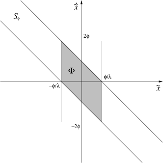
Figure 2. Bounds of $x^{(i)}$ for a $2^{\mathrm{nd}}$-order system.

Considering the attractiveness and invariant properties of $S_{\phi}$ demonstrated in Theorem 1, the region of convergence can be stated as the intersection of the boundary layer and the $n$-dimensional box defined by the preceding bounds. Therefore, it follows that the tracking error vector will exponentially converge to a closed region $\Phi=\{\mathbf{x}\in\mathbb{R}^{n}\>|\>|s(\mathbf{\tilde{x}})|\leq\phi\mbox{ and }|\tilde{x}^{(i)}|\leq\zeta_{i}\lambda^{i-n+1}\phi,i=0,1,\ldots,n-1\}$, with $\zeta_{i}$ defined by (11). $\square$

Remark 1.

Theorem 2 corrects a minor error in [4]. Slotine proposed that the bounds for $\tilde{x}^{(i)}$ could be summarized as $|\tilde{x}^{(i)}|\leq 2^{i}\lambda^{i-n+1}\phi,i=0,1,\ldots,n-1$. Although both results lead to same bounds for $\tilde{x}$ and $\dot{\tilde{x}}$, they start to differ from each other when the order of the derivative is higher than one, $i>1$. For example, according to Slotine the bounds for the second derivative would be $|\ddot{\tilde{x}}|\leq 4\phi\lambda^{3-n}$ and not $|\ddot{\tilde{x}}|\leq 6\phi\lambda^{3-n}$, as demonstrated in Theorem 2.

4. Concluding remarks

In this work, a convergence analysis of smooth sliding mode controllers was presented. The attractiveness and invariant properties of the boundary layer as well as the exponential convergence of the tracking error vector to a bounded region were analytically proven. This last result corrected flawed conclusions previously reached in the literature.

References

[1] S. V. Emelyanov and N. E. Kostyleva. Design of variable structure systems
with discontinuous switching function. Engineering Cybernetics, 21(1):156–160, 1964.
[2] A. F. Filippov. Differential equations with discontinuous right-hand side.
American Mathematical Society Translations, 42(2):199–231, 1964.
[3] U. Itkis. Control Systems of Variable Structure. Wiley, New York, 1976.
[4] J.-J. E. Slotine. Sliding controller design for nonlinear systems. International Journal of Control, 40(2):421–434, 1984.
[5] V. I. Utkin. Variable structure systems with sliding modes. IEEE
Transactions on Automatic Control, 22(2):212–220, 1977.