BROWN-HET 1493

We study the six-dimensional dilaton gravity Yang black holes of [1], which carry $(1,-1)$ charge in $SU(2)\times SU(2)$ gauge group. We find what values of the asymptotic parameters (mass and scalar charge) lead to a regular horizon, and show that there are no regular solutions with an extremal horizon.

1 Introduction

The canonical charged black hole is the Reissner–Nordström (RN) solution. For a given charge and mass, the no-hair theorem guarantees it is the only static solution of Einstein–Maxwell theory in four spacetime dimensions. It can carry magnetic monopole charge, with its singularity hidden behind a horizon, which non-gravitating objects cannot do without a naked singularity. It has both an inner and outer horizon (an event horizon, and an inner Cauchy horizon) which merge in the extremal limit $Q=M$, leading to an $AdS$ throat geometry.

It is interesting to consider the generalization to nonabelian gauge groups. Without gravity, theories with nonabelian gauge groups have Yang monopoles, which like their Dirac cousins are singular [2, 3]. But when the gauge group is spontaneously broken, there are non-singular ’t Hooft–Polyakov monopoles [4, 5]. Adding gravity, one can place a small Schwarzschild black hole at the centre of one of these, to produce one of Weinberg’s hairy black holes [6, 7, 8]. These can have identical mass and charge to the RN solutions, which still exist in the larger theory, hence forming classical hair. Gravity also allows other regular solutions which do not exist in flat space [9].

String theory encourages us to examine theories in more than four dimensions, possibly with a dilaton. Extra dimensions allow black holes to have novel features, such as multiple angular momenta [10] and non-spherical horizon topology [11, 12]. Adding charge, [13] study $SO(2k+1)$ gauge theory in $2k+2$ dimensions, with gravity. This includes RN as the $k=1$ case, and the $k=2$ case also has a double horizon and an extremal limit. See also [14, 15].

In addition to these string-inspired solutions, there are some which arise more directly in string theory. Fundamental heterotic strings can end on certain monopoles, [16, 17] and various kinds of D-branes can end on others [18, 19, 20]. In this paper, we study the case of Bergshoeff, Gibbons & Townsend [1] in which an M5-brane connects two M9-branes which are separated along the 11th direction. Taking the 10-dimensional view, there are 4 dimensions along the intersection, 6 perpendicular to it, and a dilaton. The two M5-M9 intersections give opposite charges in two copies of $SU(2)$, which are superimposed. The same monopole can also be constructed using instead the D-branes of type IIA string theory [21].

Section 2 sets up the problem, and recalls the asymptotic expansion given by [1]. In Section 3 we find a near-horizon expansion, and connect this to a subspace of the parameter space at infinity. Section 4 examines a singular case, and finally Section 5 studies the solution near the singularity, connecting this to the near-horizon solution as a check that nothing unexpected happens in between.

2 Asymptotic Behaviour

The action for 6-dimensional dilaton gravity with a Yang-Mills field is [1]

$$S=\int d^{6}x\sqrt{-\det g}\left[R-(\partial\sigma)^{2}-4\kappa e^{-\sigma}\mathrm{tr}\left|F^{2}\right|\right]$$

and we immediately choose units such that $\kappa=1$. Write the metric as

$$ds^{2}=-e^{2\lambda}\Delta dt^{2}+\frac{dr^{2}}{\Delta}+r^{2}d\Omega^{2}$$ (1)

in terms of two functions of the radial co-ordinate, $\lambda(r)$ and $\Delta=1-2\mu(r)/r^{3}$.

We take the gauge group to be $SU(2)\times SU(2)$. Yang monopoles may then have charges in one or both factors. For monopole with charge $(1,-1)$, $\mathrm{tr}\left|F^{2}\right|=6/r^{4}$ and the equations of motion become [1]

$$0 =\Delta r^{4}\sigma^{\prime\prime}+\left(4r^{3}-2\mu-6e^{-\sigma}r\right)\sigma^{\prime}+12e^{-\sigma}$$

$$0 =\mu^{\prime}-3e^{-\sigma}-\Delta r^{4}(\sigma^{\prime})^{2}/8$$ (2)

$$0 =4\lambda^{\prime}-(\sigma^{\prime})^{2}r\,.$$

The third equation simply fixes $\lambda$ in terms of $\sigma$, up to one constant, which is an overall scaling of $t.$ Whenever an aymptotic region exists, we fix this by demanding $\lambda(\infty)=0$. The meat is in the first two equations, which are second order in $\sigma$ and first in $\mu$, thus we need 3 other boundary conditions.

Reference [1] gives the following asymptotic solution for large $r$, with three parameters $\sigma_{0}$, $\mu_{0}$ and $\Sigma$:

$$\sigma =\sigma_{0}+\frac{A}{r^{2}}+\frac{\Sigma}{r^{3}}+\frac{A^{2}}{2r^{4}}+\ldots$$

$$\mu =\frac{Ar}{2}+\mu_{0}-\frac{A\Sigma}{2r^{2}}-\frac{4A^{3}+9\Sigma^{2}}{24r^{3}}+\ldots$$ (3)

$$\lambda =-\frac{A^{2}}{r^{4}}-\frac{3A\Sigma}{5r^{5}}+\ldots\qquad\qquad\qquad\mbox{with }A=6e^{-\sigma_{0}}\,.$$

Notice in the above equations of motion that the existence of a regular horizon ($\Delta(r_{H})=0$ with $\Delta r^{4}\sigma^{\prime\prime}=0$) imposes one relation between $\sigma^{\prime}$ and $\mu$ at $r_{H}$, thus reducing the number of free parameters by one. Thus one would expect only a two-parameter family of these asymptotic solutions to lead to a regular horizon. In the next section we find these solutions.

3 Near the Regular Horizon

To find solutions with a regular horizon, we assume its existence at $r=r_{H}$ and expand in $d=r-r_{H}$. This leads to the following near-horizon solution, with two parameters $r_{H}$ and $\sigma_{H}$ (plus a third, $\lambda_{H}$, which is fixed by $\lambda(\infty)=0$):

$$\mu =\frac{r_{H}^{3}}{2}+\frac{A_{H}}{2}d+\frac{3A_{H}^{2}}{4r_{H}(3r_{H}^{2}-A_{H})}d^{2}+\ldots$$

$$\sigma =\sigma_{H}-\frac{2A_{H}}{r_{H}(3r_{H}^{2}-A_{H})}d+\frac{A^{3}-12A_{H}^{2}r_{H}^{2}+18Ar_{H}^{4}}{r_{H}^{2}(3r_{H}^{2}-A_{H})^{3}}d^{2}+\ldots$$ (4)

$$\lambda =\lambda_{H}+\frac{A_{H}^{2}}{r_{H}(3r_{H}^{2}-A_{H})^{2}}d+\ldots\qquad\qquad\qquad\mbox{with }A_{H}=6e^{-\sigma_{H}}\,.$$

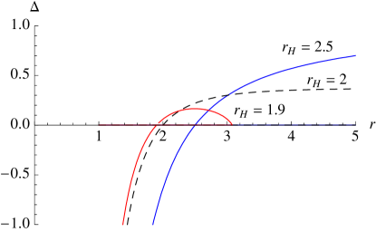
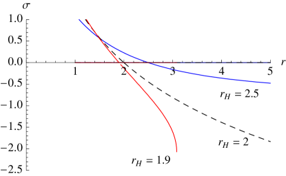
Figure 1: Plots of $\Delta(r)$ and $\sigma(r)$ for three values of $r_{H}$, all with $\sigma_{H}=0$. They are $r_{H}=1.9$ (red), $r_{H}=2$ (dashed) and $r_{H}=2.5$ (blue, extending to $r=\infty$).

Given one solution, we can generate another by scaling by a factor $\gamma$: the new functions defined by

$$\bar{\mu}(\bar{r}) =\frac{\mu(\gamma\bar{r})}{\gamma^{3}}\qquad\mbox{i.e. }\bar{\Delta}(\bar{r})=\Delta(\gamma\bar{r})$$

$$\bar{\sigma}(\bar{r}) =\sigma(\gamma\bar{r})+2\log\gamma$$ (5)

$$\bar{\lambda}(\bar{r}) =\lambda(\gamma\bar{r})$$

obey the same equations. Starting with the near-horizon solution $(r_{H},\sigma_{H})$, the new solution will have parameters

$$(\bar{r}_{H},\bar{\sigma}_{H})=(r_{H}/\gamma\,,\>\sigma_{H}+2\log\gamma).$$ (7)

We can set $\bar{\sigma}_{H}=0$ by taking $\gamma=e^{-\sigma_{H}/2}$. Thus we may focus on the case $\sigma_{H}=0$ ($A_{H}=6$) without loss of generality.

The behavior of this solution is different in three ranges of $r_{H}$:

• $r_{H}<\sqrt{2}$ implies $\Delta^{\prime}<0$ at the horizon, so this cannot be the outermost horizon (as $\Delta=1$ at infinity).

• $\sqrt{2}<r_{H}<2$ leads to a singular space: at some finite $r=r_{M}$, $\Delta\to 0$ and $\sigma^{\prime}\to-\infty$, producing a curvature singularity. This is discussed in the next section.

• $r_{H}>2$ matches onto the asymptotic solution (3), with $\Delta\to 1$ as $r\to\infty$.

Figure 1 shows the second and third cases, and the boundary between them.

We now study the third case. Since an asymptotic region exists, we can fix $\lambda_{H}$ using $\lambda(\infty)=0$. The remaining near-horizon parameters $(r_{H},\sigma_{H})$ are mapped to a two dimensional subspace of $(\mu_{0},\Sigma,\sigma_{0})$ at infinity. Focusing on the $\sigma_{H}=0$ case, $r_{H}$ is mapped to a line. The first part of Figure 2 shows these parameters along this line.

The scaling (6), acting on the asymptotic solution’s parameters, reads

$$(\bar{\mu}_{0},\bar{\Sigma},\bar{\sigma}_{0})=(\gamma^{-3}\mu_{0}\,,\>\gamma^{-3}\Sigma,\>\sigma_{0}+2\log\gamma).$$ (8)

Just as we could at the horizon, we can set $\bar{\sigma}_{0}=0$ by taking $\gamma=e^{-\sigma_{0}/2}$. Then the line of parameters connecting to a regular horizon $r_{H}>2$ becomes a line in the $(\bar{\mu}_{0},\bar{\Sigma})$ plane. The second part of Figure 2 shows this curve. Asymptotic solutions with (scaled) parameters not on this curve have a naked singularity at the origin.

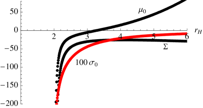
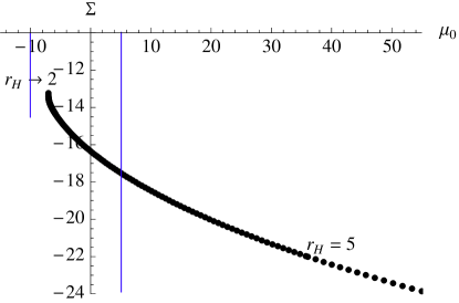
Figure 2: Parameters of the asymptotic solution (3) connecting to near-horizon solution (4) with $\sigma_{H}=0$. On the left, $\mu_{0}$, $\Sigma$ and $100\sigma_{0}$ (in red) against $r_{H}$. On the right, the scaling (8) has been used to set $\sigma_{0}$ to zero, and $\Sigma$ is plotted against $\mu_{0}$. The blue lines are regions investigated in section 5 below.

4 Closed Geometry, a singular case

Here we study the second case above, $\sqrt{2}<r_{H}<2$, in which $\Delta$ appears to have a second zero outside the regular horizon.

Begin by changing co-ordinates from $r$ to radial distance $y$:

$$ds^{2}=-a(y)\,dt^{2}+dy^{2}+r(y)^{2}d\Omega^{2}$$ (9)

replacing $\lambda(r)$, $\mu(r)$ and $\sigma(r)$ with new functions $a(y)$, $r(y)$ and $\sigma(y)$. Among other relationships between them,

$$\Delta(r)=\left(\frac{dr}{dy}\right)^{2}\qquad\mbox{ and }\qquad\sigma^{\prime}(r)=\frac{d\sigma}{dy}\bigg{/}\frac{dr}{dy}.$$

Thus a maximum of $r(x)$, with $\sigma(x)$ regular, will lead to $\Delta=0$ and $\sigma^{\prime}(r)$ diverging, which is what happens in Figure 1.

Placing $y=0$ at this point, we expand and find the following series solution with parameters $r_{M}$, $\sigma_{M}$ and $\sigma_{2}$:

$$r =r_{M}-\frac{3(2A_{M}-r_{M}^{2})}{2r_{M}^{2}}y^{2}+\ldots\qquad\qquad\mbox{with }A_{M}=6e^{-\sigma_{M}}$$

$$\sigma =\sigma_{M}+\frac{\sqrt{12}\sqrt{2A_{M}-r_{M}^{2}}}{r_{M}^{2}}y+\frac{\sigma_{2}}{2}y^{2}+\ldots$$ (10)

$$a =4\log\left|y\right|+a_{M}-\frac{2r_{M}\sigma_{2}}{\sqrt{3}\sqrt{2A_{M}-r_{M}^{2}}}y+\ldots\,.$$

This matches the numerical solution very well. So as far as the first two of equations (2) are concerned, the apparent divergences at $r_{M}$ are simply due to this being a maximum radius for the transverse sphere, beyond which $r$ is no longer a valid co-ordinate.

But the third equation (for $\lambda$, or $a$) then leads us to a different interpretation: since $a=-g_{00}$ diverges, the point $r_{M}$ is in fact a curvature singularity. Hence we discard these solutions.

5 Near the Singularity

We claimed above that for generic values of the asymptotic parameters (i.e. those not on the curve of Figure 2) there is a naked singularity, and that there is never a second horizon inside the regular horizon studied.

Here we justify these claims by connecting the near-horizon and asymptotic solutions to another approximate solution near the singularity at $r=0$. This is the following:

$$\sigma =\alpha\log r+\sigma_{Z}+\ldots$$

$$\mu =\frac{\beta}{r^{\alpha^{2}/4}}+\frac{12e^{-\sigma_{Z}}\>r^{1-\alpha}}{(\alpha-2)^{2}}+\frac{\alpha^{2}\>r^{3}}{2(\alpha^{2}+12)}+\ldots$$ (11)

$$\lambda =\frac{\alpha^{2}}{4}\log r+\lambda_{Z}+\ldots\,.$$

(We discuss further corrections to this in the Appendix.)

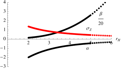
Figure 3: Parameters of the solution near the singularity (11) connecting to near-horizon solution (4) with $\sigma_{H}=0$. On the left, $\alpha$, $\beta/20$ and $\sigma_{Z}$ (in red). On the right, the scaling (12) has been used to set $\sigma_{Z}$ to zero, and we now plot $\overline{\beta}$ against $\alpha$ for $2<r_{H}<20$.

Just as we integrated outwards to connect the near-horizon solution to the asymptotic solution above, we can integrate inwards and connect it to the solution near the singularity. Figure 3 is analogous to Figure 2.

Acting on this solution’s parameters, the scaling (6) now reads

$$(\overline{\alpha},\overline{\beta},\overline{\sigma}_{Z})=\left(\alpha,\frac{\beta}{\gamma^{3+\alpha^{2}/4}},\sigma_{Z}+(2+\alpha)\log\gamma\right).$$ (12)

Thus demanding $\overline{\sigma}_{Z}=0$ rescales $\beta$ to $\overline{\beta}=e^{-\frac{\sigma_{Z}}{1+\alpha}\left(3+\frac{\alpha^{2}}{4}\right)}\beta$.

We can also start far away, with the asymptotic solution, and integrate in to the singularity. For each point on $(\mu_{0},\Sigma)$ plane of Figure 2 not on the curve drawn there, we do not encounter a horizon before reaching the singularity. Figure 4 shows the resulting parameters near the singularity, taking points $(\mu_{0},\Sigma)$ along the two vertical lines drawn on Figure 2. These show the generic behaviour, either crossing the curve of solutions with a regular horizon (at $\mu_{0}=5$) or avoiding it (at $\mu_{0}=-10$).

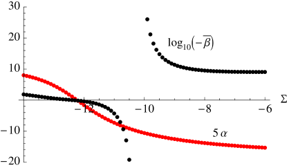
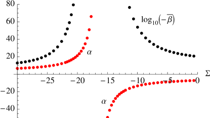
Figure 4: Parameters of the solution near the singularity (11) connecting to asymptotic solution (3) with $\sigma_{0}=0$. These follow the two blue lines on Figure 2. On the left, $\mu_{0}=-10$, where there is never a horizon, and on the right, $\mu_{0}=5$, crossing the curve of solutions with a regular horizon at $\Sigma\approx-17$. The scaled parameter $\bar{\beta}$ is large and negative, so we plot $\log_{10}(-\bar{\beta})$, and $5\alpha$ or $\alpha$ (in red).
Note that, on the left, the point at which $\bar{\beta}$ diverges is $\alpha=-2$. This is $c_{1}=\alpha+2=0$, in terms of the parameter used in the Appendix.

6 Conclusions

At spatial infinity the solution appears to have three parameters, but since there is one scaling relationship, we can focus on two: $\mu_{0}$ and $\Sigma$. Further restricting to solutions with a regular horizon, we find a one-parameter family of solutions, with horizon at $r=r_{H}\geq\sqrt{2}$. Only those with $r_{H}>2$ connect smoothly to spatial infinity, which excludes the extremal case.

Numerically integrating outwards from the horizon, we find the curve in the $(\mu_{0},\Sigma)$ plane of points which describe black holes. Integrating inwards from the horizon, we arrive at a singularity at $r=0$ without encountering another horizon. Starting at infinity, from a point in the $(\mu_{0},\Sigma)$ plane not on the curve, we can again integrate inwards all the way to the singularity at $r=0$, showing that there isn’t another class of horizons.

Thus we concluded that the horizon structure of the 6-dimensional black holes studied in [1] is like that of Schwarzschild; unlike Reissner–Nordström and the six-dimensional Yang black holes of [13] it does not have an inner horizon nor an extremal limit.

Appendix A Correction near the Singularity

For the asymptotic solution (3) and the near-horizon solution (4), it is clear that the next terms are higher powers of $\frac{1}{r}$ or $d$, which are easy to calculate and obviously smaller than the terms written. But for the solution (11) near $r=0$ things are not so simple. This appendix finds a correction to this, in different variables, and shows that the remainder is small in the appropriate limit.

We can combine the first two of equations (2) into one third-order equation for $\sigma(r)$ alone by solving the second for $\mu^{\prime}(r)$ and substituting this into $\partial_{r}$ of the first. The result is the quotient of a third-order and a second-order differential equation

$$\frac{\mathcal{N}[\sigma^{\prime\prime},\sigma^{\prime},\sigma]}{\mathcal{D}[\sigma^{\prime},\sigma]}=0$$

where the numerator and denominator are:

$$\mathcal{N} =r^{2}\left(e^{\sigma}r^{2}-2\right)\sigma^{\prime 4}+r\left(\left(e^{\sigma}r^{2}-2\right)\sigma^{\prime\prime}r^{2}+12\right)\sigma^{\prime 3}$$

$$\quad+4\left(4e^{\sigma}r^{2}+3\sigma^{\prime\prime}r^{2}-8\right)\sigma^{\prime 2}-4r\left(e^{\sigma}r^{2}-2\right)\left(r\sigma^{\prime\prime\prime}-4\sigma^{\prime\prime}\right)\sigma^{\prime}$$

$$\qquad-32\sigma^{\prime\prime}+8r\left(r\left(e^{\sigma}r^{2}-2\right)\sigma^{\prime\prime 2}-2\sigma^{\prime\prime\prime}\right)\,,$$

$$\mathcal{D} =\frac{4}{3}e^{\sigma}\left(\sigma^{\prime}+r\sigma^{\prime\prime}\right)\,.$$

In (11) we had $\sigma(r)=\alpha\log r+\sigma_{Z}$, which sets both $\mathcal{N}$ and $\mathcal{D}$ to zero. We will refer to this as the singular solution.

We now seek a solution of $\mathcal{N}=0$ alone. This equation is equivalent to the following nonlinear second-order equation:

$$0= (-128x^{3}+32x^{4})b+(32x^{2}-8x^{3})b^{2}-(24x-6x^{2})b^{3}+(2-x)b^{4}$$ (13)

$$+\left[128x^{4}-32x^{5}+(32x^{2}-10x^{3})b^{2}-(2x-x^{2})b^{3}\right]b^{\prime}$$

$$+\left[-32x^{4}+8x^{5}-(8x^{3}-4x^{4})b\right]b^{\prime 2}+\left[(-32x^{4}+8x^{5})b+(8x^{3}-4x^{4})b^{2}\right]b^{\prime\prime}$$

where the new function $b(x)$ is related to $\sigma(r)$ by

$$e^{\sigma(r)}=\frac{x(r)}{r^{2}},\qquad r(x)=e^{\int\frac{1}{b(x)}dx+c_{3}}\,.$$ (14)

One solution of this is $b_{0}(x)=c_{1}x$, leading to $\sigma(r)=(c_{1}-2)\log r-c_{1}c_{3}$, the singular solution. To find a correction to this, we make the ansatz

$$b(x)=c_{1}x\left(1+\int_{x_{0}}^{x}p(x^{\prime})dx^{\prime}\right)$$ (15)

and expand in $p$. Write the second order equation (13) as

$$0=\mathcal{A}[p(x)]+\mathcal{B}[p(x)]$$

where $\mathcal{A}$ is the term linear in $p$, and $\mathcal{B}$ is the nonlinear piece. The linear equation $\mathcal{A}[p(x)]=0$ is

$$0 =c_{1}(c_{1}-4)x^{5}\left((8-6c_{1})(x-4)+c_{1}^{2}(x-2)\right)p(x)$$

$$\quad+4c_{1}^{2}x^{6}\left(8-2x+c_{1}(x-2)\right)p^{\prime}(x)$$

which can be integrated to give

$$p_{1}(x)=c_{2}\,x^{\frac{c_{1}}{4}+\frac{4}{c_{1}}}\left(\frac{1}{x^{2}}(c_{1}-2)-\frac{2}{x^{3}}(c_{1}-4)\right)\,.$$

When substituting back into the ansatz (15) for $b(x)$, the coefficient of $x$, initially $c_{1}$, will in general be renormalized by the term from the lower limit of integration. Keeping this coefficient free of $c_{2}$ will keep the power $x^{\frac{c_{1}}{4}+\frac{4}{c_{1}}}$ independent of $c_{2}$, allowing for a simple $c_{2}\to 0$ limit. To do this, we take

$$x_{0}=\frac{2c_{1}^{2}-8c_{1}+32}{(c_{1}-4)(c_{1}-2)}$$

and then obtain

$$b(x) =c_{1}x+c_{2}x^{\frac{c_{1}}{4}+\frac{4}{c_{1}}}\left(\frac{4c_{1}^{2}(c_{1}-2)}{16+c_{1}(c_{1}-4)}+\frac{1}{x}\,\frac{8c_{1}^{2}}{4-c_{1}}\right)\,.$$ (16)

This is, implicitly, an approximate solution for $\sigma(r)$ with three parameters $c_{1}$, $c_{2}$ and $c_{3}$, thus cannot be a solution to $\mathcal{D}=0$ for generic values. We can match it to numerical $\sigma(r)$ using (14).

The variable $x$ can be either large or small near $r=0$, depending on the sign of $c_{1}$. From (14), we have $x(r)=r^{2}e^{\sigma(r)}\sim r^{2}r^{\alpha}=r^{c_{1}}$. When $c_{1}>0$, $x\to 0$ as $r\to 0$. This occurs behind the regular horizon (see Figure 3) and also for the naked singularity, when $\Sigma\lesssim-10$ and $\Sigma\lesssim-10$ in Figure 4’s first and second graphs. In the solution $b_{1}(x)$ above, the power $\frac{c_{1}}{4}+\frac{4}{c_{1}}$ is at least 2, thus the $c_{2}$ correction terms die faster than the unperturbed term $c_{1}x$.

When $c_{1}<0$, then instead $x\to\infty$ as $r\to 0$. This occurs for the other half of 4a. The power $\frac{c_{1}}{4}+\frac{4}{c_{1}}$ is now negative, so the $c_{2}$ correction terms are small at large $x$, while the unperturbed term is large.

Finally, we perform a check that this approximation $p_{1}(x)$ to the nonlinear solution is a good one. Define a Green’s function $\mathcal{A}[G(x,y)]=\delta(x-y)$. Then the full solution is

$$p(x)=p_{1}(x)-\int dy\,G(x,y)\,\mathcal{B}[p(y)]\,.$$

For $x<1$, the Green’s function is

$$G(x,y) =\frac{8-2x+c_{1}(x-2)}{4c_{1}^{2}\left(8-2y+c_{1}(y-2)\right)^{2}x^{3}y^{3}}\left(\frac{x}{y}\right)^{\frac{c_{1}}{4}+\frac{4}{c_{1}}}\quad\mbox{when }x<y<1\mbox{, else zero}$$

$$\sim x^{-3}x^{\frac{c_{1}}{4}+\frac{4}{c_{1}}}\>y^{-3}y^{-(\frac{c_{1}}{4}+\frac{4}{c_{1}})}\quad\mbox{as }x,y\to 0$$

and we approximate the full nonlinear kernel $\mathcal{B}[p(y)]$ by the known $\mathcal{B}[p_{1}(y)]$ to obtain the next order correction. We find

$$\mathcal{B}[p_{1}(y)]\sim\left(y^{\frac{c_{1}}{4}+\frac{4}{c_{1}}}\right)^{2}\quad\mbox{as }y\to 0\,.$$

Thus the nonlinear corrected solution looks like

$$p(x) \sim p_{1}(x)-x^{-3}x^{\frac{c_{1}}{4}+\frac{4}{c_{1}}}\int_{x}^{1}dy\,y^{-3}y^{\frac{c_{1}}{4}+\frac{4}{c_{1}}}+\ldots$$

$$\sim x^{-3}x^{\frac{c_{1}}{4}+\frac{4}{c_{1}}}\left(1+x^{-2}x^{\frac{c_{1}}{4}+\frac{4}{c_{1}}}+\ldots\right)\,.$$

Since $\frac{c_{1}}{4}+\frac{4}{c_{1}}>2$ (for $c_{1}\neq 4$) this is a small correction to the linear piece in the limit $x\to 0$.

For $x>1$, the Green’s function is

$$G(x,y) =-\frac{8-2x+c_{1}(x-2)}{4c_{1}^{2}\left(8-2y+c_{1}(y-2)\right)^{2}x^{3}y^{3}}\left(\frac{x}{y}\right)^{\frac{c_{1}}{4}+\frac{4}{c_{1}}}\quad\mbox{when }1<y<x\mbox{, else zero}$$

$$\sim x^{-2}x^{\frac{c_{1}}{4}+\frac{4}{c_{1}}}\>y^{-4}y^{-(\frac{c_{1}}{4}+\frac{4}{c_{1}})}\quad\mbox{as }x,y\to\infty$$

and the leading power in $\mathcal{B}$ is now

$$\mathcal{B}[p_{1}(y)]\sim y^{3}\left(y^{\frac{c_{1}}{4}+\frac{4}{c_{1}}}\right)^{2}\quad\mbox{as }y\to\infty\,.$$

This time the corrected solution is

$$p(x) \sim p_{1}(x)-x^{-2}x^{\frac{c_{1}}{4}+\frac{4}{c_{1}}}\int_{1}^{x}dy\,y^{-2}y^{\frac{c_{1}}{4}+\frac{4}{c_{1}}}+\ldots$$

$$\sim x^{-2}x^{\frac{c_{1}}{4}+\frac{4}{c_{1}}}\left(1+x^{-1}x^{\frac{c_{1}}{4}+\frac{4}{c_{1}}}+\ldots\right)$$

The nonlinear piece is now a very small correction in the limit $x\to\infty$, as $\frac{c_{1}}{4}+\frac{4}{c_{1}}<-2$.

References

[1]
E. A. Bergshoeff, G. W. Gibbons, and P. K. Townsend, “Open m5-branes,” Phys. Rev. Lett.97 (2006) 231601,
hep-th/0607193.
[2]
P. A. M. Dirac, “Quantised singularities in the electromagnetic field,” Proc. Roy. Soc. Lond.A133 (1931)
60–72.
[3]
C. N. Yang, “Generalization of dirac’s monopole to su(2) gauge fields,” J. Math. Phys.19 (1978)
320.
[4]
G. ’t Hooft, “Magnetic monopoles in unified gauge theories,” Nucl.
Phys.B79 (1974)
276–284.
[5]
A. A. Belavin, A. M. Polyakov, A. S. Shvarts, and Y. S. Tyupkin,
“Pseudoparticle solutions of the yang-mills equations,” Phys. Lett.B59 (1975)
85–87.
[6]
K.-M. Lee and E. J. Weinberg, “Charged black holes with scalar hair,” Phys. Rev.D44 (1991)
3159–3163.
[7]
K.-M. Lee, V. P. Nair, and E. J. Weinberg, “Black holes in magnetic
monopoles,” Phys. Rev.D45 (1992) 2751–2761,
hep-th/9112008.
[8]
E. J. Weinberg, “Black holes with hair,”
gr-qc/0106030.
[9]
R. Bartnik and J. Mckinnon, “Particle - like solutions of the einstein
yang-mills equations,” Phys. Rev. Lett.61 (1988)
141–144.
[10]
R. C. Myers and M. J. Perry, “Black holes in higher dimensional space-times,”
Ann. Phys.172 (1986)
304.
[11]
R. Emparan and H. S. Reall, “A rotating black ring in five dimensions,” Phys. Rev. Lett.88 (2002) 101101,
hep-th/0110260.
[12]
H. Elvang and P. Figueras, “Black Saturn,” JHEP05 (2007) 050,
hep-th/0701035.
[13]
G. W. Gibbons and P. K. Townsend, “Self-gravitating yang monopoles in all
dimensions,” Class. Quant. Grav.23 (2006) 4873–4886,
hep-th/0604024.
[14]
D.-f. Zeng, W.-s. Xu, and Y.-h. Gao, “Yang-type monopoles in 5 dimensional
curved space-time,”
hep-th/0605077.
[15]
T. Tchrakian, “Dirac-yang monopoles and their regular counterparts,”
hep-th/0612249.
[16]
J. Polchinski, “Open heterotic strings,” JHEP09 (2006) 082,
hep-th/0510033.
[17]
O. Bergman and G. Lifschytz, “When d-branes break,” Phys. Lett.B641 (2006)
88–93.
[18]
A. Strominger, “Open p-branes,” Phys. Lett.B383 (1996) 44–47,
hep-th/9512059.
[19]
P. K. Townsend, “D-branes from M-branes,” Phys. Lett.B373
(1996) 68–75,
hep-th/9512062.
[20]
D. S. Berman, “M-theory branes and their interactions,” Phys. Rept.456 (2008) 89–126,
arXiv:0710.1707
[hep-th].
[21]
A. Belhaj, P. Diaz, and A. Segui, “On the superstring realization of the yang
monopole,”
hep-th/0703255.