Solving the Bethe-Salpeter equation for a pseudoscalar meson in Minkowski space

V. Šauli CFTP and Departamento de Física, Instituto Superior Técnico, Av. Rovisco Pais, 1049-001 Lisbon, Portugal, Department of Theoretical Physics, Nuclear Physics Institute, Řež near Prague, CZ-25068, Czech Republic
Abstract

A new method of solution of the Bethe-Salpeter equation for a pseudoscalar quark-antiquark bound state is proposed. With the help of an integral representation, the results are directly obtained in Minkowski space. Dressing of Green’s functions is naturally taken into account, thus providing the possible inclusion of a running coupling constant as well as quark propagators. First numerical results are presented for a simplified ladder approximation.

pacs:
11.10.St, 11.15.Tk

I Introduction

Among the various approaches used in meson physics, the formalism of Bethe-Salpeter and Dyson-Schwinger equations (DSEs) plays a traditional and indispensable role. The Bethe-Salpeter equation (BSE) provides a field-theoretical starting point to describe hadrons as relativistic bound states of quarks and/or antiquarks. For instance, the DSE and BSE framework has been widely used in order to obtain nonperturbative information about the spectra and decays of the whole lightest pseudoscalar nonet, with an emphasis on the QCD pseudo-Goldstone boson — the pion PSEUDO . Moreover, the formalism satisfactorily provides a window to the ’next-scale’ meson sector, too, including vector, scalar SCALARY and excited mesons. Finally, electromagnetic form factors of mesons have been calculated with this approach for space-like momenta FORMFAKTORY .

When dealing with bound states composed of light quarks, then it is unavoidable to use the full covariant BSE framework. Nonperturbative knowledge of the Green’s function, which makes part of the BSE kernel, is required. Very often, the problem is solved in Euclidean space, where it is more tractable, as there are no Green’s function singularities there. The physical amplitudes can be then obtained by continuation to Minkowski space. Note that the extraction of mass spectra is already a complicated task BHKRW2007 , not to speak of an analytic continuation of Euclidean-space form factors.

When dealing with heavy quarkonia or mixed heavy mesons like $B_{c}$ (found at Fermilab by the CDF Collaboration BCmesons ), some simplifying approximations are possible. Different approaches have been developed to reduce the computational complexity of the full four-dimensional (4D) BSE. The so-called instantaneous INSTA and quasi-potential approximations QUASI can reduce the 4D BSE to a 3D equation in a Lorentz-covariant manner. In practice, such 3D equations are much more tractable, since their resolution is less involved, especially if one exploits the considerable freedom in performing the 3D reduction. Also note that, contrary to the BSE in the ladder approximation, these equations reduce to the Schrödinger equation of nonrelativistic Heavy-Meson Effective Theory and nonrelativistic QCD HEAVY . However, the interaction kernels of the reduced equations often correspond to input based on economical phenomenological models, and the connection to the underlying theory (QCD) is less clear (if not abandoned from the onset).

In the present paper, we extend the method of solving the full 4D BSE, originally developed for pure scalar theories NAKAN ; KUSIWI ; SAUADA2003 , to theories with nontrivial spin degrees of freedom. Under a certain assumption on the functional form of Green’s functions, we develop a method of solving the BSE directly in Minkowski space, in its original manifestly Lorentz-covariant 4D form. In order to make our paper as self-contained as possible, we shall next supply some basic facts about the BSE approach to relativistic mesonic bound states.

The crucial step to derive the homogeneous BSE for bound states is the assumption that the bound state reflects itself in a pole of the four-point Green’s function for on-shell total momentum $P$, with $P^{2}=M_{j}^{2}$, viz.

$$G^{(4)}(p,p^{\prime},P)=\sum_{j}\frac{-i}{(2\pi)^{4}}\frac{\psi_{j}(p,P_{os})\bar{\psi_{j}}(p^{\prime},P_{os})}{2E_{p_{j}}(P^{0}-E_{p_{j}}+i\epsilon)}+\mbox{regular terms}\;,$$ (1)

where $E_{p_{j}}=\sqrt{\vec{p}\,{}^{2}+M_{j}^{2}}$ and $M_{j}$ is the (positive) mass of the bound state characterized by the BS wave function $\psi_{j}$ carrying the set of quantum numbers $j$. Then the BSE can be conventionally written in momentum space like

$\displaystyle S_{1}^{-1}(p_{+},P)\psi(p,P)S_{2}^{-1}(p_{-},P)$ $\displaystyle=-i\int\frac{d^{4}k}{(2\pi)^{4}}V(p,k,P)\psi(p,P)\,,$ (2)
$\displaystyle p_{+}$ $\displaystyle=p+\alpha P\,,$
$\displaystyle p_{-}$ $\displaystyle=p-(1-\alpha)P\,,$

or, equivalently, in terms of BS vertex function $\Gamma$ as

$\displaystyle\Gamma(p,P)$ $\displaystyle=$ $\displaystyle-i\int\frac{d^{4}k}{(2\pi)^{4}}V(p,k,P)S_{1}(k_{+},P)\Gamma(p,P)S_{2}(k_{-},P)\,,$ (3)

where we suppress all Dirac, flavor and Lorentz indices, and $\alpha\in(0,1)$. The function $V$ represents the two-body-irreducible interaction kernel, and $S_{i}$ ($i=1,2$) are the dressed propagators of the constituents. The free propagators read

$$S_{i}^{0}(p)=\frac{\not p+m_{i}}{p^{2}-m^{2}_{i}+i\epsilon}.$$ (4)

Concerning solutions to the BSE (3) for pseudoscalar mesons, they have the generic form LEW

$$\Gamma(q,P)=\gamma_{5}[\Gamma_{A}+\Gamma_{B}q.P\not\!q+\Gamma_{C}\not\!P+\Gamma_{D}\not\!q\not\!P+\Gamma_{E}\not\!P\not\!q],$$ (5)

where the $\Gamma_{i}$, with $i=A,B,C,D,E$, are scalar functions of their arguments $P,q$. If the bound state has a well-defined charge parity, say ${\cal{C}}=1$, then these functions are even in $q.P$, and furthermore $\Gamma_{D}=-\Gamma_{E}$.

As was already discussed in Ref. MUNCZEK , the dominant contribution to the BSE vertex function for pseudoscalar mesons comes from the first term in Eq. (5). This is already true, at a 15% accuracy level, for the light pseudoscalars $\pi,K,\eta$, while in the case of ground-state heavy pseudoscalars, like the $\eta_{c}$ and $\eta_{b}$, the contributions from the other tensor components in Eq. (5) are even more negligible. Hence, at this stage of our Minkowski calculation, we also approximate our solution by taking $\Gamma=\gamma_{5}\Gamma_{A}$.

The interaction kernel is approximated by the dressed gluon propagator, with the interaction gluon-quark-antiquark vertices taken in their bare forms. Thus, we may write

$$V(p,q,P)=g^{2}(\kappa)D_{\mu\nu}(p-q,\kappa)\gamma^{\nu}\otimes\gamma^{\mu}\,,$$ (6)

where the full gluon propagator is renormalized at a scale $\kappa$. The effective running strong coupling $\alpha_{s}$ is then related to $g$ through the equations

$\displaystyle g^{2}(\kappa)D_{\mu\nu}(l,\kappa)$ $\displaystyle=\alpha_{s}(l,\kappa)\frac{P^{T}_{\mu\nu}(l)}{l^{2}+i\epsilon}-\xi g^{2}(\kappa)\frac{l_{\mu}l_{\nu}}{l^{4}+i\epsilon}\,,$ (7)
$\displaystyle\alpha_{s}(q,\kappa)$ $\displaystyle=\frac{g^{2}(\kappa)}{1-\Pi(q^{2},\kappa)}\,,$
$\displaystyle P^{T}_{\mu\nu}(l)$ $\displaystyle=-g_{\mu\nu}+\frac{l_{\mu}l_{\nu}}{l^{2}}\,.$

From the class of $\xi$-linear covariant gauges, the Landau gauge $\xi=0$ will be employed throughout the present paper.

In the next section, we shall derive the solution for the dressed-ladder approximation to the BSE, i.e., all propagators are considered dressed ones, and no crossed diagrams are taken into account. The BSE for quark-antiquark states has many times been treated in Euclidean space, even beyond the ladder approximation. Most notably, the importance of dressing the proper vertices in the light-quark sector was already stressed in Ref. ACHJO , so our approximations are certainly expected to have a limited validity. Going beyond the rainbow ($\gamma_{\mu}$) approximation is straightforward but rather involved. (For comparison, see the Minkowski study of Schwinger-Dyson equations published in Refs. SAULIJHEP ; SAULI2 ), the latter paper including the minimal-gauge covariant vertex instead of the bare one). In the present paper, we prefer to describe the computational method rather than carrying out a BSE study with the most sophisticated kernel known in the literature.

The set-up of this paper is as follows. In Sec. 2 we describe the method of solving the BSE. As a demonstration, numerical results are presented in Sec. 3. Conclusions are drawn in Sec. 4. The detailed derivations of the integral equation, that we actually solved numerically, are presented in the Appendices.

II Integral representation and solution of the BSE

In this section we describe our method of solving the BSE in Minkowski space. It basically assumes that the various Green’s functions appearing in the interaction kernel can be written as weighted integrals over the various spectral functions (i.e., the real distribution) $\rho$.

More explicitly stated, the full quark and gluon propagators, the latter ones in the Landau gauge, are assumed to satisfy the standard Lehmann representation, which reads

$$S(l)=\int_{0}^{\infty}d\omega\frac{\rho_{v}(\omega)\not l+\rho_{s}(\omega)}{l^{2}-\omega+i\epsilon}\,,$$ (8)
$$G_{\mu\nu}(l)=\int_{0}^{\infty}d\omega\frac{\rho_{g}(\omega)}{l^{2}-\omega+i\epsilon}P^{T}_{\mu\nu}(l)\,,$$ (9)

where $\rho$ is a real istribution. Until now, with certain limitations, the integral representations  (8) and (9) have been used for the nonperturbative evaluation of Green’s functions in various models SAFBP . However, we should note here that the true analytic structure of QCD Green’s functions is not reliably known (also see Refs. ALKSME ; FISHER1 ; SABIA ), which studies suggests the tructure given by  (8) and (9) is not sufficient if not excluded. In this case, the lehmann representation or perhaps the ussage of real $\rho$ in the integral representation  (8) and (9) can be regarded as an analyticized approximation of the true quark propagator. The complexification of $rho$ within the complex integration path is one of the straightforward and questionable generalization ARRBRO . The general question of the existence of Lehamnn represintation in QCD is beyond the scope of presented paper and we do not discussed the problem furthermore.

Furthermore, we generalize here the idea of the Perturbation Theory Integral Representation (PTIR) NAKAN , specifically for our case. The PTIR represents a unique integral representation (IR) for an $n$-point Green’s function defined by an $n$-leg Feynman integral. The generalized PTIR formula for the $n$-point function in a theory involving fields with arbitrary spin is exactly the same as in the original scalar theory considered in Ref. NAKAN , but the spectral function now acquires a nontrivial tensor structure. Let us denote such a generalized weight function by $\rho(\alpha,x_{i})$. Then, it can be clearly decomposed into the sum

$$\rho(\alpha,x_{i})_{\mbox{\scriptsize scalar theory}}\rightarrow\sum_{j}\rho_{j}(\alpha,x_{i}){\cal{P}}_{j},$$ (10)

where $\alpha,x_{i}$ represent the set of spectral variables, and $j$ runs over all possible independent combinations of Lorentz tensors and Dirac matrices $P_{j}$. The function $\rho_{j}(\alpha,x_{i})$ just represents the PTIR weight function of the $j$-th form factor (the scalar function by definition), since it can obviously be written as a suitable scalar Feynman integral. Leaving aside the question of (renormalization) scheme dependence, we refer the reader to the textbook by Nakanishi NAKAN for a detailed derivation of the PTIR. The simplest examples of such ”generalized” integral representations corresponds with Lehmann representations for spin half  (8) and spin one propagators (9).

Let us now apply our idea to the pseudoscalar bound-state vertex function keeping in mind that the singularity structure (given by the denominators) of the r.h.s. of the BSE is the same as in the scalar models studied in Refs. KUSIWI ; SAUADA2003 , the appropriate IR for the pseudoscalar bound- state vertex function $\Gamma_{A}(q,P)$ should read

$$\Gamma_{A}(q,P)=\int_{0}^{\infty}d\omega\int_{-1}^{1}dz\frac{\rho_{A}^{[N]}(\omega,z)}{\left[F(\omega,z;P,q)\right]^{N}}\,,$$ (11)

where we have introduced a useful abbreviation for the denominator of the IR (11), viz.

$$F(\omega,z;P,q)=\omega-(q^{2}+q.Pz+P^{2}/4)-i\epsilon\,,$$ (12)

with $N$ a free integer parameter.

Substituting the IRs (11), (9), (8) into the r.h.s. of the BSE (3), one can analytically integrate over the loop momenta. Assuming the uniqueness theorem NAKAN , we should arrive at the same IR (11), because of the r.h.s. of the BSE (3). The derivation is given in Appendix A for the cases $N=1,2$.

In other words, we have converted the momentum BSE (with a singular kernel) into a homogeneous two-dimensional integral equation for the real weight function $\rho_{A}^{[N]}(\omega,z)$, i.e.,

$$\rho^{[N]}_{A}(\tilde{\omega},\tilde{z})=\int_{0}^{\infty}d\omega\int_{-1}^{1}dzV^{[N]}(\tilde{\omega},\tilde{z};\omega,z)\rho^{[N]}_{A}(\omega,z),$$ (13)

where the kernel $V^{[N]}(\tilde{\omega},\tilde{z};\omega,z)$ is a regular multivariable function.

The kernel $V^{[N]}$ also automatically supports the domain $\Omega$ where the function $\rho^{[N]}_{A}(\omega,z)$ is nontrivial. This domain is always smaller then the infinite strip $[0,\infty)\times[-1,1]$, as is explicitly assumed by the boundaries of the integrals over $\omega$ and $z$. For instance, with the simplest kernel parametrized by a free gluon propagator and constituent quarks of mass $m$, we get for the flavor-singlet meson $\rho^{[N]}_{A}(\omega,z)\neq 0$ only if $\omega>m^{2}$.

In our approach, to solve the momentum BSE in Minkowski space is equivalent to finding a real solution to the real integral equation (13). No special choice of frame is required. If one needs the resulting vertex function, can be obtained by numerical integration over $\rho_{N}$ in an arbitrary reference frame.

III Numerical Results

In this section we discuss the numerical solution of the BSE with various interaction kernels. For that purpose, we shall vary the coupling strength as well as the effective gluon mass $m_{g}$. We are mainly concerned with the range of binding energies that coincide with those of heavy quarkonia, which systems we shall study in future work. Moreover, we take a discrete set of values for the mass $m_{g}$, such that it runs from zero to the value of the constituent quark mass. These values are expected to be relevant for the case of a true gluon propagator (when $m_{g}$ is replaced by the continuous spectral variable $\omega$ (9)). Thus, in each case, the corresponding gluon density is $\rho_{g}(c)=N_{g}\delta(c-m^{2}_{g})$, which specifies the kernel of the BSE to be (in the Landau gauge)

$$V(q-p)=g^{2}\frac{-g_{\mu\nu}+\frac{(q-p)_{\mu}(q-p)_{\nu}}{(q-p)^{2}}}{(q-p)^{2}-m_{g}^{2}+i\epsilon}\gamma^{\nu}\otimes\gamma^{\mu}$$ (14)

where the prefactor (including the trace of the color matrices) is simply absorbed in the coupling constant. For our actual calculation, we use the bare constituent propagator $S_{i}(p_{i})$ with heavy quark mass $M\equiv m$ (see Appendix A for this approximation).

Firstly, we follow the standard procedure: after fixing the bound-state mass ($\sqrt{P^{2}}$), we look for a solution by iterating the BSE for a spectral function with fixed coupling constant $\alpha=g^{2}/(4\pi)$. Very similarly to the scalar case SAUADA2003 , the choice $N=2$ for the power of $F$ in the IR of the bound-state vertex function is the preferred one. This choice is a reasonable compromise between on the one hand limiting numerical errors and on the other hand avoiding the computational obstacles for high $N$. Here we note that using $N=1$ is rather unsatisfactory (comparing with the massive Wick-Cutkosky model), since then we do not find any stable solution for a wide class of input parameters $g$, $m_{g}$. In contrast, using the value $N=2$ we obtain stable results for all possible interaction kernels considered here. This includes the cases with vanishing $m_{g}$, which means that the numerical problems originally present in the scalar models SAUADA2003 are fully overcome here. The details of our numerical treatment are given in Appendix B.

As is more usual in the nonrelativistic case, we fix the coupling constant $\alpha=g^{2}/(4\pi)$ and then look for the bound-state mass spectrum. We find the same results in either case, whether $P$ or $\alpha$ is fixed first, noting however that in the latter case the whole integration in the kernel $K$ needs to be carried out in each iteration step, which makes the problem more computer-time consuming.

Refer to caption

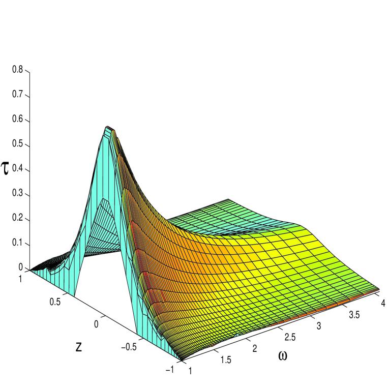
Figure 1: The rescaled weight function $\tau=\frac{\rho^{[2]}(\omega,z)}{\omega^{2}}$ for the following model parameters: $\eta=0.95$, $m_{g}=0.001M$, $\alpha_{s}=0.666$; the small mass $m_{g}$ approximates the one-gluon-exchange interaction kernel.

The obtained solutions for varying $\alpha$ and mass $m_{g}$, with a fixed fractional binding $\eta=\sqrt{P^{2}}/(2M)=0.95$, are given in Table 1. If we fix the gluon mass at $m_{g}=0.5$ and vary the fractional binding $\eta$, we obtain the spectrum of Table 2.

$m_{g}/m_{q}$ $10^{-3}$ 0.01 0.1 0.5
$\alpha$ 0.666 0.669 0.745 1.029

TABLE 1. Coupling constant $\alpha_{s}=g^{2}/(4\pi)$ for several choices of $m_{g}/M$, with given binding fraction $\eta=\sqrt{P^{2}}/(2M)=0.95$.

$\eta:$ 0.8 0.9 0.95 0.99
$\alpha$ 1.20 1.12 1.03 0.816

TABLE 2. Coupling $\alpha_{s}=g^{2}/(4\pi)$ as a function of binding fraction $\eta=\sqrt{P^{2}}/(2M)$, for exchanged massive gluon with $m_{g}=0.5M$.

For illustration, the weight function $\tilde{\rho}^{[2]}$ is displayed in Fig. 1.

IV Summary and Conclusions

The main result of the present paper is the development of a technical framework to solve the bound-state BSE in Minkowski space. In order to obtain the spectrum, no preferred reference frame is needed, and the wave function can be obtained in an arbitrary frame — without numerical boosting — by a simple integration of the weight function.

The treatment is based on the usage of an IR for the Green’s functions of a given theory, including the bound-state vertices themselves. The method has been explained and checked numerically on the samples of pseudoscalar fermion-antifermion bound states. It was shown that the momentum-space BSE can be converted into a real equation for a real weight functions $\rho$, which is easily solved numerically. The main motivation of the author was to develop a practical tool respecting selfconsistency of DSEs and BSEs. Generalizing this study to other mesons, such as vectors and scalars, and considering more general flavor or isospin structures, with the simultaneous improvement of the approximations (correctly dressed gluon propagator, dressed vertices, etc.), will be an essential step towards a fully Lorentz-covariant description of a plethora of transitions and form factors in the time-like four-momentum region.

Acknowledgments

I would like to thank George Rupp for his careful reading of the manuscript.

Appendix A Kernel Functions

With the Dirac indices explicitly written out, the BSE for quark-antiquark bound states reads

$$\Gamma(q,P)_{\omega\rho}=i\int\frac{d^{4}q}{(2\pi)^{4}}S(q+P/2)_{\beta\gamma}\Gamma(q,P)_{\gamma\gamma^{\prime}}S(q-P/2)_{\gamma^{\prime}\beta^{\prime}}V_{\omega\beta\beta^{\prime}\rho}(q,k;P),$$ (15)

where the Lorentz indices of the vertex function have not been specified.

In our approximation, the IR for a pseudoscalar bound-state vertex function is

$$\Gamma(q,P)^{\alpha\beta}=\gamma_{5}^{\alpha\beta}\int_{0}^{\infty}d\omega\int_{-1}^{1}dz\frac{\rho^{[N]}(\omega,z)}{\left[F(\omega,z;P,q)\right]^{N}},$$ (16)

and the generalized kernel for the BSE in the ladder approximation has the form

$$V_{\alpha\beta\gamma\delta}=g^{2}\int_{0}^{\infty}dc\frac{-g_{\mu\nu}+\frac{(q-p)_{\mu}(q-p)_{\nu}}{(q-p)^{2}}}{(q-p)^{2}-c+i\epsilon}\rho_{g}(c)\gamma^{\nu}_{\alpha\beta}\gamma^{\mu}_{\gamma\delta},$$ (17)

where the indices $\alpha,\beta,\gamma,\delta$ and $\mu,\nu$ stand for the appropriate Dirac and Lorentz structures, respectively. Moreover, we use the IR for all functions entering the BSE, including the vertex (16), the kernel (17), and the propagators $S(q_{\pm})$ (8).

For the purpose of brevity, we shall use the following abbreviation for the prefactor:

$$\int_{\cal{S}}\equiv-3\int_{0}^{\infty}d\omega\int_{-1}^{+1}dz\int_{0}^{\infty}dc\int_{0}^{\infty}da\int_{0}^{\infty}db\rho^{[N]}(\omega,z)g^{2}\rho_{g}(c)\,.$$ (18)

With this convention, the BSE can be written as

$\displaystyle\int d\tilde{\omega}d\tilde{z}\frac{\rho^{N}(\tilde{\omega},\tilde{z})}{\left[F(\tilde{\omega},\tilde{z};p,P)\right]^{N}}=i\int_{\cal{S}}\int\frac{d^{4}q}{(2\pi)^{4}}\frac{\rho_{v}(a)\rho_{v}(b)(q^{2}-P^{2}/4)-\rho_{s}(a)\rho_{s}(b)}{\left[F(\omega,z;q,P)\right]^{N}D_{1}D_{2}D_{3}}\,,$ (19)

where the trace is taken over the Dirac indices (after multiplying by $\gamma_{5}$), and where

$\displaystyle D_{1}$ $\displaystyle=$ $\displaystyle(q+P/2)^{2}-a+i\epsilon\,,$
$\displaystyle D_{2}$ $\displaystyle=$ $\displaystyle(q-P/2)^{2}-b+i\epsilon\,,$
$\displaystyle D_{3}$ $\displaystyle=$ $\displaystyle(q-p)^{2}-c+i\epsilon\,.$ (20)

In the following, we shall transform the r.h.s. of the BSE (19) into its IR, i.e., the l.h.s. of Eq. (19).

As a first step, we use the algebraic identities

$$\frac{q^{2}}{F(\omega,z;q,P)}=\frac{\omega-q.Pz-P^{2}/4}{F(\omega,z;q,P)}-1\,,$$
$$\frac{q.P}{D_{1}D_{2}}=\frac{1}{2}\left(\frac{1}{D_{1}}-\frac{1}{D_{2}}+\frac{b-a}{D_{1}D_{2}}\right)\,,$$ (21)

which gives us for the r.h.s. of Eq. (19)

$\displaystyle i\int_{\cal{S}}\int\frac{d^{4}q}{(2\pi)^{4}}\left\{\frac{-\frac{z}{2}\rho_{v}(a)\rho_{v}(b)}{\left[F(\omega,z;q,P)\right]^{N}D_{3}}\left(\frac{1}{D_{1}}-\frac{1}{D_{2}}\right)\right.$ (22)
$\displaystyle+$ $\displaystyle\frac{(\omega-P^{2}/2+\frac{a-b}{2}z)\rho_{v}(a)\rho_{v}(b)-\rho_{s}(a)\rho_{s}(b)}{\left[F(\omega,z;q,P)\right]^{N}D_{1}D_{2}D_{3}}-\frac{\rho_{v}(a)\rho_{v}(b)}{\left[F(\omega,z;q,P)\right]^{N-1}D_{1}D_{2}D_{3}}.$

Furthermore, we employ Feynman parametrization, starting with the first term in expression (22), which yields

$\displaystyle\frac{1}{\left[F(\omega,z;q,P)\right]^{N}}\left(\frac{1}{D_{1}}-\frac{1}{D_{2}}\right)=(-)^{N}\int_{0}^{1}dx\frac{\Gamma(N+1)x^{N-1}}{\Gamma(N)}$
$\displaystyle\left\{\left[q^{2}+q.P(zx-(1-x))+P^{2}/4-\omega x-a(1-x)\right]^{-N-1}\right.$
$\displaystyle-\left.\left[q^{2}+q.P(zx+(1-x))+P^{2}/4-\omega x-b(1-x)\right]^{-N-1}\right\}\,.$ (23)

Substituting Eq. (A) back into expression (22), using the Feynman variable $y$ so as to match the scalar propagator $D_{3}$, and integrating over the four-momentum $q$, we get for the first line in expression (22)

$\displaystyle(-)^{N-1}\int_{\cal{S}}\frac{\rho_{v}(a)\rho_{v}(b)}{2(4\pi)^{2}}\int_{0}^{1}dx\int_{0}^{1}dyy^{N}x^{1-N}z$
$\displaystyle\left\{\left[\frac{P^{2}}{4}\left[y-y^{2}(x(1+z)-1)^{2}\right]+q^{2}(1-y)y+P.py(1-y)(x(1+z)-1)-U(a)\right]^{-N}\right.$
$\displaystyle-\left.\left[\frac{P^{2}}{4}\left[y-y^{2}(x(z-1)+1)^{2}\right]+q^{2}(1-y)y+P.py(1-y)(x(z-1)+1)-U(b)\right]^{-N}\right\},$

where we have defined

$$U(a)=\left[\omega x+a(1-x)\right]y+c(1-y)\,.$$ (25)

Making the substitution $x\rightarrow\tilde{z}$, such that $\tilde{z}=x(1+z)-1$ in the second line of expression (A), we can write for the first term in the large bracket (A) (including all prefactors of the first line  (A))

$\displaystyle(-)\frac{\int_{\cal{S}}}{(4\pi)^{2}}\int_{0}^{1}dy\int_{-1}^{z}d\tilde{z}\left(\frac{1+\tilde{z}}{1+z}\right)^{N-1}\frac{z}{1+z}\frac{\rho_{v}(a)\rho_{v}(b)}{2(1-y)^{N}\left[F(\tilde{\Omega},\tilde{z};p,P)\right]^{N}}\,,$ (26)

where $F$ is defined in Eq. (12), and where

$$\tilde{\Omega}=\frac{\left(\omega\frac{1+\tilde{z}}{1+z}+a\frac{z-\tilde{z}}{1+z}\right)y+c(1-y)-\frac{P^{2}}{4}y^{2}(1-\tilde{z}^{2})}{y(1-y)}\,.$$ (27)

Introducing the identity

$$1=\int_{0}^{\infty}d\tilde{\omega}\delta(\tilde{\omega}-\tilde{\Omega})$$ (28)

into the expression (26), changing the integral ordering, and integrating over the Feynman variable $y$, we arrive at the desired expression for  (26)

$\displaystyle\int_{0}^{\infty}d\tilde{\omega}\int_{-1}^{1}d\tilde{z}\frac{\chi_{1}(\tilde{\omega},\tilde{z})}{\left[F(\tilde{\omega},\tilde{z};p,P)\right]^{N}};$
$\displaystyle\chi_{1}(\tilde{\omega},\tilde{z})=-\int_{\cal{S}}\frac{T_{+}^{N-1}}{2(4\pi)^{2}}\frac{z\rho_{v}(a)\rho_{v}(b)}{1+z}\theta(z-\tilde{z})\sum_{j=\pm}\frac{y_{aj}\theta(D_{a})\theta(y_{aj})\theta(1-y_{aj})}{(1-y_{aj})^{N-1}\sqrt{D_{a}}}\,,$ (29)

where $y_{a\pm}$ are the roots of the quadratic equation

$$y^{2}A+yB_{a}+c=0,$$ (30)

with the functions $A,B_{a},D_{a}$ defined as

$\displaystyle A=\tilde{\omega}-S;\hskip 28.45274ptB_{a}=(\omega-a)T_{+}+a-c-\tilde{\omega};\hskip 28.45274ptD_{a}=B_{a}^{2}-4Ac;$
$\displaystyle S=(1-\tilde{z}^{2})\frac{P^{2}}{4};\hskip 28.45274ptT_{\pm}=\frac{1\pm\tilde{z}}{1\pm z}.$ (31)

Similarly, we can repeat this whole procedure for the second term in expression (A), which gives

$\displaystyle\chi_{2}(\tilde{\omega},\tilde{z})=\int_{\cal{S}}\frac{T_{-}^{N-1}}{2(4\pi)^{2}}\frac{z}{1-z}\rho_{v}(a)\rho_{v}(b)\theta(\tilde{z}-z)\sum_{j=\pm}\frac{y_{bj}\theta{(D_{b})}\theta(y_{bj})\theta(1-y_{bj})}{(1-y_{bj})^{N-1}\sqrt{D_{b}}},$
$\displaystyle y_{b\pm}=\frac{-B_{b}\pm\sqrt{D_{b}}}{2A};\hskip 28.45274ptB_{b}=(\omega-b)T_{-}+b-c-\tilde{\omega};\hskip 28.45274ptD_{b}=B_{b}^{2}-4Ac.$ (32)

where we now use the label $\chi_{2}$ instead of $\chi_{1}$.

Next we transform the last term in the second line of expression (22) to the desired IR form (11). For that purpose, we basically follow the derivation already presented in Ref. SAUADA2003 , which is essentially the same. However, because of the notational differences, we give all calculational details below.

Let us denote the relevant integral as

$\displaystyle I=i\frac{d^{4}q}{(2\pi)^{4}}\frac{1}{D_{1}D_{2}D_{3}\left[F(\omega,z;q,P)\right]^{N-1}}.$ (33)

Using the Feynman-parametrization technique, we first write

$\displaystyle D_{1}D_{2}$ $\displaystyle=$ $\displaystyle\frac{1}{2}\int\limits_{-1}^{1}\frac{d\eta}{[M^{2}-f(q,P,\eta)-i\epsilon]^{2}}\,,$
$\displaystyle M^{2}\equiv\frac{a+b}{2}+\frac{a-b}{2}\,\eta\,$ ; $\displaystyle f(q,P,\eta)=q^{2}+\eta\,q.P+P^{2}/4\,.$ (34)

Then, the denominator of the IR of the bound-state vertex is added:

$\displaystyle\frac{D_{1}D_{2}}{[F(\omega,z;q,P)]^{N-1}}=\frac{\Gamma(N+1)}{2\Gamma(N-1)}\,\int\limits_{-1}^{1}d\eta\int\limits_{0}^{1}dt\frac{(1-t)t^{N-2}}{[R-f(q,P,\tilde{z})-i\epsilon]^{N+1}}\,,$
$\displaystyle R=\omega t+(1-t)M^{2}\,,$ (35)

where $\tilde{z}=tz+(1-t)\eta$. Now, we match with the function $D_{3}$ and integrate over the four-momentum $q$. Thus, we get

$\displaystyle I=i\,\int\frac{d^{4}q}{(2\pi)^{4}}\frac{D_{1}D_{2}D_{3}}{[F(\omega,z;q,P)]^{N-1}}$ (36)
$\displaystyle\hskip 56.9055pt=-i\,\frac{\Gamma(N+2)}{2\Gamma(N-1)}\,\int\limits_{-1}^{1}d\eta\int\limits_{0}^{1}dt\,(1-t)t^{N-2}\int\limits_{0}^{1}dx\,x^{N}\,I_{q}\,,$
$\displaystyle I_{q}=\int\frac{d^{4}q}{(2\pi)^{4}}\left[-q^{2}+q\cdot Q-(1-x)p^{2}-\frac{x}{4}P^{2}+(1-x)c+xR-i\epsilon\right]^{-(N+2)}$
$\displaystyle\hskip 56.9055pt=\frac{i}{(4\pi)^{2}}\frac{\Gamma(N)}{\Gamma(N+2)}\frac{1}{x^{N}(1-x)^{N}}\,\frac{1}{[\Omega(t)-f(q,P,\tilde{z})-i\epsilon]^{N}}$
$\displaystyle\Omega(t)\equiv\frac{R}{1-x}+\frac{c}{x}-\frac{x}{(1-x)}\,S\,,$ (37)

where $Q=(1-x)p-x\tilde{z}P/2$ and the function $S$ has been defined in Eq. (A). Note that $\tilde{z}$ lies in the interval $[-1,+]>$ and $0\leq S<(\sqrt{a}+\sqrt{b})^{2}/4$. Interchanging the integrals over $\eta$ and $t$ such that

$\displaystyle\int\limits_{-1}^{1}d\eta\int\limits_{0}^{1}dt=\int\limits_{-1}^{1}d\tilde{z}\left[\int_{0}^{T_{+}}\frac{dt}{1-t}\,\Theta(z-\tilde{z})+\int_{0}^{T_{-}}\frac{dt}{1-t}\,\Theta(\tilde{z}-z)\right]\,,$
$\displaystyle T_{\pm}=\frac{1\pm\tilde{z}}{1\pm z}\quad\quad\mbox{and}\quad\quad\tilde{z}=tz+(1-t)\eta\,,$ (38)

we finally obtain

$$I=\frac{N-1}{2(4\pi)^{2}}\int\limits_{-1}^{1}d\tilde{z}\int\limits_{0}^{1}\frac{dx}{(1-x)^{N}}\sum_{s=\pm}\Theta(s(z-\tilde{z}))\int\limits_{0}^{T_{s}}\frac{dt\,t^{N-2}}{[F(\Omega(t),\tilde{z};p,P)]^{N}}\,.$$ (39)

Furthermore, we make the $t$dependence of $F(\Omega(t),\tilde{z};p,P)$ explicit as

$$F(\Omega(t),\tilde{z};p,P)=\frac{J(\omega,z)}{1-x}\,t+F(\Omega(0),\tilde{z};p,P)\,,$$

where

$\displaystyle\Omega(t)=\frac{R(t)-S}{1-x}+\frac{c}{x}+S,$
$\displaystyle R(t)=J(\omega,z)t+\frac{b+a}{2}-\frac{b-a}{2}\tilde{z},$
$\displaystyle J(\omega,z)=\omega-\frac{b+a}{2}-\frac{b-a}{2}z\,.$ (40)

Integrating over the variable $t$ yields

$$\int\frac{dt\,t^{N-2}}{F(\Omega(t),\tilde{z};p,P)^{N}}=\frac{t^{n}}{(N-1)\,F(\Omega(0),\tilde{z};p,P)\,[F(\Omega(t),\tilde{z};p,P)]^{N-1}}\,,$$

and so

$\displaystyle I$ $\displaystyle=$ $\displaystyle\frac{1}{2(4\pi)^{2}}\int_{-1}^{1}d\tilde{z}\int_{0}^{1}dx\sum_{s=\pm}\frac{\theta[s(z-\tilde{z})]T_{s}^{N-1}}{(1-x)^{N}F(\Omega(0),\tilde{z};p,P)\left[F(A(T_{s}),\tilde{z};p,P)\right]^{N-1}}\,.$

In order to separate the $F$’s in the denominator, we use the identity

$\displaystyle\frac{1}{F(\Omega(0),\tilde{z};p,P)\left[F(\Omega(t),\tilde{z};p,P)\right]^{N-1}}$
$\displaystyle=\frac{1-x}{J(\omega,z)T_{s}}\left[\frac{1}{F(\Omega(0),\tilde{z};p,P)}-\frac{1}{F(A(T_{s}),\tilde{z};p,P)}\right]\frac{1}{\left[F(A(T_{s}),\tilde{z};p,P)\right]^{N-2}}\,.$ (42)

Note that, for a given $N$, one can repeat this algebra $N-1$ times till the power of the last factor vanishes, which is precisely the reason to use the trick (A). After this operation, the momentum dependence of the denominator in each term becomes formally the same as in the desired IR. Although it is possible to derive the corresponding formula for arbitrary $N$, this would lead to unmanageable expressions (probably not even in closed form), so that we rather choose one concrete value of $N$. Motivated by the success of the scalar-model studies, we take $N=2$ henceforth. Explicitly, we obtain for $I$

$\displaystyle\frac{1}{2(4\pi)^{2}}\int_{-1}^{1}d\tilde{z}\int_{0}^{1}dx\sum_{s=\pm}\frac{\theta[s(z-\tilde{z})]}{J(\omega,z)(1-x)}\left[\frac{1}{F(\Omega(0),\tilde{z};p,P)}-\frac{1}{F(A(T_{s}),\tilde{z};p,P)}\right].$

Integrating by parts over the variable $x$, we get for the latter expression

$\displaystyle\frac{-1}{2(4\pi)^{2}}\int_{-1}^{1}d\tilde{z}\int_{0}^{1}dx\sum_{s=\pm}\frac{\theta[s(z-\tilde{z})]\ln(1-x)}{J(\omega,z)}\left[\frac{\frac{d\Omega(0)}{dx}}{F^{2}(\Omega(0),\tilde{z};p,P)}-\frac{\frac{dA(T_{s})}{dx}}{F^{2}(A(T_{s}),\tilde{z};p,P)}\right]\,.$

Implementing the identity

$$1=\int_{0}^{\infty}\delta(\tilde{\omega}-\Omega(t))$$ (45)

into the integrand of expression (A), changing the order of integration, and carrying out the integration over the variable $x$, we arrive at the desired result for the second term in the second line of expression (22):

$\displaystyle\int_{0}^{\infty}d\tilde{\omega}\int_{-1}^{1}d\tilde{z}\frac{\chi_{3}(\tilde{\omega},\tilde{z})}{\left[F(\tilde{\omega},\tilde{z};p,P)\right]^{N}}\,,$
$\displaystyle\chi_{3}(\tilde{\omega},\tilde{z})=\int_{\cal{S}}\frac{\rho_{v}(a)\rho_{v}(b)}{2(4\pi)^{2}}\sum_{j=\pm}\left\{\frac{\ln(1-x_{j}(0))}{J(\omega,z)}\theta[D(0)]\theta[x_{j}(0)]\theta[1-x_{j}(0)]{\rm sgn}\left[\frac{dA(x_{j}(0))}{dx_{j}(0)}\right]\right.$
$\displaystyle-\left.\sum_{s=\pm}\theta[s(z-\tilde{z})]\frac{\ln(1-x_{j}(T_{s}))}{J(\omega,z)}\theta[D(0)]\theta[x_{j}(T_{s})]\theta[1-x_{j}(T_{s})]{\rm sgn}\left\{E[x_{j}(T_{s})]\right\}\right\},$ (46)

where we have included the previously omitted prefactor, and where the $x_{j}$ are the roots of the delta-function argument in Eq. (45), viz.

$\displaystyle x_{\pm}(T)$ $\displaystyle=$ $\displaystyle\frac{-B(T)\pm\sqrt{D(T)}}{2A}$
$\displaystyle D(T)=B(T)^{2}-4Ac\,\,$ $\displaystyle,\,\,B(T)=R(T)-\tilde{\omega}-c$
$\displaystyle\frac{d\Omega(t)}{dx}=\frac{E(x)}{1-x}\,\,$ $\displaystyle,\,\,E(x)=\tilde{\omega}-S-\frac{c}{x^{2}}\,.$ (47)

Introducing a more compact notation for the sum over an arbitrary function $U$ of parameter $T$, namely

$$\sum_{\cal{T}}U(T)\equiv U(0)-\theta(z-\tilde{z})U(T_{+})-\theta(\tilde{z}-z)U(T_{-}),$$ (48)

we can rewrite $\chi_{3}$ in Eq. (A) as

$$\chi_{3}(\tilde{\omega},\tilde{z})=\int_{\cal{S}}\frac{\rho_{v}(a)\rho_{v}(b)}{2(4\pi)^{2}}\sum_{\cal{T}}\sum_{j=\pm}\frac{\ln(1-x_{j}(T))}{J(\omega,z)}\theta[D(T)]\theta[x_{j}(T)]\theta[1-x_{j}(T)]{\rm sgn}E[x_{j}(T)].$$ (49)

The first term in the second line of expression (22) can be treated in a very similar fashion as the previous case, though accounting for the different power of $F$ in the denominator. Doing so explicitly, and multiplying with the correct prefactor, the resulting expression reads

$\displaystyle\chi_{4}(\tilde{\omega},\tilde{z})=\frac{\int_{\cal{S}}}{2(4\pi)^{2}}\left[\rho_{v}(a)\rho_{v}(b)\left(\omega-\frac{P^{2}}{2}+\frac{a-b}{2}z\right)-\rho_{s}(a)\rho_{s}(b)\right]\times$
$\displaystyle\sum_{\cal{T}}\sum_{j=\pm}\frac{\theta[D(T)]\theta[x_{j}(T)]\theta[1-x_{j}(T)]}{J^{2}(\omega,z)}\left\{\frac{TJ(\omega,z)}{(1-x_{j}(T))|E[x_{j}(T)]|}-\ln(1-x_{j}(T)){\rm sgn}E[x_{j}(T)]\right\}.$

Assuming validity of the Uniqueness Theorem, we have converted the momentum BSE into an equation for the weight function. It reads

$$\rho^{[2]}(\tilde{\omega},\tilde{z})=\int_{0}^{\infty}d\omega\int_{-1}^{1}dzV^{[2]}(\tilde{\omega},\tilde{z};\omega,z)\rho^{[2]}(\omega,z)\,,$$ (51)

where the kernel is simply given by the sum of the contributions derived above:

$$V^{[2]}(\tilde{\omega},\tilde{z};\omega,z)=-3g^{2}\int_{0}^{\infty}dc\int_{0}^{\infty}da\int_{0}^{\infty}db\rho_{g}(c)\sum_{i=1}^{4}\chi_{i}(\tilde{\omega},\tilde{z};\omega,z).$$ (52)

A.1 Heavy quark approximation — unequal-mass case

When the quark is sufficiently heavy (say $m_{q}(\mbox{2 GeV})>>\Lambda_{\mbox{\scriptsize QCD}}$), then the approximation of the quark-mass function by a constant turns out to be adequate. Neglecting self-energy corrections is equivalent to the use of a free heavy-quark propagator, which corresponds to the free-particle spectral functions

$\displaystyle M_{1}\rho_{v}(a)=\rho_{s}(a)=M_{1}\delta(a-M_{1}^{2})\,,$
$\displaystyle M_{2}\rho_{v}(b)=\rho_{s}(b)=M_{2}\delta(b-M_{2}^{2})\,,$ (53)

where the variables $a$, $b$ distinguish the types of quarks the bound state is composed of. For completeness, we write the kernel down explicitly for this case:

$$V^{[2]}(\tilde{\omega},\tilde{z};\omega,z)=\frac{-3g^{2}}{2(4\pi)^{2}}\int_{0}^{\infty}dc\rho_{g}(c)\left(\chi_{1}+\chi_{2}+\chi_{3}+\chi_{4}\right);$$ (54)
$\displaystyle\chi_{1}=-T_{+}\frac{z\theta(z-\tilde{z})}{1+z}\sum_{\pm}\frac{y_{a\pm}\theta(D_{a})\theta(y_{a\pm})\theta(1-y_{a\pm})}{(1-y_{a\pm})\sqrt{D_{a}}},$
$\displaystyle\chi_{2}=T_{-}\frac{z\theta(\tilde{z}-z)}{1-z}\sum_{\pm}\frac{y_{b\pm}\theta{(D_{b})}\theta(y_{b\pm})\theta(1-y_{b\pm})}{(1-y_{b\pm})\sqrt{D_{b}}},$
$\displaystyle\chi_{3}=\sum_{\cal{T}}\sum_{j=\pm}\frac{\ln(1-x_{j}(T))}{J(\omega,z)}\theta[D(T)]\theta[x_{j}(T)]\theta[1-x_{j}(T)]{\rm sgn}E[x_{j}(T)],$
$\displaystyle\chi_{4}=\left(\omega-\frac{P^{2}}{2}+\frac{M_{1}^{2}-M_{2}^{2}}{2}z-M_{1}M_{2}\right)\times$
$\displaystyle\sum_{\cal{T}}\sum_{j=\pm}\frac{\theta[D(T)]\theta[x_{j}(T)]\theta[1-x_{j}(T)]}{J^{2}(\omega,z)}\left\{\frac{TJ(\omega,z)}{(1-x_{j}(T))|E[x_{j}(T)]|}-\ln(1-x_{j}(T)){\rm sgn}E[x_{j}(T)]\right\}.$

Here, the arguments $a,b$ of the functions $x,J,D$ must be replaced by the quark masses $M_{1},M_{2}$, respectively.

A.2 Equal-mass case

In the case of quarkonia, the kernel becomes more symmetric with respect to the variable $z$, so that the formula for the kernel further simplifies. The function $R$ depends on $z$ only through the variable $T$, such that

$$J(\omega,z)\rightarrow J=\omega-M^{2};\hskip 56.9055ptR(T)\rightarrow R(T)=J\,T+M^{2},$$ (56)

where $M$ is the common mass $M=M_{1}=M_{2}$. The roots then become

$$y_{a\pm}\rightarrow x_{j=\pm}(T_{+});\hskip 56.9055pty_{b\pm}\rightarrow x_{j=\pm}(T_{-})\,,$$ (57)

and the kernel can be written in a more compact form:

$$V^{[2]}(\tilde{\omega},\tilde{z};\omega,z)=\frac{-3g^{2}}{2(4\pi)^{2}}\int_{0}^{\infty}dc\rho_{g}(c)K^{[2]}(\tilde{\omega},\tilde{z};\omega,z,c);$$ (58)
$\displaystyle K^{[2]}(\tilde{\omega},\tilde{z};\omega,z,c)=$
$\displaystyle\sum_{s=\pm}\sum_{j=\pm}\theta[s(z-\tilde{z})]\theta[D(T_{s})]\theta[x_{j}(T_{s})]\theta[1-x_{j}(T_{s})]\frac{-szT_{s}x_{j}(T_{s})}{(1+sz)\sqrt{D(T_{s})}(1-x_{j}(T_{s}))}$
$\displaystyle+\sum_{\cal{T}}\sum_{j=\pm}\theta[D(T)]\theta[x_{j}(T)]\theta[1-x_{j}(T)]\times$
$\displaystyle\left\{\frac{(1-\frac{P^{2}}{2J})T}{|E[x_{j}(T)]|(1-x_{j}(T))}+\ln(1-x_{j}(T)){\rm sgn}E[x_{j}(T)]\frac{P^{2}}{2J^{2}}\right\}.$ (59)

A.3 One-gluon-exchange approximation

In order to consider the one-gluon-exchange approximation, we must take the massless limit $c\rightarrow 0$ and restrict ourselves to the equal-mass case. One can easily recognize that the root $x_{+}=0$ becomes trivial and the associated contribution in expression (A.2) vanishes.

For the purpose of brevity, we label

$$x(T)\equiv x_{-}(T)=\frac{\tilde{\omega}-R(T)}{\tilde{\omega}-S}.$$ (60)

Taking into account the relations

$$\sqrt{D}/x=A,\;\,\;E=A,$$

and doing a little algebra, we get for the kernel

$\displaystyle V^{[2]}_{\mbox{\scriptsize OGE}}(\tilde{\omega},\tilde{z};\omega,z)$ $\displaystyle=$ $\displaystyle\frac{-3g^{2}}{(4\pi)^{2}}\left\{\frac{P^{2}}{4J^{2}}\theta(\tilde{\omega}-m^{2})\ln\left(\frac{m^{2}-S}{\tilde{\omega}-S}\right)\right.$
$\displaystyle+$ $\displaystyle\left.\sum_{s=\pm}\theta[s(z-\tilde{z})]\theta(-B_{s})\theta(A+B_{s})\left[\frac{T_{s}\left(\frac{1}{2}-\frac{P^{2}}{4J}\right)}{A+B_{s}}+\ln\left(1+\frac{B_{s}}{A}\right)\frac{P^{2}}{4J^{2}}\right]\right\}.$

For completeness, we recapitulate here the complete list of functions:

$\displaystyle A=\tilde{\omega}-S,\hskip 28.45274ptJ=\omega-M^{2},\hskip 28.45274ptS=(1-\tilde{z}^{2})\frac{P^{2}}{4},$
$\displaystyle B_{s}=(\omega-M^{2})T_{s}+M^{2}-\tilde{\omega},\hskip 28.45274ptT_{\pm}=\frac{1\pm\tilde{z}}{1\pm z}.$ (62)

A.4 Case $N=1$

Repeating the derivation, but now for the parameter value $N=1$, we should obtain the homogeneous equation

$$\rho^{[1]}(\tilde{\omega},\tilde{z})=\int_{0}^{\infty}d\omega\int_{-1}^{1}dzV^{[1]}(\tilde{\omega},\tilde{z};\omega,z)\rho^{[1]}(\omega,z),$$ (63)

where the kernel is given by the expression

$\displaystyle V^{[1]}(\tilde{\omega},\tilde{z};\omega,z)=\int_{S}\frac{\sum_{i=1}^{4}\chi_{i}}{2(4\pi)^{2}};$
$\displaystyle\chi_{1}=-\rho_{v}(a)\rho_{v}(b)\frac{z}{1+z}\theta(z-\tilde{z})\sum_{j=\pm}\frac{y_{aj}\theta(D_{a})\theta(y_{aj})\theta(1-y_{aj})}{\sqrt{D_{a}}},$
$\displaystyle\chi_{2}=\rho_{v}(a)\rho_{v}(b)\frac{z}{1-z}\theta(\tilde{z}-z)\sum_{j=\pm}\frac{y_{bj}\theta{(D_{b})}\theta(y_{bj})\theta(1-y_{bj})}{\sqrt{D_{b}}},$
$\displaystyle\chi_{3}=\rho_{v}(a)\rho_{v}(b)\sum_{j=\pm}\frac{\theta[D(0)]\theta[x_{j}(0)]\theta[1-x_{j}(0)]}{E[x_{j}(0)]},$
$\displaystyle\chi_{4}=\sum_{\cal{T}}\sum_{j=\pm}\frac{\theta[D(T)]\theta[x_{j}(T)]\theta[1-x_{j}(T)]}{|E[x_{j}(T)]|J(\omega,z)}\left[\rho_{v}(a)\rho_{v}(b)\left(\omega-\frac{P^{2}}{2}+\frac{a-b}{2}z\right)-\rho_{s}(a)\rho_{s}(b)\right].$

Here we use the same notations and conventions as in the previous section. The corresponding derivation is very straightforward and exactly repeats the steps made for the case $N=2$, so we only add a few comments. The expressions for $\chi_{1,2}$ have in fact been derived in the previous section, as they were for general $N$ see Rel.(A) and Rel. (A). The expression for $\chi_{4}$ we adopt from Ref. SAUADA2003 , while the remaining function $\chi_{3}$ follows from conversion of the term with $F^{0}=1$, i.e.,

$$\int\frac{d^{4}q}{(2\pi)^{4}}\frac{1}{D_{1}D_{2}D_{3}}\,,$$ (65)

which is present in the corresponding momentum-space BSE. The proper derivation is in fact easier than in the $N=2$ case, and the result represents the basic PTIR for a scalar triangle with one leg momentum constrained such that $P^{2}<(M_{1}+M_{2})^{2}$.

Appendix B Numerical procedure

In this appendix we describe the numerical procedure actually used for obtaining the bound-state spectra. Because of the structure of the integral equations to be solved, the treatment is similar to the procedure used in Refs. KUSIWI ; SAUADA2003 . However, we do introduce a rather tricky modification here, which improves the numerical stability when the mass parameter $m_{g}$ is too small as compared to the constituent mass. Details of this technical difference are given below. But first we describe the numerical treatment for the case $m_{g}\simeq M$ ($M$ is a heavy quark mass).

Equation (A.2) is a homogeneous linear integral equation whose solution needs to be properly normalized. For that purpose, let us adopt the auxiliary normalization condition

$$1=\int_{-1}^{1}dz\int_{0}^{\infty}d\omega\frac{\rho^{[2]}(\omega,z)}{J^{2}}.$$ (66)

Then we find that the equal-constituent-mass BSE can be transformed into the inhomogeneous integral equation

$$\rho^{[2]}(\tilde{\omega},\tilde{z})=K^{[2]}_{I}(\tilde{\omega},\tilde{z})+\int_{0}^{\infty}d\omega\int_{-1}^{1}dzK^{[2]}_{H}(\tilde{\omega},\tilde{z};\omega,z)\rho^{[2]}(\omega,z)$$ (67)

with the kernels

$\displaystyle K^{[2]}_{I}(\tilde{\omega},\tilde{z})=\frac{-3g^{2}}{(4\pi)^{2}}\frac{P^{2}}{4}\sum_{j=\pm}\theta[D(0)]\theta[x_{j}(0)]\theta[1-x_{j}(0)]\ln(1-x_{j}(0)){\rm sgn}E[x_{j}(0)],$ (68)
$\displaystyle K^{[2]}_{H}(\tilde{\omega},\tilde{z};\omega,z,c)$ $\displaystyle=$ $\displaystyle\frac{3g^{2}}{2(4\pi)^{2}}\sum_{j=\pm}\theta[D(0)]\theta[x_{j}(0)]\theta[1-x_{j}(0)]\ln(1-x_{j}(0))\frac{{\rm sgn}E[x_{j}(0)]-1}{J}$ (69)
$\displaystyle+$ $\displaystyle\frac{3g^{2}}{2(4\pi)^{2}}\sum_{s=\pm}\sum_{j=\pm}\theta[s(z-\tilde{z})]\theta[D(T_{s})]\theta[x_{j}(T_{s})]\theta[1-x_{j}(T_{s})]\times$
$\displaystyle\left\{\frac{szT_{s}x_{j}(T_{s})}{(1+sz)\sqrt{D(T_{s})}(1-x_{j}(T_{s}))}+\right.$
$\displaystyle\left.\frac{\left(1-\frac{P^{2}}{2J}\right)T_{s}}{|E[x_{j}(T_{s})]|(1-x_{j}(T_{s}))}+\frac{\ln(1-x_{j}(T_{s}))}{J}{\rm sgn}E[x_{j}(T_{s})]\frac{P^{2}}{2J}\right\}.$

The definitions of all these functions have been given in the previous appendix; for the readers’ convenience we recapitulate them here:

$\displaystyle x_{\pm}(T)=\frac{-B(T)\pm\sqrt{D(T)}}{2A}\,;\,\,D(T)=B(T)^{2}-4Am_{g}\,;$
$\displaystyle A=\tilde{\omega}-S\,;\,\,B(T)=R(T)-\tilde{\omega}-m_{g}\,;$
$\displaystyle E(x)=\tilde{\omega}-\frac{m_{g}}{x^{2}}-S\,;\,\,R(T)=JT+M^{2}\,;\,\,J=\omega-M^{2}\,;$
$\displaystyle S=(1-\tilde{z}^{2})\frac{P^{2}}{4}\,;\,\,T_{\pm}=\frac{1\pm\tilde{z}}{1\pm z}\,.$ (70)

Equation (67) has actually been used for the numerical solution of the case $m_{g}/M\simeq 1$.

The kernel in Eq. (67) is free from running singularities owing to the presence of $\Theta$ functions. However, in the case of a massless-gluon kernel, we would have a singularity just on top of the boundary. There, $J\rightarrow 0$ as $\omega$ approaches the quark mass. We find that this instability is avoided if we generate the inhomogeneous term in the following manner. First, we add exactly zero, in the form

$$(f(\tilde{\omega},\tilde{z})-f(\tilde{\omega},\tilde{z}))\frac{\rho^{[2]}(\omega,z)}{\omega^{2}},$$ (71)

to the r.h.s. of the original homogeneous BSE for the weight function $\rho$. Then, solving the equation

$$\rho^{[2]}(\tilde{\omega},\tilde{z})=f(\tilde{\omega},\tilde{z})+\int_{0}^{\infty}d\omega\int_{-1}^{1}dz\left[V^{[2]}(\tilde{\omega},\tilde{z};\omega,z)-\frac{f(\tilde{\omega},\tilde{z})}{\omega^{2}}\right]\rho^{[2]}(\omega,z),$$ (72)

with the normalization condition

$$1=\int_{-1}^{1}dz\int_{0}^{\infty}d\omega\frac{\rho^{[2]}(\omega,z)}{\omega^{2}},$$ (73)

is equivalent to the solution of the original BSE. As a suitable function, we choose one with the property

$$f(\tilde{\omega},\tilde{z})=1.$$ (74)

We observe that this method is applicable for any positive value of $m_{g}^{2}$, but is only slowly convergent when it is used for the previously discussed case $m_{g}\simeq M$. We also note that, up to a small numerical error, Eq. (67) yields the same spectra for those $\alpha$’s and $m_{g}$’s which allow both Eqs. (67,72) to be numerically stable.

Equation (72) is solved by the method of iteration. When straightforward iteration fails — measure being a difference between weight functions obtained in different iteration steps, and/or a deviation of the auxiliary normalization integral from a predefined value — we change the coupling constant (in the treatment with fixed $P^{2}$, otherwise the procedure is the converse) until a solution is found. For the numerical solution we discretize the integration variables $\omega$ and $z$ using Gauss-Legendre quadrature, with a suitable mapping $(-1,+1)\rightarrow(\omega_{\mbox{\scriptsize min}},\infty)$ for $\omega$. Equations (72,67) are solved on a grid of $N=N_{z}*N_{\omega}$ points spread over the rectangle $(-1,+1)\times(\omega_{\mbox{\scriptsize min}},\infty)$. The value $\omega_{\mbox{\scriptsize min}}$ is given by the support of the spectral function. In all cases we take $N_{\omega}=2N_{z}$. Examples of numerical convergence for some bound-state cases are presented in Table 3. As we can see, there is a rather weak dependence of the eigenvalue $\alpha$ on the number of mesh points $N_{\omega}$. The last column gives values calculated from a weighted average (WA), with $N_{\omega}$ the appropriate weight.

$N_{\omega}:$ 32 40 64 80 WA
$\eta=0.95;\,m_{g}/M=10^{-3}$ 0.6611 0.6690 0.6697 0.6734 0.669
$\eta=0.95;\,m_{g}/M=0.5$ 1.037 1.0259 1.0210 1.0229 1.029
$\eta=0.99;\,m_{g}/M=0.5$ 0.818 0.8127 0.8158 0.8155 0.816

TABLE 3. The coupling $\alpha_{s}=g^{2}/(4\pi)$ for the ladder BSE with fixed ratio $m_{c}/M$, as a function of the number of mesh points.

References

  • (1) A. Hoell, A. Krassnigg and C. D.  Roberts, Phys. Rev. C 70, 042203 (2004); P. Watson, W. Cassing and P.  C.  Tandy, Few Body Syst. 35, 129 (2004) and references therein.
  • (2) T. Umekawa, K. Naito, M. Oka and M. Takizawa, Phys. Rev. C 70, 055205 (2004).
  • (3) P. Maris and P. C. Tandy, Phys. Rev. C 65, 045211 (2002); S. R. Cotanch and P. Maris, Phys. Rev. D 68, 036006 (2003); A. Hoell, A. Krassnigg, P. Maris, C. D. Roberts and S. V. Wright, Phys. Rev. C 71, 065204 (2005).
  • (4) M. S. Bhagwat, A. Hoell, A. Krassnigg, C. D. Roberts and S. V. Wright, nucl-th/0701009.
  • (5) F. Abe et al., The CDF Collaboration, Phys. Rev. D 58, R112004 (1998); F. Abe et al., The CDF Collaboration, Phys. Rev. Lett. 81, 2432 (1998).
  • (6) J. E. Villate, D. S. Liu, J. E. Ribeiro and P. J. de A. Bicudo, Phys. Rev. D 47, 1145 (1993).
  • (7) R. Blankenbecler, R. L. Sugar, Phys. Rev. 142 1051 (1966); A. A. Logunov, A. N. Tavkhelidze, Nuovo Cim. 29, 380 (1963).
  • (8) M. Neubert, Phys. Rep. 245, 259 (1994); N. Brambilla, hep-ph/0702105.
  • (9) N. Nakanishi, Graph Theory and Feynman Integrals, (Gordon and Breach, New York, 1971).
  • (10) K. Kusaka, K. Simpson and A. G. Williams, Phys. Rev. D 56, 5071 (1997).
  • (11) V. Sauli and J. Adam, Phys. Rev. D 67, 085007 (2003).
  • (12) C. H. Llewellyn Smith, Ann. Phys. 53, 521 (1969).
  • (13) P. Jain and H. J. Munczek, Phys. Rev. D 48, 5403 (1993).
  • (14) M. S. Bhagwat, A. Hoell, A. Krassnigg, C. D. Roberts and P. C. Tandy, nucl-th/0403012; M. S. Bhagwat, M. A. Pichowsky, C. D. Roberts and P. C. Tandy, Phys. Rev. C 68, 015203 (2003); A. Bender, W. Detmold, C. D. Roberts and A. W. Thomas, Phys. Rev. C 65, 065203 (2002).
  • (15) V. Sauli, JHEP 0302, 001 (2003).
  • (16) V. Sauli, J. Phys. G 30, 739 (2004).
  • (17) V. Sauli, Few Body Syst. 39, 45 (2006).
  • (18) R. Alkofer and L. von Smekal, Phys. Rept. 353, 281 (2001).
  • (19) C. S. Fischera and R. Alkofer, Phys. Rev. D 67, 094020 (2003); R. Alkofer, W. Detmold, C. S. Fischer and P. Maris, Phys. Rev. D 70, 014014 (2004).
  • (20) V. Sauli, J. Adam and P. Bicudo, Phys. Rev. D75, 87701 (2007).
  • (21) E. R. Arriola, W. Broniowski, Phys. Rev. D67,074021 (2003); E. Megias, E. R. Arriola, L. L. Salcedo, W. Broniowski, Phys. Rev. D70, 034031 (2004).