Nonlinear ac conductivity of one-dimensional Mott insulators

Abstract

We discuss a semiclassical calculation of low energy charge transport in one-dimensional (1d) insulators with a focus on Mott insulators, whose charge degrees of freedom are gapped due to the combination of short range interactions and a periodic lattice potential. Combining RG and instanton methods, we calculate the nonlinear ac conductivity and interpret the result in terms of multi-photon absorption. We compare the result of the semiclassical calculation for interacting systems to a perturbative, fully quantum mechanical calculation of multi-photon absorption in a 1d band insulator and find good agreement when the number of simultaneously absorbed photons is large.

I Introduction

In 1d electron systems, interactions have a very pronounced effect and give rise to a variety of unusual phenomena Giamarchi ; Gruner . Interacting 1d systems with a lattice potential display insulating behavior at commensurate filling. Examples include charge density waves (CDWs), and fermions on a lattice with local Hubbard interactions. Due to interaction effects, the spin degrees of freedom are gapped and decoupled from the charge degrees of freedom, such that they do not influence the dynamics of charge transport. In these systems, the charge degrees of freedom are described by the quantum sine-Gordon model.

The low frequency response of a half filled system with periodic potential is characterized by an optical gap. Hence at zero temperature the linear ac conductivity vanishes for frequencies smaller than the gap, apart from a series of discrete resonances which appear for sufficiently strong repulsive interaction KlMa79 ; CoEsTs01 . For frequencies larger than the gap energy the linear conductivity shows a power law dependence on frequency Giamarchi91 . Similarly, the linear dc conductivity shows a power law dependence on temperature $T$ at temperatures larger than the spectral gap.

At zero temperature and frequency, charge transport is only possible by tunneling of charge carriers, which can be described by instanton formation. The nonlinear dc-conductivity is characterized byMaki77 ; Maki78 $I\sim\exp(-E_{0}/E)$, and for fixed value of the electric field strength is a monotonically increasing function of the ac frequency of the external field. In this work, we revisit the instanton calculation of the nonlinear ac conductivity by Maki and discuss in detail the physics of multi-photon absorption in the dynamic limit. In addition, we point out that in the static limit the efficiency of soliton-antisoliton pair annihilation and the dynamics of scattering between these quasiparticles decisively determines the value of the conductivity.

To be specific, we consider the quantum sine-Gordon model. We first scale the system to its correlation length, where the influence of the potential is strong and a semiclassical instanton calculation becomes possible. We reproduce an earlier result Maki78 for the nonlinear ac current within the Matsubara formalism, and carefully analyze the dependence of the instanton creation rate on the ratio of electric field energy to photon energy. In the dynamic limit, the result can be interpreted in terms of multi-photon absorption. We compare the result of our semiclassical analysis to a fully quantum mechanical perturbative expression for a 1d band insulator. When expressing the semiclassical result in terms of the energy gap, the solitonic correlation length and effective velocity, it can be compared to the quantum mechanical expression. In the limit where the photon energy is much smaller than the optical gap, there is good agreement between the two expressions.

II Perturbative calculation for noninteracting electrons

As a reference point for the instanton calculation for interacting systems, we start by describing a fully quantum mechanical calculation of the conductivity of noninteracting 1d electrons with a periodic potential at half filling. The periodic potential splits the band into a valence and a conduction band, such that the system becomes a band insulator. When exposing the system to a monochromatic electric field $E(t)=E_{0}\cos(\omega t)$, the only contribution to the ac conductivity comes from the excitation of electron-hole pairs. Clearly, the linear ac conductivity vanishes as long as the photon energy $\hbar\omega$ is smaller than the band gap $E_{\rm gap}$. In the following, we sketch a derivation of the nonlinear ac conductivity.

We follow the derivation described by Wherrett Whe84 . We consider a situation in which $N$ photons are needed to excite an electron from the valence to the conduction band, that is $N\hbar\omega>E_{\rm gap}$. The coupling to the electromagnetic field has its origin in the $A\cdot p$ term in the Hamiltonian, its matrix elements are given by

$$(\hat{\cal V})_{in}\ =\ {e_{0}E_{0}\over i\omega m_{\rm eff}}\ (\hat{p})_{in}\ \approx\ {e_{0}E_{0}v_{\rm eff}\over i\omega}$$ (2.1)

In the last step it was assumed that the initial and final momentum are close to the Fermi momentum, and that the ratio $p_{F}/m_{\rm eff}=v_{\rm eff}$ defines an effective velocity. We calculate the transition rate from Fermi’s golden rule as

$$P_{N}(E_{0},\omega)\ =\ {2\pi\over\hbar}|M^{(N)}_{vc}|^{2}\rho(N\hbar\omega-E_{g})\ \ .$$ (2.2)

The density of states is given by $\rho(\epsilon)=(\sqrt{\hbar k_{F}v_{\rm eff}/\epsilon})/(2\sqrt{2}\pi\hbar v_{\rm eff})$.

The transition amplitude $M^{(N)}_{vc}$ between valence and conduction band involves $N-1$ virtual intermediate states. For odd $N$, these states correspond to the consecutive excitation and deexcitation between valence and conduction band. Assuming that the transition matrix elements have no important energy dependence, it can be calculated as

$$|M^{(N)}_{vc}| = \left({e_{0}E_{0}v_{\rm eff}\over\omega}\right)^{N}\ \ \prod_{j=1}^{N-1}{1\over E_{g}-2j\hbar\omega}$$ (2.3)

$$\approx {\hbar\omega\over\pi}\ \left({e_{0}E_{0}v_{F}\over\omega E_{g}}{e\over 2}\right)^{N}\ .$$

In the last step, it was assumed that $E_{g}\approx N\hbar\omega$ and Stirling’s formula for the factorial function was used. Putting everything together, the transition rate per unit length is found to be

$$P_{N}(E_{0},\omega) = {\hbar\omega^{2}\over\sqrt{2}\pi^{2}v_{\rm eff}}\ \left({e_{0}E_{0}v_{\rm eff}\over\omega E_{g}}{e\over 2}\right)^{2N}\sqrt{\hbar k_{F}v_{\rm eff}\over N\hbar\omega-E_{g}}$$ (2.4)

$$\cdot\Theta(N\hbar\omega-E_{g})$$

From this absorption rate, the $N$-photon contribution to the nonlinear conductivity can be obtained via

$$\sigma_{N}(\omega,E_{0})\ =\ {2N\hbar\omega\ \over E_{0}^{2}}P_{N}(E_{0},\omega)\ \ .$$ (2.5)

III Model

The charge degrees of freedom of interacting 1d electrons subject to a periodic potential are described by the quantum sine-Gordon model

$${S\over\hbar} = {1\over 2\pi K}\int dx\int_{0}^{v\hbar\beta}dy\left[\left({\partial\varphi\over\partial x}\right)^{2}+\left({\partial\varphi\over\partial y}\right)^{2}\right.$$

$$\left.-2u\cos(p\varphi)+{2Ke_{0}\over\pi v}\varphi E(y)\right]\ +{S_{\rm diss}\over\hbar},$$

where we have rescaled time according to $v\tau\to y$, and $\beta=1/k_{B}T$. The dissipative part of the action describes a weak coupling of the electron system to a dissipative bath, for example phonons. It is needed for energy relaxation in soliton-antisoliton annihilation processes Buttiker86 . We assume it to be so small that it does not influence the RG equations for the other model parameters significantly. The smooth part of the density is given by ${1\over\pi}\partial_{x}\varphi$, and $p=1,2$ for CDWs and LLs, respectively.

For $K>K_{c}(u)$ the potential is RG irrelevant and decays under the RG flow, while for $K<K_{c}(u)$ the potential is relevant and grows. For the periodic potential in the action Eq. (III), one finds $K_{c}(0)=8/p^{2}$. We assume $K<K_{c}(u)$ and scale the system to a length $\xi=ae^{l^{\ast}}$, on which the potential is strong. After the scaling process, the parameters $K$, $v$, and $u$ in Eq. (III) are replaced by the effective, i.e. renormalized but not rescaled, parameters $K_{\rm eff}$, $v_{\rm eff}$, and $u_{\rm eff}$.

The compressibility $\kappa={\partial\rho\over\partial\mu}$ is used as a generalized density of states for interacting systems, it is given by $\kappa_{\rm eff}=K_{\rm eff}/v_{\rm eff}\pi$. Our calculations are valid for photon energies $\hbar\omega$ and electric field energies $eE_{0}\xi K_{\rm eff}$ below the soliton energy $E_{s}={8\over\kappa_{\rm eff}\xi\pi^{2}p^{2}}$. In this RG calculation, we do not attempt to treat a possible nonlinear dependence of coupling parameters on the external electric field. The full inclusion of the external field in an equilibrium theory is not possible as it renders the ground state of the system unstable. The quantum sine-Gordon model has an infinite number of ground states connected by a shift of the phase field by $2\pi$. Here, we concentrate on renormalizing each of these ground states separately and take into account the coupling between different ground states due to the external electric field in the framework of an instanton approach.

IV Instantons

We consider a time dependent external field $E(t)$, which upon analytical continuation $itv_{\rm eff}\to y$ turns into a field $E(y)$. In imaginary time, the electric field has to obey the same periodic boundary condition $E(y+\beta v_{\rm eff})=E(y)$ as other bosonic fields, e.g. the displacement field $\varphi(y)$. This boundary condition is respected by a discrete Fourier representation NeOr88

$$E(y)=T\sum_{\omega_{n}}E(\omega_{n})e^{-i\omega_{n}y/v_{\rm eff}},\ \ \ \omega_{n}={n2\pi k_{B}T\over\hbar}$$ (4.1)

with Matsubara frequencies $\omega_{n}$. A monochromatic external field is hence described by $E(y)=E_{0}\cos(\omega_{n}y/v_{\rm eff})$. Analytic continuation from Matsubara frequencies to real frequencies is defined by $i\omega_{n}\to\omega+i\eta$. The original calculation Maki78 did not make use of Matsubara frequencies and used a dependence on imaginary time

$$E(y)\ =\ E_{0}\cosh\left(\omega y/v_{\rm eff}\right)\ \ ,$$ (4.2)

which does not respect the periodicity requirement in imaginary time and grows exponentially in $y$. We define the ratio

$$\gamma={e_{0}E_{0}\xi K_{\rm eff}p\over\hbar\omega}\ {\pi\over 4}\ \ ,$$ (4.3)

which is proportional to the ratio of the field energy acquired on a length scale $K_{\rm eff}\xi$ and the photon energy $\hbar\omega$. The static dc limit corresponds to $\gamma\to\infty$, whereas the dynamic ac limit corresponds to $\gamma\to 0$. It turns out that for $\gamma>1$ it does not matter whether one analytically continues to real frequencies before solving the equation of motion for the instanton or in the very end of the calculation. However, in the range $\gamma<1$, the two prescriptions lead to different results. Using an oscillatory time dependence as defined by a monochromatic $E(\omega_{n})$ in Eq. (4.1), the instanton solution becomes periodic in time and has no well defined beginning or end. On the other hand, using the time dependence Eq. (4.2) in the equation of motion, the instanton is well defined and the final result agrees quantitatively with the quantum mechanical calculation presented in the previous section. Although it is not very intuitive why the exponential time dependence Eq. (4.2) should describe an electric field periodic in time, it leads to the correct result and we adopt this prescription in the following calculation.

The wall width $1/\sqrt{u_{\rm eff}}\approx\xi$ of an instanton solution to the action Eq. (III) is for weak external fields much smaller than the extension $E_{s}/e_{0}E_{0}$ of the instanton. The domain wall energy per unit length is given by $E_{s}/v_{\rm eff}$, and in contrast to the disordered case RoNa06 , the spontaneous formation of instantons due to quantum fluctuations needs not be considered as the domain wall energy is spatially constant in the present model. Hence, the instanton action can be expressed in terms of the domain wall position $X(y)$ as

$${S_{\rm wall}\over\hbar} = {E_{s}\over v_{\rm eff}}\oint dy\sqrt{1+(\partial_{y}X)^{2}}$$ (4.4)

$$- {2e_{0}\over v_{\rm eff}p}\int\!dyE(y)[X_{+}(y)\!-\!X_{-}(y)]\$$

The equation of motion can be integrated to give

$$X_{\pm}(y)=\mp\gamma\int_{y_{0}}^{y}dz{\sinh\left(\omega z/v_{\rm eff}\right)\over\sqrt{1-\gamma^{2}\sinh^{2}\left(\omega z/v_{\rm eff}\right)}}\ \ .$$ (4.5)

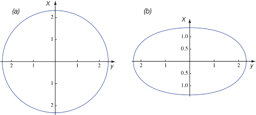
Figure 1: Instantons for different ratios $\gamma={e_{0}E_{0}\xi K_{\rm eff}\over\hbar\omega}{p\pi\over 4}$ of field strength to frequency. (a) for $\gamma 21$, the instanton is almost circular, and (b) for $\gamma=0.2$, the instanton is elongated in time direction.

The domain of integration is bounded by the singularities $\pm y_{0}$ of the integrand and the solution corresponds indeed to an instanton with finite Euclidean action (Fig. 1). The spatial extension of the instanton is

$$L_{x}(\omega,\gamma) = {2v_{\rm eff}\over\omega}\ \arctan{1\over\gamma}$$

$$L_{t}(\omega,\gamma) = {2\over\omega}\ {\rm arcsinh}{1\over\gamma}\ \ .$$ (4.6)

The limiting forms for the static limit $\gamma\to\infty$ and the dynamic limit $\gamma\to 0$ are

$$L_{x}(\omega,\gamma) = v_{\rm eff}\ \left\{\begin{array}[]{cc}{8\hbar v_{\rm eff}\over e_{0}E_{0}\xi K_{\rm eff}p\pi}&\gamma\to\infty\\[14.22636pt] {\pi v_{\rm eff}\over\omega}&\gamma\to 0\end{array}\right.$$ (4.9)

$$L_{t}(\omega,\gamma) = \left\{\begin{array}[]{cc}{8\hbar\over e_{0}E_{0}\xi K_{\rm eff}p\pi}&\gamma\to\infty\\[14.22636pt] {2\ln{2\over\gamma}\over\omega}&\gamma\to 0\end{array}\right.$$ (4.12)

In the static limit, the instanton is circular with an extension inversely proportional to the electric field. In the dynamic limit, the scale for the instanton extension is set by the period of the ac electric field, and it is elongated in time direction by a factor $\ln(2/\gamma)$.

The creation rate of kink antikink pairs is proportional to the negative exponential of the instanton action divided by the space-time volume of an instanton. One finds

$$P(E_{0},\omega) = {\exp{\left[-{2E_{s}\over e_{0}E_{0}\xi K_{\rm eff}p}\;{4\over\pi}\;\gamma\;{\rm F}(\gamma)\right]}\over L_{x}(\omega,\gamma)L_{t}(\omega,\gamma)}$$ (4.13)

$${\rm F}(\gamma) = \int_{0}^{{\rm arsinh}{1\over\gamma}}\!\!\!\!\!\!\!\!\!du\sqrt{1-\gamma^{2}\sinh^{2}u}\ .$$

This result would be changed by a preexponential factor when including the contribution of fluctuations of the instanton shape, of zero modes, and of the Jacobi determinant originating in the transition from an integral over the field $\varphi$ to an integral over the the domain wall position Langer67 ; Kleinert . The dependence of the exponent on $\gamma$ is displayed in Fig. 2. For the static limit with frequencies $\omega\ll e_{0}E_{0}\xi$, $\gamma$ is large and we find

$$\gamma F(\gamma)\to{\pi\over 4}\left[1-{1\over 8\gamma^{2}}+O({1\over\gamma^{4}})\right]\ \ .$$ (4.14)

According to the expansion Eq. (4.14), the first correction of order $\omega^{2}$ reduces the static value of the exponent. Hence, for a fixed field amplitude $E_{0}$, the creation rate increases monotonically with frequency.

In the dynamic limit of large frequencies, one finds

$$\gamma F(\gamma)\ \to\ \gamma\ln\left({4\over e\gamma}\right)\ \ .$$ (4.15)

This result gives rise to an instanton creation rate

$$P(E_{0},\omega)={\omega^{2}\over 2\pi v_{\rm eff}\ln{2\over\gamma}}\left({e_{0}E_{0}K_{\rm eff}\xi p\over\hbar\omega}{e\pi\over 16}\right)^{4E_{s}\over\hbar\omega}\ \ .$$ (4.16)

This instanton creation rate can be interpreted in terms of multi-photon absorption: the optical gap in the system is $2E_{s}$, and hence the smallest integer larger than the ratio $2E_{s}\over\hbar\omega$ determines the number of photons necessary to create one soliton-antisoliton pair. The ratio of electric field strength to photon energy in the brackets agrees exactly with the noninteracting result Eq. (2.4) if one identifies $E_{g}=2E_{s}$, uses the definition of the soliton energy, and considers the fermionic case $p=2$.

The present semiclassical approximation can be expected to work well for $\hbar\omega\ll E_{s}$ when the photon number is large and the electrical field can be treated unquantized. However, it does not reproduce the threshold behavior expected whenever the photon energy is tuned through an integer fraction of the optical gap $2E_{s}$. The specific physics of a Mott insulator as compared to a band insulator is contained in the energy dependent form factor, which for the band insulator is just the density of states. The energy dependence of the form factor is probably contained in fluctuation corrections around the saddle point, which would be interesting to calculate. The main conclusion from the agreement between the semiclassical and the quantum mechanical result is that the dominant electric field dependence for the Mott insulator is similar to that of the band insulator when expressed in suitable effective quantities, which parameterize the interaction strength.

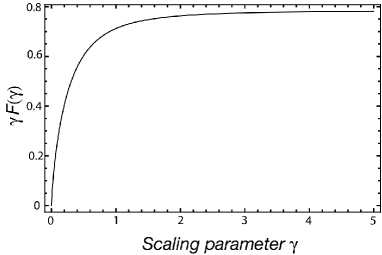
Figure 2: Dependence of the exponent of $P_{E}$ on $\gamma={e_{0}E_{0}\xi K_{\rm eff}\over\hbar\omega}\ {\pi\over 4}$. The exponent grows monotonically with $\gamma$ and saturates for $\gamma\to\infty$.

V Nonlinear Conductivity

The quantum sine-Gordon model is integrable, and in the absence of additional interaction terms or a coupling to a dissipative bath its solitonic excitations have an infinite life time. According to this logic, even an infinitesimally small density of solitons would give rise to an infinite dc conductivity. This conclusion does not sound realistic, and in the following we will discuss the behavior expected from physical systems which are approximately described by this model.

As both kinks and antikinks carry a topological quantum number, they cannot simply decay but only annihilate each other Buttiker86 . Pairwise annihilation gives rise to a decay rate $P_{\rm decay}\sim n_{\rm eq}^{2}$ and hence $n\sim\sqrt{P(E_{0},\omega)}$ in equilibrium. As kinks and antikinks are solitary waves, this annihilation is only possible in the presence of a dissipative bath.

In the dynamic limit with multi-photon absorption, the kink and anti-kink created by the electric field stay close to each other and it seems plausible that they will annihilate quickly such that the nonlinear ac conductivity can be calculated according to Eq. (2.5).

The static limit is more subtle. Maki Maki77 ; Maki78 suggested to calculate the conductivity according to Eq. (2.5) in the dc limit as well, which would imply that every kink and antikink that come close to each other annihilate with certainty. This assumption would only be justified if the coupling to the dissipative bath was strong. If the coupling to the dissipative bath was weak, there would be a finite density of kinks and antikinks, and the conductivity would depend on their mean free path. Under the assumption DaSa05 that the mean free path is of the order of the inter-particle distance, the product of equilibrium density and mean free path would be of order one, and the conductivity would not be exponentially suppressed anymore, a result quite different from the exponential suppression in the case of strong dissipation.

In summary, we have discussed the nonlinear ac conductivity of interacting 1d electron systems in a periodic potential. We found that the dominant physical process in the dynamical limit is multi-photon absorption, and that the result of an instanton calculation is in quantitative agreement with a fully quantum mechanical calculation for noninteracting electrons in the limit of a large number of simultaneously absorbed photons.

Acknowledgments: This paper is dedicated to Thomas Nattermann on the occasion of his 60th birthday. I would like to thank him for generously sharing his deep knowledge about disordered systems with me, and I am indebted to him for collaboration in an early stage of this research. I would like to thank E. Heller and S. Sachdev for interesting discussions, and the Heisenberg program of DFG for support.

References

- (1) T. Giamarchi, Quantum Physics in One Dimension (Oxford Univ. Press, 2003).
- (2) G. Grüner, Density Waves in Solids (Addison-Wesley, New York, 1994).
- (3) H. Kleinert and K. Maki, Phys. Rev. B 19, 6238 (1979).
- (4) D. Controzzi, F.H.L. Essler, and A.M. Tsvelik, Phys. Rev. Lett. 86, 680 (2001).
- (5) T. Giamarchi, Phys. Rev. B 44, 2905 (1991).
- (6) K. Damle and S. Sachdev, Phys. Rev. Letters 95, 187201 (2005).
- (7) K. Maki, Phys. Rev. Lett. 39, 46 (1977).
- (8) K. Maki, Phys. Rev. B 18, 1641 (1978).
- (9) B.S. Wherret, J. Opt. Soc. M. B 1, 67 (1984).
- (10) J,W. Negele and H. Orland,Quantum Many-Particle Systems, Addison-Wesley (1988).
- (11) J. S. Langer, Ann. Phys. (N.Y.) 41, 108 (1967).
- (12) H. Kleinert, Path Integrals in Quantum Mechanics, Statistics and Polymer Physics (World Scientific, Singapore, 1995).
- (13) M. Büttiker, in proceedings of the MIDIT workshop on Structure, Coherence and Chaos in Dynamical Systems, eds. P.L. Christiansen and R.D. Parmentier (Manchester University Press, 1986).
- (14) B. Rosenow and T. Nattermann, Phys. Rev. B 73, 085103 (2006).