Optical Selection of Faint AGN in the COSMOS field

Abstract

We outline a strategy to select faint ($i_{AB}<24.5$) type 1 AGN candidates down to the Seyfert/QSO boundary for spectroscopic targeting in the COSMOS field (Scoville et al., 2007). Our selection process picks candidates by their nonstellar colors in $uBVRizK$ broadband photometry from the Subaru and CFH Telescopes and morphological properties extracted from HST ACS $i$ band data. Although the COSMOS field has been used extensively to survey the faint galaxy population out to $z\sim 6$, AGN optical color selection has not been applied to so faint a level in such a large continuous part of the sky. Hot stars are known to be the dominant contaminant for bright AGN candidate selection at $z<2$, but we anticipate the highest color contamination rate at all redshifts to be from faint starburst and compact galaxies. Morphological selection via the Gini Coefficient separates most potential AGN from these faint blue galaxies. Recent models of the quasar luminosity function (QLF) from Hopkins et al. (2007) are used to estimate quasar surface densities, and a recent study of stellar populations in the COSMOS field (Robin et al., 2007) is applied to infer stellar surface densities and contamination. We use 292 spectroscopically confirmed type 1 broad line AGN and quasar templates to predict AGN colors as a function of redshift, and then contrast those predictions with the colors of known contaminating populations. Since the number of galaxy contaminants cannot be reliably identified with respect to stellar and predicted QLF numbers, the completeness and efficiency of the selection cannot be calculated before gathering confirming spectroscopic observations. Instead we offer an upper limit estimate to selection efficiency (about 50$\%$ for low-z and 20-40$\%$ for int-z and high-z) as well as the completeness and efficiency with respect to an X-Ray point source population (from the COSMOS AGN Survey), in the range 20$\%$ to 50$\%$. The motivation of this study and subsequent spectroscopic follow up is to populate and refine the faint end of the QLF, at both low and high redshifts, where the population of type 1 AGN is presently not well known. The anticipated AGN observations will add to the $\sim$300 already known AGN in the COSMOS field, making COSMOS a densely packed field of quasars to be used to understand supermassive black holes and probe the structure of the intergalactic medium in the intervening volume.

1. INTRODUCTION

Optical colors provide a well-developed, reliable astronomical selection technique for stellar and galaxy populations. The method was first applied to AGN in the 1960’s, based on the inference that quasars often have a larger ultraviolet excess than the hottest stars (Sandage & Wyndham, 1965). Subsequent large-scale surveys have taken up the search for quasars (e.g. Schmidt & Green, 1983; Foltz et al., 1987; Croom et al., 2001; Schneider et al., 2007), causing the known population to grow dramatically. The ongoing search to find new quasars is highly motivated by their use in probing the intergalactic medium (IGM) and understanding the nature of supermassive black holes. To efficiently target and identify new quasars, optical selection techniques have proven to be highly efficient, in some cases mitigating the need for confirming slit spectroscopy (Richards et al., 2002, 2004). Richards et al. (2002) used multi-color imaging from the Sloan Digital Sky Survey (SDSS) to select AGN and quasars down to magnitudes $i_{AB}<21$. In this paper we apply optical selection to the COSMOS field (Scoville et al., 2007), probing the AGN population to much fainter magnitudes ($i_{AB}<24.5$) than any previous large-area survey, and we reveal challenges unique to the fainter AGN population and its contaminants. To properly account for contamination of the AGN candidate pool, we characterize the stellar populations that are dominant at $i_{AB}<21$ and the galaxy population that are more prevalant at fainter magnitudes.

Targeting the AGN population to such a faint level is key to understanding bulk properties of AGN and constraining the faint end of the quasar luminosity function (QLF) at high redshift, which is highly unknown and can vary in up to two orders of magnitude at $i>23$ (e.g. pure luminosity evolution vs. luminosity dependent density evolution most recently presented in Hopkins, Richards, & Hernquist, 2007). With a more complete QLF, astronomers can analyze the nature of low luminosity quasars further $-$ answering important questions about their host galaxies and environments. Such objects are also useful for interpreting the low mass end of the black hole M-$\sigma$ relation, and for probing the IGM. A particular goal of observing faint AGN is to measure the growth rate of lower mass black holes and/or AGN that accrete with lower efficiency. This faint survey brings quasar selection into a new regime of luminosity, placing new observational bounds on theoretical ideas about the nature and evolution of quasars.

Richards et al. (2004) used two 3D multi-color spaces to select QSO candidates in SDSS: $ubri$ $(u-b,b-r,r-i)$ for lower redshift candidates and $briz$ $(b-r,r-i,i-z)$ for candidates with $z>2.5$. The AGN population with $2.5<z<3.0$ is well known to exhibit colors similar to A stars and thus is extremely difficult to isolate via optical means (Richards et al., 2002; Fan, 1999; Richards et al., 2001), justifying a split of the selection algorithm into high and low redshift components. Following the SDSS group, we use a $u-B$ baseline for $z<2.5$ and a combination of $(B-V)$ and $(V-i)$ colors to target AGN with $z>3.0$. The intermediate redshift range ($2.5<z<3.0$) is also targeted and follows similar selection criteria as the high redshift selection, but we expect a much lower object yield in this range due to heavy contamination from faint blue stars. Unlike the SDSS group, we do not anticipate recovering the AGN population with equal efficiencies across all redshifts. Our goal is to push AGN selection to fainter magnitudes while maintaining reasonable efficiency ($>20\%$) and completeness ($>30\%$). Unique to our survey is the use of morphological information (via the ACS images) to separate the marginally resolved AGN galaxies and unresolved stars (only prominent in number at the brighter magnitudes) from more clearly resolved galaxies.

Since the goal of this study is to realistically constrain the faint AGN population, we hope to target a significant portion of our AGN candidates during future spectroscopic ovservations, anticipating anywhere from 30-50 AGN yeild per night by observing $\sim$100 candidates, as well as gaining important information from the spectroscopic details of contaminating galaxies. Already, $\sim$160 candidates, chosen by the methodology of this paper, have been observed at Magellan IMACS and LDSS3 as of May 2007 and more observations are planned. By building up significant statistics on low-luminosity AGN in COSMOS, such a large swath of the sky, we are in a unique positions to improve what is known about the AGN population with meaningful statistics at the limit of current observations.

This paper thoroughly discusses the development of a reliable optical AGN selection algorithm, current knowledge of the QLF, and estimates of our algorithm’s efficiency and completeness; observations and further development of the QLF will be discussed in a follow-up paper. The catalogs and data used in the development of a selection algorithm are discussed in §2. The colors and nature of the contaminating populations are discussed in §3, while our method of morphological selection is given in §4. The specifics of the AGN selection are detailed in §5. In §6 we discuss the current picture of the QLF, predict number counts of contaminating populations, and discuss estimates to the efficiency of our methodology. We use a standard cosmology with $\Omega_{M}=0.3$, $\Omega_{\Lambda}=0.7$, and $H_{0}=70$ km s^-1Mpc^-1 (e.g. Spergel et al., 2003) and luminosity distances computed according to Hogg (1999).

2. CATALOGS AND TRAINING DATA

AGN candidates were selected from the overlap of two catalogs: the COSMOS photometric catalog (hereafter CPC) from Capak et al. (2007) and the COSMOS HST Morphology Catalog (CMC) from Abraham et al. (2004, 2007). The former contains photometric information in uBVrizK broadband filters and photometric redshifts for 3,234,836 objects in the extended 3.5 square degree Subaru optical field, and 2,326,609 objects in the central 1.7 square degrees covered by Hubble ACS imaging. The central 1.7 square degrees is fully imaged with the F814W ACS filter and the resulting catalog is 95$\%$ complete down to $i_{ACS}=26.0$. The Morphological Catalog (CMC) includes detailed 2D morphology for 195,706 objects restricted by $18.0<i_{ACS}<24.5$, which is $\sim$80$\%$ of all CPC objects within the same magnitude limits. For a plot of the differential number counts, see Figure 1. For reasons elaborated on later (see §3.3) we do not choose to present a purely color dependent algorithm to select AGN candidate objects excluded from the CMC (but part of the CPC), due mainly to heavy galaxy contamination and large increase in photometric errors.

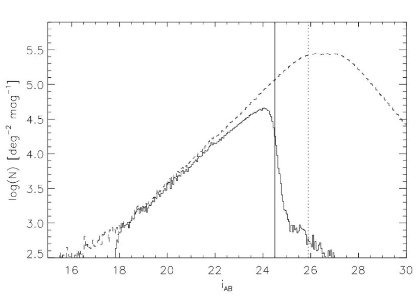
Figure 1.— Differential distribution of $i_{AB}$ apparent magnitude (in a bin size of 0.05 mag) for all objects in the COSMOS photometric (dashed) and morphological (solid) catalogs. The larger COSMOS Photometric Catalog (CPC) contains over 2 million objects in the central $\sim$2 square degrees ($\sim$ 90 $\%$ of which have $i_{AB}>24.5$) and becomes incomplete fainter than $i_{AB}=25.9$ (dotted line). The morphological catalog (the subset of the CPC defining our candidate pool) contains about 195,000 objects, constrained approximately by $18<i_{AB}<24.5$ and exactly by $18<i_{ACS}<24.5$. As discussed in the text, $i_{auto}$ is used throughout the paper to denote $i_{AB}$ because it most accurately represents the full integrated flux in the standard AB-system $i$ band. Within the magnitude range of interest ($18<i_{AB}<24.5$), about 80$\%$ of all CPC objects are also contained in the COSMOS Morphological Catalog (CMC); the discrepancy lies largely between magnitudes 23.5 and 24.5.

In addition to the selection catalogs, we consider a “training set” of known AGN in the COSMOS field with confirming spectroscopy (Trump et al., 2007). To model the complex nature of AGN selection, we use the AGN training set, along with four type 1 AGN color templates adapted from SEDs presented by Budavári et al. (2001). A recent analysis of the COSMOS stellar population (Robin et al., 2007) is used to estimate contamination levels from stars after establishing the algorithm. A list of 1073 X-Ray point sources (hereafter XRPS) with no spectroscopy are used to test algorithm efficiency after the method design has been explained.

2.1. COSMOS Photometric Catalog

Data are drawn from the 3 Jan 2006 data release of the Cosmic Evolution Survey (COSMOS) $\sim$2 square degree equatorial field imaged with large ground-based telescopes (Subaru, VLA, ESO-VLT, UKIRT, NOAO, CFHT) and space-based observatories (Hubble, Spitzer, Galex, XMM, Chandra). The latest release of the photometry catalog (CPC) includes detections for over 3 million objects in the Subaru $i+$ band filter in an extended 3.5 square degree field (the offset to SDSS $i$ is +0.3 magnitudes), and magnitudes in CFH $u*,i*$ (hereinafter denoted $u$, $i_{c}$), Subaru $Bj,Vj,r+,i+,z+$ (denoted $BVriz$), Kitt Peak CTIO $Ks$, narrow-band Subaru $NB816$, and $F814W$ HST ACS band ($i_{ACS}$). The CPC’s main use by the COSMOS collaboration has been to survey the galaxy population, of which over 2 million galaxies have been detected out to $z\sim 3$ (Scoville et al., 2007; Capak et al., 2007). Imaging in F814W with Hubble ACS provides sufficiently deep data for reliable morphological classification down to $i_{ACS}>24.5$, described more fully in §2.2.

Photometric redshifts are estimated via two methods$-$the COSMOS team code (Mobasher et al., 2006), and the Baysian Photometric Redshift (BPZ) code (Benítez, 1999). The dispersion in photometric redshifts is comparable and small in either case ($\sigma(z)/z\sim 0.04$), but the Mobasher code measures reddening and does a better job of breaking redshift degeneracies. Although the photometric redshifts are effective for Hubble-typing galaxies, they are clearly inappropriate for our AGN candidates, which have complex, multi-component spectra not easily characterized by SED fitting based on stellar populations. Neither photometric redshift code uses AGN templates. We will use the photometric redshifts to quantify galaxy color properties and understand the contamination rates as a function of redshift, for which both methods (Mobasher and BPZ) are reliable and produce similar results.

The photometric catalog quotes a detection band magnitude, $i_{auto}$, which defaults to Subaru magnitudes in $i+$ except in the case where the source is saturated or missing in the Subaru image and CFHT $i*$ is used instead. The subscript $auto$ refers to the SExtractor AUTO aperture used to calculate magnitudes inside an adjustable, elliptical isophote (Bertin & Arnouts, 1996). CFHT magnitudes dominate $i_{auto}<20.1$ (these are saturated sources in Subaru photometry), and constitute a smaller population of objects at fainter magnitudes, out to 24. For objects with photometry in both bands, the CFHT and Subaru magnitudes are consistent out to $i=26.0$, fainter than the AGN candidates which are limited by the depth of the morphological catalog ($i_{auto}\sim 24.5$). With this understanding, we will not distinguish between them and will operate in terms of apparent magnitude $i_{AB}$, which throughout this paper will refer to $i_{auto}$. All other magnitudes in the catalog are calculated using a SExtractor fixed aperture with $3\arcsec$ diameter and are only used when discussing colors.

Table 1Limiting and Completeness Magnitudes for Cosmos Photometry.

BAND	LIMITING	COMPLETENESS
$U_{C}$	26.3$\pm$0.4	27.1$\pm$0.1
$B_{S}$	25.6$\pm$0.4	26.7$\pm$0.2
$V_{S}$	25.6$\pm$0.5	26.6$\pm$0.2
$R_{S}$	25.7$\pm$0.4	26.2$\pm$0.1
$I_{S}$	24.6$\pm$0.5	25.9$\pm$0.2
$I_{C}$	23.1$\pm$0.4	25.2$\pm$0.1
$Z_{S}$	23.6$\pm$0.6	25.4$\pm$0.2
$K_{K}$	20.1$\pm$0.3	22.9$\pm$0.1

Note. — The limiting magnitude is defined by the faintest magnitude (M) of which $\sigma_{M}/M<$10$\%$. The completeness magnitude is the magnitude at which the given band is 95$\%$ complete. The ’C’ subscript corresponds to CFHT photometry, ’S’ corresponds to Subaru, and ’K’ corresponds to Kitt Peak CTIO.

Since optical AGN have an intrinsic spread in their spectral energy distributions (SEDs), the difficulty in selecting candidates is aggravated by photometric errors. For each band that we use during object selection, we quote two characteristic limiting magnitudes: the first is the magnitude at which the error is 10$\%$, and the second is the 95$\%$ limit of catalog completeness. Table 1 shows these magnitudes for each filter. Although the deepest band in the catalog is $B$, and the other bands progressively become shallower at redder wavelengths, $i+$ is chosen as the detection band image because it does not bias against higher redshift objects (except at z$>$5), is not effected sustantially by reddening, is the deepest red band, and is typically used as the detection band for large optical surveys. A $\chi^{2}$ band (a coaddition of $i$ band, $r$ band and $B$ band; see Capak et al., 2007) has increased sensitivity and pan-chromatic advantage and was also considered as a detection band; however, the $i+$ band gives much better resolution needed for high quality photometric calculations.

2.2. COSMOS Morphological Catalog

The COSMOS HST morphological catalog (CMC), generated by Bob Abraham at the University of Toronto (Abraham et al., 2004, 2007), uses single filter ACS imaging to extract 2D morphology classification down to $i_{ACS}<24.5$. The CMC is primarily designed for use in studying the morphological properties of galaxies in the COSMOS field, using 2D parametric and non-parametric measures. In the special version fo the CMC used in this project, morphologies were calculated down to a level too faint for reliable galaxy work, but were enabled by the fact that AGN are generally described by a point source surrounded by a fainter host galaxy. The catalog is not taken to fainter levels because the robustness for even basic morphological calculations deteriorates. The CMC includes ACS magnitudes (total $AUTO$ magnitude), orientation, ellipticity, mean surface brightness, central surface brightness, half light radius, signal to noise ratio, concentration index, and the Gini coefficient (among other parameters not used in this study). Since there is a significant color correction applied between F814W and $i_{AB}$, there is not a clean cutoff at $i=24.5$ for CMC sources in Figure 1. Spurious sources from both ground based and ACS data, especially in the wings of bright sources, causes the tail of few objects out to magnitude $i=26$ which should normally be included in the $18<i<24.5$ range.

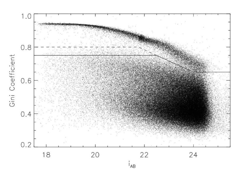
Figure 2.— The behavior of the Gini coefficient ($G$) applied to the COSMOS/ACS i-band mosaic as a function of magnitude. The overall decrease in Gini with magnitude is largely due to observation bias, i.e. fainter sources are found to be more extended since there is less contrast with the image background. Altering the original Gini calculation described by Abraham et al. (2003) algorithm (so as $not$ to use adjustable quasi-Petrosian radii) gives cleaner separation between unresolved sources (across the top), and resolved, extended sources (the bulk of the objects with low $G$). Gini is therefore useful to reject extended galaxies and retain unresolved or marginally resolved stars and AGN. The solid line indicates the $G$ selection criterion adopted later in the paper for low redshift AGN (with candidates chosen to lie above the line), while the dashed line indicates the more conservative boundary used for intermediate and high redshift AGN selection (see §4, §5.1, and §5.2).

The Gini coefficient, hereinafter denoted $G$, is a non-parametric measure of concentration ($0<G<1$, with $G=1$ is a point source with all the flux in one pixel, and $G=0$ is uniformly extended with no discernable center) which doesn’t assume a central pixel or a PSF. The advantage of its use is that it can morphologically characterize galaxies of arbitrary shape and does not require a well-defined nucleus center, which is a more general treatment of PSF classification of stars and galaxies, and includes a wider scope of irregularly or assymetrically shaped objects. For a more detailed treatment and definition of Gini, as well as a description of the term’s origin in economics (Gini, 1912), see Abraham et al. (2003). In its original context (Abraham et al., 2004), Gini is calculated from pixels lying within a set of quasi-Petrosian radii (unique to each object), giving the best 2D morphological analysis needed for galaxy evolution studies. At faint magnitudes ($i_{AB}>24.5$), this approach to calculating Gini breaks down, and compact objects have much lower $G$ than their bright counterparts due to an inclusion of background noise within a more extended Petrosian radius. Since this study requires a clean separation of resolved and unresolved sources, we have altered the Gini computation so that the Petrosian radius is not adjusted from object to object $-$ this makes the decrease in $G$ with fainter magnitude not as severe. The behavior of $G$ with magnitude may be seen in Figure 2. The strip along the top corresponds to unresolved sources (stars, compact AGN) while the large population with low $G$ corresponds to galaxies. Clearly, Gini is most useful to distinguish well-resolved galaxies from unresolved or partially resolved AGN galaxies.

2.3. AGN Training Data

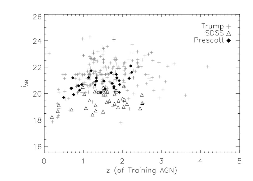
Figure 3.— The type 1 AGN training data’s magnitude as a function of spectroscopic redshift. All data points are in the set of 268 type 1 AGN with color and morphology information (as described in Table 2), and the different symbols represent the three parent data sets: COSMOS AGN survey (Trump et al., 2007), SDSS overlap with the COSMOS field (Richards et al., 2005), and additional spectroscopic follow up of SDSS sources on MMT (Prescott et al., 2006).

Table 2AGN Training Data

	Trump	SDSS	Prescott	TOTAL	USE
(1)	(2)	(3)	(4)	(5)	(6)
All Objects	1334	86	94	N/A	N/A
Unique Objects	1334	75	38	1450	Color on all types of AGN
Type 1 AGN	200	51	38	292	Color on Type 1 AGN
AGN in CMC	1334	41	31	1406	Color and Morph on all types of AGN
Type 1 AGN in CMC	200	37	31	268	Color and Morph on Type 1 AGN

Note. — The AGN Training Data is broken down by source catalog (Trump et al., 2007; Richards et al., 2002; Prescott et al., 2006), and by type (all AGN, type 1 AGN, AGN in CMC and type 1 AGN in CMC). Column (1) describes the type of AGN, column (2) represents objects from the COSMOS AGN Survey (Trump et al., 2007), column (3) represents objects observed by SDSS (Richards et al., 2002, 2005) with confirming spectroscopy, and column (4) represents objects observed by Prescott et al. (2006). The total number of AGN of each type are given in column (5) and their use in our analysis is given in column (6), e.g. the most useful set has both color and morphological information for type 1 AGN and contains 268 objects (the redshift magnitude distribution of these objects is seen in Figure 3).

Table 2 gives details on the AGN training data, the different sets of data they originate from, and the number counts of type 1 AGN, AGN included in the CMC and type 1 AGN included in the CMC. Since the training data sources overlap, the reader should refer to Table 2 for a breakdown of training data sources throughout this subsection. Figure 3 shows magnitude versus redshift for 268 training set AGN (those training AGN for which we have both color and morphology information$-$see 2). With 1450 total spectroscopically observed AGN targets in the COSMOS field, 292 of which are type 1 AGN, we are able to infer colors and morphology as a function of redshift to characterize and calibrate the AGN candidate population. The AGN training data come from four sources: an X-Ray or Radio-selection from the COSMOS spectroscopic AGN survey (Trump et al., 2007), the SDSS optical selection with confirming spectroscopy overlaping the COSMOS field (Richards et al., 2002), and spectroscopically confirmed SDSS optical targets from observations on MMT/Hectospec (Prescott et al., 2006). The observation details on each training data set are given in the following paragraphs. Since the training data sets do overlap, each set is described by the number of unique objects that were not included in previously described training data sets (starting with data from Trump et al., 2007, see Table 2 row 2). We do not use type 2 narrow line AGN in this paper since their optical colors have larger variations due to lower emission flux and obscuration. We anticipate that the candidate objects will mostly be type 1 AGN since at these magnitudes ($i\sim 24$) we need strong, broad emission features and a non-thermal continuum for identification.

The X-Ray/Radio selected sources (limited by $i<23$) come from the first spectroscopic observations of the COSMOS AGN Survey (Trump et al., 2007) using the Inamori Magellan Areal Camera $\&$ Spectrograph (IMACS, Bigelow et al., 1998) on the Magellan (Baade) Telescope. The first year of observations yielded 284 AGN that were given spectroscopic redshifts, 115 of which were originally radio sources and 169 were X-Ray sources (Schinnerer et al., 2007; Brusa et al., 2007). In a second round of observations, 1050 more AGN were spectroscopically confirmed in observations. Type 1 AGN are likely 90$\%$ complete to $i_{AB}<23$. The survey had 72$\%$ targeting yield (the percentage of candidates that are actually AGN) down to $i_{AB}=24$, and a much better yield, $>90$$\%$, for $i_{AB}<22$. A small subset of the observed targets was difficult to classify, but the majority was a variety of type 1 and type 2 AGN. All together, 1334 AGN were spectroscopically observed, 200 of which are type 1 AGN included in the CMC (see Table 2). The intrinsic selection bias between X-Ray/Radio selected objects and optically selected objects is valuable to investigate; while working at much fainter magnitudes than the faintest SDSS optically-selected QSOs ($i=21$), we expect to incorporate the same optical selection biases. Including the X-Ray/Radio objects gives a relatively unbiased or independent sample of the optical properties of the true AGN population, takes the training set to fainter magnitudes ($i=23$) than their optically selected counterparts, and may include more extended well-resolved AGN galaxies which are rejected for optical selection.

The SDSS sample (limited by $i<21$) comes from the overlap region of SDSS on the COSMOS field (from SDSS DR1), originally targeted and selected either optically or as X-Ray sources (see Richards et al., 2002, for selection details). Of the 86 spectroscopically targeted objects (75 unique objects), 51 are type 1 broad line AGN. These sources are primarily well resolved and bright ($i<21$). An additional 119 objects were optically selected as QSOs (Richards et al., 2002, 2004) with high confidence (90$\%$), but only 3 of these objects do not overlap with all other spectroscopic data so were not included in analysis (including observations from Prescott et al., 2006, which are described in the following paragraph).

There are 94 spectroscopically confirmed quasars (38 unique objects) in our training set observed with the MMT 6.5 m telescope and the Hectospec multiobject spectrograph (Prescott et al., 2006). The original 336 targets were marked with quasar flags drawn from the SDSS DR1 catalog, described by the previously discussed SDSS multicolor quasar selection algorithm. Eighty out of the 94 quasars did not appear in previous follow-up confirmation studies. The quasars span a range of magnitudes $18.3<g<22.5$ and redshifts $0.2<z<2.3$, and the results from this study support the lower limit of the quasar surface density from SDSS color selection of 102 AGN per square degree down to $g=22.5$ over the entire COSMOS field.

2.4. Narrow Emission Line Galaxies

Additional observations on MMT/Hectospec from Prescott et al. (2006) give 168 narrow emission line galaxies (NELGs) in the COSMOS field$-$objects that were originally tagged as probable AGN from SDSS color selection but were found to be NELGs in spectroscopic follow-up. Since these objects share the same colors as AGN, this set acts as a control for blue galaxies used to understand galaxy morphology and necessary components of the morphological selection design (see §4). They span redshifts $0.2<z<2.3$ and magnitudes $18<i<22.5$. These NELGs are used exclusively to understand contaminants and probe selection efficiency.

2.5. X-Ray Sources

From an original set of 1865 X-Ray point sources (XRPS) in the COSMOS field Brusa et al. (2006, 2007); Hasinger et al. (2006, 2007); Cappelluti et al. (2007), the set is narrowed down to 1073 objects who have 98$\%$ confidence that their optical identification is secure, and are contained in the CMC (Brusa et al., 2007). They are used in this paper as a test set and are treated separately from the spectroscopically confirmed training set from §2.3. The XRPS were not spectroscopically targeted by Trump et al. (2007) either because they were too faint for IMACS targeting, they were not allocated a slit during observations, or they lay outside regions of the 2-degree field targeted with IMACS to date. This sample is less useful in formulating the algorithm designs despite its large numbers. In terms of both colors and Gini, the optical counterparts to optically faint XRPS show a wide range of properties and many are low luminosity, low redshift Seyfert galaxies. Select spectroscopy reveals that 50$\%$ are Type 1, 33$\%$ are Narrow Line Type 2, and 17$\%$ are ellipticals. We return to this sample at the analysis stage to assess the selection efficiency and completeness, and we use it roughly in the discussion of the high redshift selection procedure (see §5.2).

2.6. AGN Templates

The training set described in §2.3 gives mean AGN colors out to $z_{spec}\sim 3$. Since we intend to target AGN out to $z\sim 6$, templates developed by Budavári et al. (2001) are used to infer colors at higher redshift. Budavári et al. developed four type 1 AGN templates. Rather than characterizing physical differences between AGN, these portray four optimal/empirical fits to observed type 1 SEDs. We compare the template color predictions with the training data and use the best fit template to predict AGN colors at higher redshift (which will be shown later in Figure 6), where the training data run out. Although there is significant variation in color between templates (up to $\Delta$m $\sim 0.5$), there is also intrinsic spread in AGN color about the mean (as seen by the training set objects, $\sigma\ \sim\ 0.3$ mags), so the particular choice of template is not critical. This observed color variance is a function of magnitude and thus also of redshift, but we assume for simplicity that the spread about the best fit template is $\sigma=\Delta m=0.3$. The use of the AGN color templates will later be depicted graphically in Figures 6 (AGN color with redshift), 7 (galaxy colors with redshift), 12 (template track in $V-i$ vs. Gini), and 13 (the 2D color selection for $z>2.5$ candidates with template tracks overplotted).

2.7. Stellar Surface Density

A recent study of the stellar populations in the COSMOS field done by Robin et al. (2007) uses HST morphology coupled with detailed stellar SED fits to identify stars with 90$\%$ completeness at $i=27.0$. Their estimate (later described as the ’strict’ SED fit) of the COSMOS stellar population agrees well with traditional models and observations of star counts (Chen et al., 2001; York et al., 2000; Chen et al., 1999; Bahcall & Soneira, 1981; Reid & Majewski, 1993). This sample is useful when assessing the selection algorithms’ completeness and efficiency relative to contaminating stars. Their methodology identifies point sources via magnitude and central surface brightness (the $MU\_MAX$ SExtractor parameter). We support the “strict” SED method outlined in their paper (Robin et al., 2007) since the number counts procured by the SED method agree with our more crude estimation of stellar counts identified solely through an identical morphological point-source identification. Robin’s “loose” SED restriction on the quality of the SED fits results in much greater stellar density counts (by a factor of ten at the faint end) and largely disagree with other observations of star counts from the literature. They include the “loose” SED fit data to their study to demonstrate the difficulties of star/galaxy separation and gradient of possible separation methods. Our point-source identification is done in three ways: (1) magnitude and central surface brightness (denoted CSB), (2) magnitude and half-light radius (denoted RHO), and (3) the intersection of those two methods. As seen in Figure 4, all of these methods produce roughly the same stellar surface densities as the “strict” stellar SED fitting method. While there is the possibility that many of the AGN we are trying to target might be mislabeled as stars in this set, the number counts of stars substantially outweighs the number of possibly selected AGN. Since we do not use this stellar set to precisely predict colors apart from AGN (save the rough preliminary estimates shown in Figure 5) and instead use it to predict stellar number counts, the inclusion of AGN is countably negligible. In §6, we pass this population (identified in both the CMC and CPC) through our AGN selection filters to determine the level of stellar contamination as a function of magnitude, which leads to estimates of efficiency and completeness.

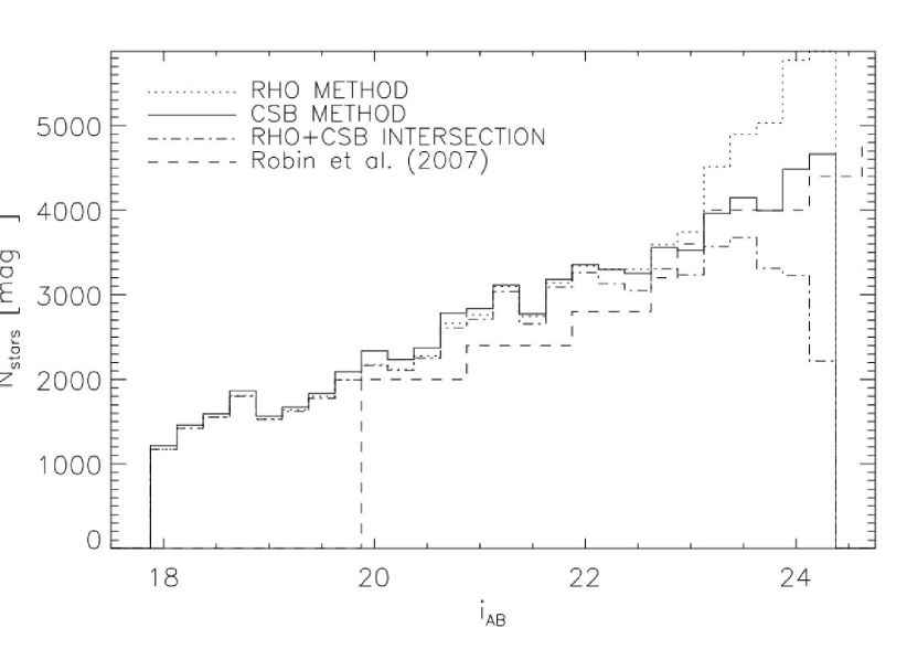
Figure 4.— The results of stellar selection using central surface brightness (CSB) and half-light radius (RHO), the intersection of those two techniques, and comparing the stellar surface densities to those of the Robin et al. (2007). All three methodologies agree roughly with Robin’s “strict” SED method shown here (the CSB selection working best) while Robin’s “loose” SED fit method is an order of magnitude higher at the faint end, which we assert cannot be representative of the true stellar surface density. While the Robin et al. (2007) method presumably isolates stars, such objects are not excluded from the set of candidate AGN since their prior identification as stars cannot be certain.

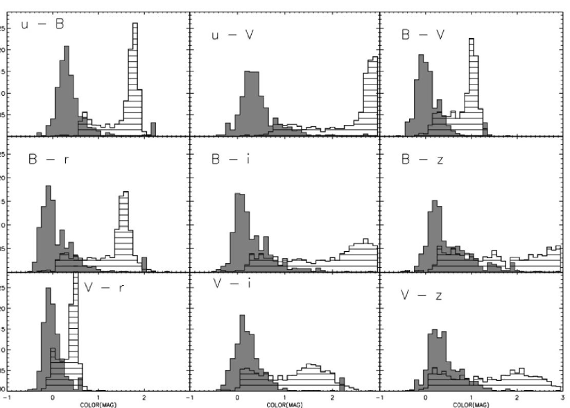
Figure 5.— Colors of the training set of 292 AGN (solid gray) and 1791 bright stars in the COSMOS field as identified by Robin et al. (2007) (lined). The distributions are normalized to equal numbers to more easily show relative colors. To select $z<2.5$ objects with the lowest stellar contamination rate, a short blue baseline is used (i.e. $u-B$, $u-V$), not only because of the clear separation but also because these are the deepest bands, optimal for lower luminosity AGN. As is discussed in the selection portion of the paper (§5), the division between AGN candidates and stars is taken at $u-B$ = 0.67.

3. COLOR SELECTION

The use of colors here differs from previous practice (e.g. Richards et al., 2002, 2004) in that efficient selection is possible without incorporating every available band into the criteria. Since quasars exhibit power law continua with a strong UV excess, the choice of $u-B$ to select lower redshift objects is well motivated and historically successful (Sandage & Wyndham, 1965; Koo & Kron, 1982; Warren et al., 1991; Hewett et al., 1995; Hall et al., 1996; Croom et al., 2001; Richards et al., 2002). Incorporating the additional information from redder baselines for low redshift, like $B-V$ and $V-r$, does not improve selection efficiency on the training set, as discussed in §5.1. In contrast, intermediate and high redshift selection requires a more sophisticated approach since no single color is ineffective in distinguishing stars and AGN. The optimum 2-color choice for both intermediate and high redshift selection, $B-V$ and $V-i$, considers both the depth of the bluer bands, and the need to look towards the red bands for high-z candidate objects. By selecting subsets of the catalog that represent stellar and galaxy populations and investigating their colors as a function of apparent magnitude, we conclude that the color selection method will be uniform across the entire magnitude range ($18.0<i_{AB}<24.5$).

3.1. AGN Colors with Redshift

The colors of AGN as a function of redshift are illustrated in Figure 6 for our three primary colors, $u-B$, $B-V$ and $V-i$. However the spread of AGN color (from the 292 type 1 AGN) is consistently large in each color ($\Delta$$m\sim 0.3$). Our low redshift object selection declines rapidly in efficiency at $z\sim 2.4$ where the mean $u-B$ becomes significantly redder and crosses the stellar locus as Ly$\alpha$ emission enters the B band. This is the natural boundary of the low redshift selection. A similar reddening happens at slightly higher redshift in $B-V$; however, this band adds selection power because AGN are redder than the contaminating stars for $z>4$. An even redder baseline, $V-i$, shows a much flatter shape as a function of redshift, and is used together with $B-V$ to optimize selection of high redshift, faint candidate AGN, as described in §5.2.

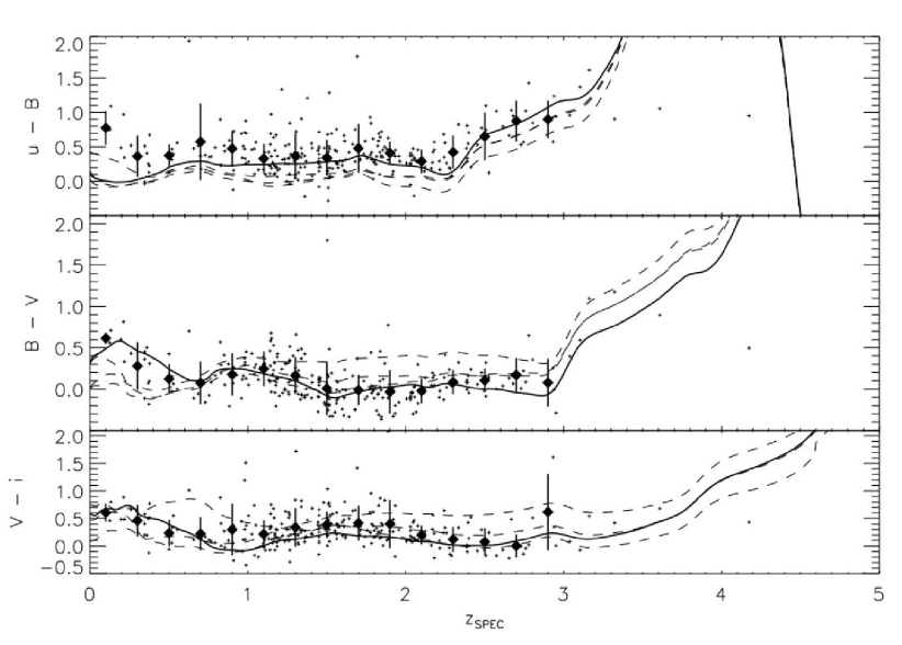
Figure 6.— AGN colors as a function of redshift. The 292 type 1 training AGN (selected as defined in the text) are small dots, the diamonds represent the mean of the training colors (and a 1$\sigma$ spread) taken in $\Delta$z = 0.2 redshift bins, and the four lines (3 dashed, 1 solid) are the colors predicted from templates. The solid line is the preferred template, as judged by deviation from the mean training colors. Although the training data only extend to $z=3$, template colors can be used to anticipate high redshift AGN colors. These colors rise for $z>3$ as Lyman-$\alpha$ emission and then the Lyman limit passes from u-band to B and the redder bands. A sharp drop occurs in the predicted $u-B$ color at $z\sim 4.5$ as the Lyman limit passes through the B band, rendering near zero flux in both bands.

The training data agree broadly with the four type 1 templates from Budavári et al. (2001) up to the limit of the data around $z=3$, with the exception of the lowest redshifts in $u-B$, where the AGN are redder than all templates. Figure 6 shows as a solid curve the template that best fits the data, which is used for the predictions of AGN colors at $z>3$. Colors at high redshift are inevitably uncertain. At $z\sim 4.5$, the Lyman limit passes through both u and B bands, rendering nearly zero flux in both filters and causing a sharp drop in predicted $u-B$. The usefulness of each color will become more apparent as we consider the contaminating populations.

3.2. Colors of Stellar Contaminants

At magnitudes brighter than 21, stars are the primary contaminant in AGN selection. Our goal is to classify and choose AGN candidates at all ranges of magnitudes ($18.0<i<24.5$), so it is important to quantify stellar colors since stars cannot be distinguished from compact AGN morphologically, and they consist of about 10$\%$ of the catalog even at the faintest levels.

We characterize the contaminating stellar population at bright magnitudes ($i<19$) to eliminate effects from large photometric errors at faint magnitudes. This population, a subset of the stars described in §2.7, can be used in lieu of the entire star population since we have confirmed empirically that the stellar colors do not change or redden inherently as a function of apparent magnitude (for this fixed galactic latitude and assuming low photometric error). This sample has 1791 stars$-$sufficient to understand color distributions. Figure 5 shows colors of AGN and stars, indicating which colors are useful in distinguishing the populations. This reaffirms $u-B$ as the best discriminator between the two populations at redshift $z\leq 2.5$.

3.3. Colors of Galaxy Contaminants

Fainter than $i\sim 21$ (where our selection focuses), the overwhelming majority of objects are galaxies, and therefore galaxies are the major of contaminant of the AGN population. As described by Scoville et al. (2007) and Mobasher et al. (2006), all sources are fit by Hubble type galaxy SEDs, yielding photometric redshifts in the range $0<z<3$. For the sources with the most reliable photometric redshifts (given by $\chi^{2}<25$, only the best $\sim 13\%$ of the CPC), we investigate color as a function of redshift for the primary contaminants: starburst and spiral galaxies. Although elliptical galaxies can theoretically be confused with high-z AGN because they are compact and red, they are statistically rare and only present in the catalog in significant numbers at the most recent epochs, $z<0.4$. Since AGN in this low redshift range are much bluer than the red, compact ellipticals, we can easily reject ellipticals. It is worth noting that COSMOS observations of galaxy color are available for $0<z<3$, but photometric redshifts are not reliable at higher redshifts.

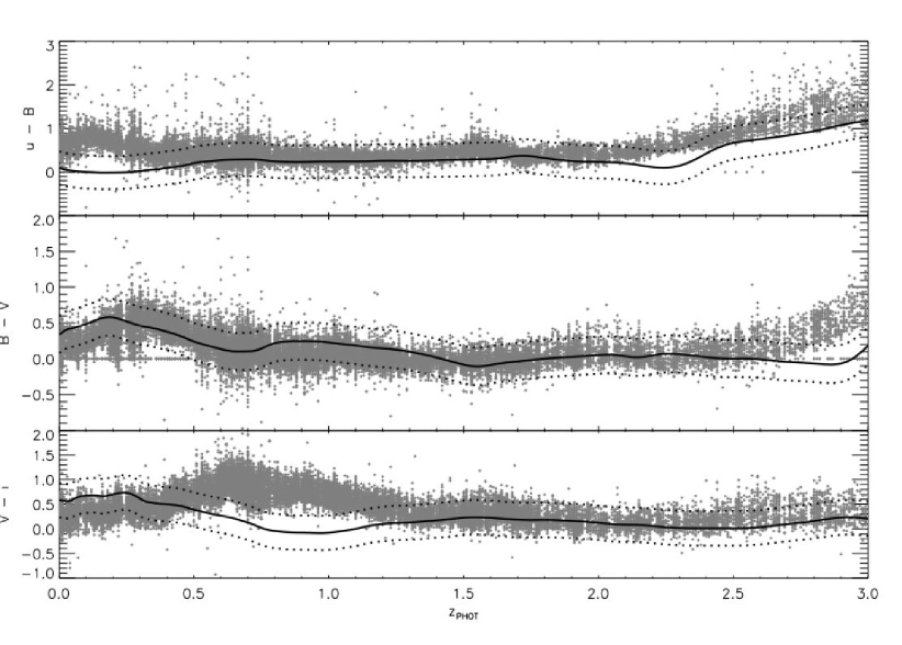
Figure 7.— The primary color contaminant for the AGN sample are galaxies with young stellar populations: spirals and starbursts. Objects identified as starbursts (COSMOS catalog notation $T_{phot}$ = 5,6) with good confidence ($\chi^{2}<25$) are shown here in $(u-B)$,$(B-V)$, and $(V-i)$ colors as a function of photometric redshifts, compared to the preferred AGN templates from Figure 6 (solid lines with $1\sigma$ range as dotted lines). Spiral galaxy colors are similar at all redshifts. While there are small windows in redshift where the galaxy colors differ from AGN, there is no way to incorporate this into the selction method since there is no prior redshift indication for our candidates.

Figure 7 shows color $u-B$ as a function of photometric redshift (for objects with $\chi^{2}<25$ in the CPC) for starburst galaxies. Spirals exhibit very similar colors with a slighly higher overall variance. To clearly understand the level of contamination with AGN, we have overlaid the best fit AGN template from Figure 6 with its 90$\%$ confidence interval illustrated by the dotted lines (determined previously in §2.6). Unlike the case for the stellar population, there is little difference in color between AGN and starburst galaxies, which is why we add morphological information as the basis of our low redshift selection technique.

We considered the possibility of targeting very faint ($24.5<i<25.9$) AGN candidates (which due to their faint magnitudes are not included in the CMC) using only color information, assuming that the only statistically significant contaminants are faint blue galaxies. This could work only if AGN colors and galaxy colors varied over $0<z<3$ or if two significantly distinct colors (one of them being $u-B$ to target UV excess at low redshift) showed strong separation between these two populations over smaller but identical spans in redshift. Unfortunately neither of these criteria is satisfied, so color selection is not effective at extremely faint magnitudes. We also attempted to target $i>24.5$ objects using the image $FWHM$ from ground-based data, a less sensitive morphological discriminator than Gini calculated using ACS data. However, most faint objects regardless of their classification by SED as stars, galaxies, or AGN have unresolved profiles with $2.0\arcsec<FWHM<2.5\arcsec$. Since it is clear that the HST morphology is needed to target faint candidates, we limit our selection to targets included in the CMC.

4. MORPHOLOGICAL SELECTION

The goal of using morphological selection is to distinguish the predominantly compact, centrally concentrated AGN from the typically more extended galaxies that dominate the faint reaches of the catalog. As described in §2.2, the Gini coefficient is a non-parametric measure of source concentration, independent of potential asymmetries or of the nature of the radial profile. The Gini coefficient presents particularly strong leverage when targeting the slightly resolved AGN galaxies; other methods (e.g. see Abraham et al., 2003, for concentration index) require an assumed central pixel and PSF model while Gini simply distinguishes the brightest pixels from the much fainter extended component and is insensitive to the spatial arrangement of those pixels.

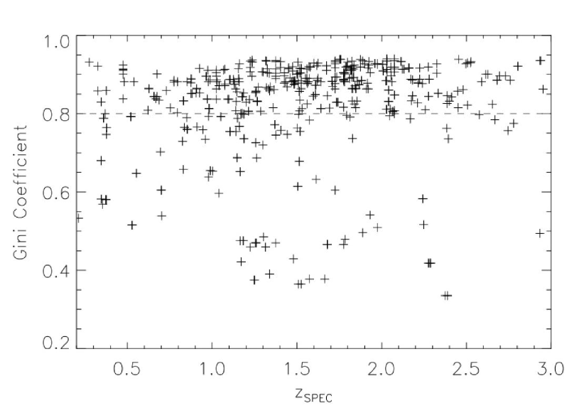
Figure 8.— Gini Coefficient as a function of redshift for 268 type 1 AGN (with both morphological and color data) shows that the majority of the training set of AGN, particularly at $z>2.0$, have $G>0.8$, indicating essentially unresolved sources. At lower redshift, a large spread in $G$ motivates a lower constraint on $G$ (also a function of magnitude as shown in Figure 2). Significant color contamination by galaxies makes it impossible to recover any well-resolved AGN galaxies with $G<0.65$.

Figure 8 shows the Gini coefficient as a function of redshift for the 268 type 1 AGN that had confirming spectroscopy in the training set. While some low and moderate redshift AGN are well resolved with $0.3<G<0.7$, the majority ($\sim$70$\%$), particularly for $z>1$, are unresolved with $G>0.8$. Since we have chosen to divide our selection algorithm into low, intermediate and high redshifts, we will use different Gini criteria for the two regimes, following the behavior illustrated in Figure 8. Although it is difficult to use models to predict the behavior of Gini with redshift (due to cosmic evolution and the wide range of host galaxy properties), we already know that AGn are largely unresolved for $z>1.5$. The Gini coefficient will naturally increase with redshift due to the diminishing contribution from the host galaxy, particularly in the $i$ band; the 4000 Å break passes the $i$ band at $z\sim 1$.

Figure 2 showed that Gini effectively separates unresolved stars from galaxies. Also with the added information from Figure 8 that most AGN are unresolved or marginally resolved in terms of Gini, Figure 2 shows the cuts made in Gini and magnitude to select AGN. At faint magnitudes, unresolved sources have lower $G$ (the right end of the arc), so to include them we drop the lower limit of $G$ to 0.65 as shown. At brighter magnitudes, we allow more extended or resolved sources in our low redshift candidate pool (all objects above the solid line), but we set a more stringent selection for high redshift candidates at higher $G$ (all objects above the dashed line) assuming high redshift AGN are less resolved than their low redshift counterparts. This distinction probably has only a small effect on high-z candidate selection (since for $i<22.5$, high-z AGN are rare).

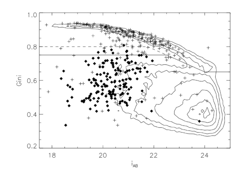
Figure 9.— The behavior of the Gini coefficient with magnitude, as shown in Figure 2, but with contours replacing the scatterplot. The stellar locus and the region occupied by galaxies are well separated. This plot has the addition of the AGN training set (crosses) and spectroscopically confirmed Narrow Emission Line Galaxies found using SDSS quasar color selection methods (diamonds). The morphological criteria adopted for this survey (shown by solid and dotted lines) exclude most NELGs while including most of the training AGN.

The set of 168 NELGs from Prescott et al. (2006) support the previously described morphological selection boundaries. The majority of the 168 NELGs (96$\%$) are well-resolved with $G<0.75$. Only 7 are accepted as AGN candidates by the low redshift Gini criteria (4$\%$) and only 1 is accepted by the high-z criteria, with $G>0.8$ ($<1\%$). Figure 9 indicates that the majority of AGN color contaminants will be cleanly separated from AGN via morphological selection. This plot shows the same data as Figure 2 (simplified to contours) but also overplots the training AGN (crosses) as well as the NLEG contaminants (diamonds). We cannot use this result in a quantitative way because the statistics might be intrinsically different at fainter magnitudes, where NELGs may be less well-resolved and so more often confused with AGN.

5. AGN SELECTION

The primary goal of targeting the AGN population is to understand the nature of low luminosity AGN evolution and spatial distribution. The AGN selection strategy can be judged in terms of targeting efficiency and completeness in recovering the predicted population. Assessing the efficiency and completeness of our algorithm depends on prior knowledge of the QLF, while also requiring additional information on the surface density of contaminating stars and galaxies down to the limiting magnitude of the AGN candidates. AGN number counts have already been discussed in §6, and a good estimate of the stellar population is given in §2.7, but the galaxy contamination is the most important and unfortunately the most difficult to assess. Defining the AGN selection algorithms is deeply dependent on the ability to estimate the efficiency of selection techniques. We used an iterative process where our selection strategy determines efficiency estimates (in this section, based solely on the training set) and efforts to improve efficiency would alter selection methods. In the following two subsections we describe how we define our selection procedure with the motivations guiding our decisions.

5.1. Low-z AGN Selection

The AGN population at $z<3$ has been well studied to $i_{AB}<22.5$, but we can target AGN candidates down to $i_{AB}=24.5$, using $G$ and $u-B$. As previously discussed, coupling these two parameters gives a clear advantage by separating galaxy, AGN, and stellar populations. In Figure 10, galaxies largely have $G<0.75$ (with starbursts at the bluer end of the distribution), stars are compact ($G>0.8$) and are relatively red with $(u-B)>\sim 0.7$ and the training set AGN, represented by diamonds on Figure 10, are generally compact (high $G$) and blue ($u-B<0.7$). Table 3 shows a flow chart of the low-z selection algorithm, which is described below.

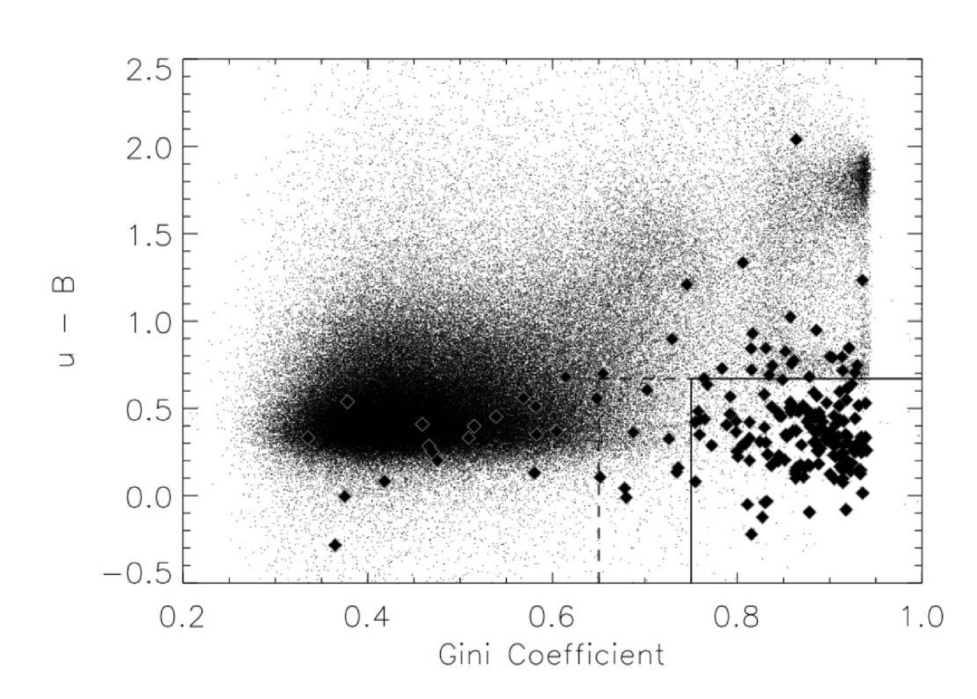
Figure 10.— Color and morphological properties can distinguish the majority of AGN from their stellar and galaxy contaminants. In this case, the separation is presented in terms of $G$ vs. $u-B$. The galaxies (thet cloud of small dots to the left) have $G<0.75$, the stars (the smaller collection of dots at the top right) has high $G$ but primarily $u-B>0.67$, and the AGN (diamonds) are more compact than almost all galaxies and bluer than almost all stars. There is a small set of well resolved AGN galaxies for which this selection is not effective due to heavy overlap with the blue end of the galaxy locus, primarily starburst galaxies, as well as a number of AGN with colors similar to the hottest stars.

Table 3Low Redshift AGN Candidate Selection Process.

$N_{Obj}$	Process	Details
195706	Objects in the CMC
190316	u, b are detections
188553	Brightness criterion	$i_{AUTO}<25.5$
17697	Gini criterion	$0.65<G<1.0$ AND
		[$G>0.75$ OR $G>-0.067\times i_{AUTO}+2.25$]
2370	$u-B$ criterion	$-2.00<u-B<0.67$
2201	X-Ray/Training Data	Exclude XRPS and Training Sample

In this subsection (restricted to §5.1), we define the survey’s completeness and efficiency in terms of the AGN training set. Completeness is the fraction or percentage of training set AGN recovered by the selection criterion, and efficiency is the number of AGN recovered or selected relative to the number of star and galaxy contaminants. Depending on our efficiency and completeness goals we can vary the cuts in $G$ and $(u-B)$ to isolate AGN candidates. The core region we use for the candidate AGN pool is bounded by $0.75<G<1.0$ and $-0.5<u-B<0.6$. It contains 51$\%$ of the training data which is therefore an approximation to the selection completeness for $z<3$. We choose 0.75 as a lower limit on Gini (rather than the more stringent choice of 0.8) because there is a moderately-sized population of 20 AGN with $0.75<G<0.80$, and Figure 8 shows that the dispersion of $G$ at low redshift is high enough to warrant a lower boundary. The objects with marginally high $G$ could be at the Seyfert/QSO boundary with visible hosts. Figure 2 highlighted the Gini selection criteria for candidates: the acceptance region for low redshift objects is above the solid line.

Another strategy would be to accept candidates with $u-B<0.1$ and all values of $G$, to recover some of the bluest and most well-resolved, low-z AGN from the training set. Although this added region does recover 7 training set AGN, there is a sharp increase in number of contaminants (resulting in a 150$\%$ increase in number of candidates) as the selection skirts the blue edge of the large galaxy population (primarily starbursts). Since the anticipated gain in completeness is small, only 2$\%$, we do not include this region in AGN candidate selection.

The final aspect of the low-z selection is to set an upper bound on $u-B$. While AGN and stars appear to separate most cleanly for $u-B<0.6$, many AGN have $0.6<u-B<0.9$, a region that overlaps hot main sequence stars and white dwarfs. While including this area would increase training set completeness from 51$\%$ to 61$\%$, the sharp increase in overlap with stars would dramatically reduce the efficiency. The choice of $(u-B)_{max}=0.67$ was made by defining and contrasting the training set completeness and efficiency. We measure completeness for a given $(u-B)_{max}$ as the fraction of training AGN within the bounds of our selection criteria out of the total 292 training AGN included in the sample. With the selection criteria in terms of Gini and magnitude as in Figure 2, and $u-B<(u-B)_{max}$, the completeness increases as we increase $(u-B)_{max}$. The efficiency (also a function of $(u-B)_{max}$) is measured as the number of training AGN selected over the total number of candidates accepted by the algorithm. The total number of candidates accepted includes the training set. These limited definitions of completeness and efficiency are distinct from the expected efficiency or completeness of the overall survey, which will be discussed in §6.

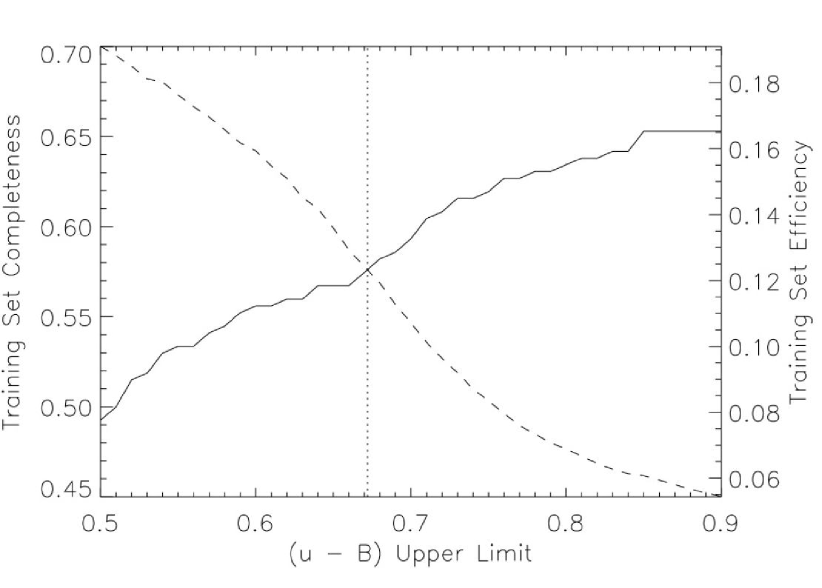
Figure 11.— Low redshift ($z<2.5$) AGN selection completeness from the training set (solid line) increases as a function of the upper bound, $(u-B)_{max}$. The efficiency from the training set (dashed line) decreases over the same range of upper bounds since the region has a high density of hot stars. The intersection of these two quantities occurs at $(u-B)_{max}=0.67$ (dotted vertical line), which is chosen as the upper bound on the low-z acceptance region.

The region in question ($0.6<u-B<0.9$) contains a sizable fraction of the $2.3<z<3.0$ AGN which are historically difficult to target. Figure 11 shows a plot of the training set completeness and fractional training set efficiency as functions of $(u-B)_{max}$. The training set completeness increases with $(u-B)_{max}$ while the efficiency decreases. Their intersection at $(u-B)_{max}=0.67$ defines the best upper bound on low-z color selection.

Noting the evolution of AGN color as a function of redshift (Figure 6), we see that beyond $z\simeq 2.5$, $u-B$ for most AGN reddens very quickly (entering the stellar locus), and this selection is no longer effective. This foreshadows why the high-z selection algorithm must use more than one color. The solid line outlines our selection criteria for the brightest candidate objects ($i_{AB}>22.5$), and the dashed line extends the region to lower $G$ for fainter candidates only (the Gini-magnitude selection for low redshift objects is illustrated in Figure 2 by the solid line). The low-z selection algorithm recovers 169 of the original 292 training AGN (58$\%$), and yields a total of 2201 candidates across the 2 deg² COSMOS field.

5.2. Intermediate-z and High-z AGN Selection

Unlike the low-z selection method, no single color can effectively be used to target $z>2.5$ AGN; strong contamination by the stellar locus makes that impossible. At $z>3$, there are no training data of spectroscopically confirmed AGN, so we rely exclusively on the AGN template predictions illustrated in Figure 6 and number counts from the X-Ray point sources with high $G$ (there are 444 above the high-z line in Figure 2). Since the X-Ray sources are not guaranteed to be AGN (knowing only $\sim$50$\%$ are type 1), their use in designing the selection algorithm is loose, and only implimented as a guide supplimenting the use of templates. We group the intermediate redshift ($2.5<z<3.0$, dubbed int-z) selection together with the high redshift selection ($z>3$) since they use the same variables and act as two subsections of a larger selection technique. Below we describe this overall technique, and split into the two redshift regimes when it is clear that the separation is needed.

Figure 12.— Selecting from the same catalog as for Figure 10, the use of a redder baseline and a similar selection technique for high-z AGN as for low-z AGN is inefficient; the overlap of predicted AGN colors (straight lines marked with redshift) with the stellar locus is severe. The 90$\%$ confidence interval on AGN template colors is shown in the upper left. This single color technique (e.g. defining the acceptance region by $V-i<0.1$ and $G>0.8$) rejects $z>3.0$ AGN 60$\%$ of the time and admits large numbers of contaminating stars.

To select objects with $z>2.5$ we need more color information than was used to define our low redshift algorithm. Figure 12 shows the expected $V-i$ color of high-z AGN, along with the same galaxy and star populations as shown in Figure 10. Overlap with the stellar locus is severe in the redshift range we are targeting, and does not let up until $z\sim 5$. Although we could avoid this problem by using an even redder baseline (e.g. $V-z$, $r-z$, or $z-K$), the limited depth of the catalogs and the photometric errors in these bands make faint, high redshift AGN selection impossible. Instead, we incorporate a second optical color, $B-V$, which goes much deeper than the redder bands (refer to Table 1 for limiting magnitudes) and which, when coupled with $V-i$, shows promising separation between the stellar locus and AGN template color predictions for $z>2.5$. To step through the stages in the int-z and high-z selection the reader should refer to Table 4.

Table 4Intermediate and High Redshift AGN Candidate Selection Process

$N_{Obj}$	Process	Details
195706	Objects in the CMC
192230	Brightness Criterion	$i_{AUTO}<25.5$
18475	$Gini$ Criterion	$0.65<G<1.00$ AND
		[$G>0.80$ OR $G>-0.067\times i_{AUTO}+2.25$]
594	High-z Selection in $(B-V)(V-i)$	$(V-i)\leq 1.15\times(B-V)-0.31$
515	High-z: Remove Training Data	Exclude XRPS and Training Sample
702	High-z: Add Blue Dropouts	Include 187 Blue Dropout Objects
1188	Int-z Selection in $(B-V)(V-i)$	$V-i>1.15\times(B-V)-0.31$ AND [$V-i<0.15$ OR
		[$V-i<0.5$ AND $V-i>1.4\times(B-V)+0.1$]]
913	Int-z: Remove Training Data	Exclude XRPS and Training Sample

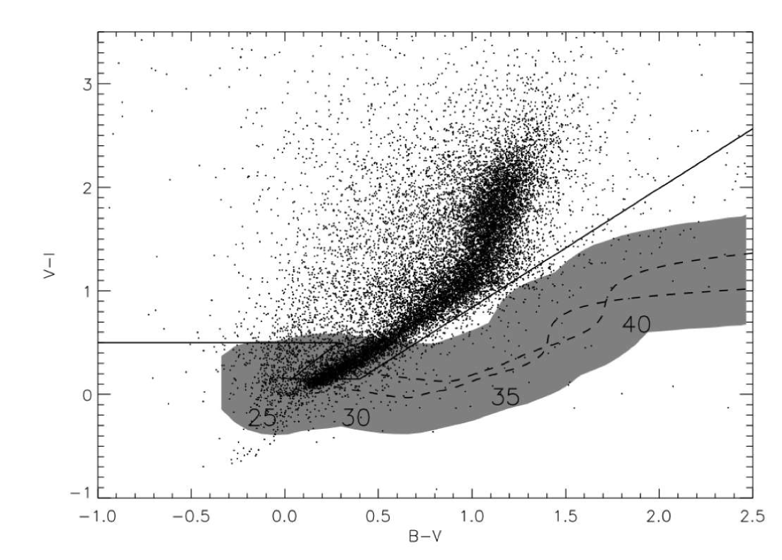
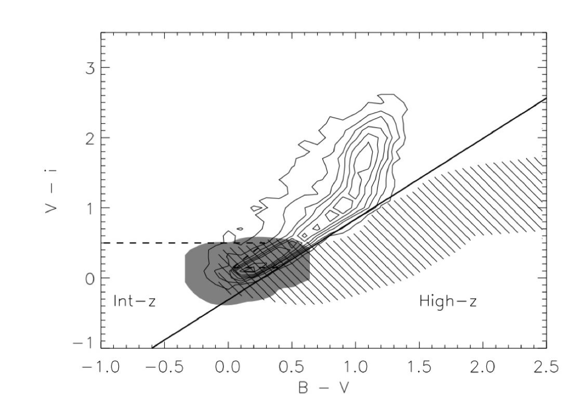
Figure 13.— $B-V$ and $V-i$ are used to select AGN with $z>2.5$, with the addition of a prior cut on Gini shown in Figure 2 by the dashed line. Without any training data above $z=3.0$, templates are used to extrapolate the colors of AGN at high redshift. The two best-fitting type 1 AGN templates (relative to low z AGN in the same colors) are shown in the top panel (dashed lines) and marked at redshifts 2.5, 3.0, 3.5 and 4.0 by “25”, “30”, “35”, and “40.” The striped region is the 90$\%$ envelope for potential AGN colors, adopted from the variance in $B-V$ and $V-i$ of the training set AGN (for lack of better information at high redshift, variance is assumed to be constant). The bottom panel shows contours converted from the scatter plot in the upper panel, and the template regions divided into intermediate redshift (gray shaded) and high redshift (striped) regions. The solid line is the upper bound on the acceptance region of the high redshift selection, while the dashed line represents the upper bound of the intermediate redshift selection (bound on bottom by the solid line). X-Ray Point sources are used roughly to guide selection, but on these plots their distribution would resemble a scatter plot adding little visual information.

The goal of the selection algorithm is to define the optimal AGN color domain without accepting significant numbers of stellar contaminants. At high redshift, AGN are generally redder, fainter, and more likely to be unresolved. This final assumption is based on both our small training set behavior, and the physical and observational constraints at high redshift. Therefore (coupled with data shown in Figure 8), we require $G>0.8$ for intermediate and high redshift candidates. The full high-z $G$ acceptance area is shown in Figure 2 as the region above both the solid and dashed lines; these objects make up the initial int-z and high-z candidate sample, and they are shown in the upper panel of the ($B-V$)($V-i$) diagrams in Figure 13. The gray area represents a 90$\%$ envelope of all AGN template predictions for $z>2.5$ (the redshifts are marked by “25”, etc.). The central lines indicate the two best fit AGN template paths through the color plane (best fit lines to $B-V$ and $V-i$ as shown in Figure 6). The bottom panel of Figure 13 shows the int-z and high-z selection methods in relation to template predictions and the stellar locus, and are described sequencially below. The area shaded by horizontal lines in the bottom panel of Figure 13 represents the $z>3.0$ AGN population outlined by templates (our high-z selection), while the area shaded by diagonal lines (spaced widely) represents the $2.5<z<3.0$ AGN population (our int-z selection). The stellar locus is converted into a contour plot to schematically show areas of high stellar contamination. Compact X-Ray point sources, while not guaranteed to be AGN, are overplotted as diamonds to supplement the areas highlighted by templates.

For efficient selection at $z>3$ we make a diagonal cut in the two color diagram, described by the line $V-i<1.15\times(B-V)-0.31$ (shown in the plot as a heavy solid line). The region below this line contains 594 objects and 54 X-Ray sources (12$\%$ of all 444 X-Ray sources considered for high-z selection), and a significant portion of the 90$\%$ AGN color envelope for $z>3$, justifying the criterion for the high-z candidate pool. There are 594 high redshift objects in this selection area, 13$\%$ of which are X-Ray sources. After removing all X-Ray sources and training data from the selected objects, there are 515 candidates for the high-z selection algorithm.

The intermediate redshift AGN occupy the area at the base of the stellar locus, blueward of the heavy diagonal line defining the high-z selection area. Contamination in this region is increased greatly by the population of hot main sequence stars and white dwarfs on the blue end of the stellar locus. Since contamination is expected to be much higher at these redshifts, we treat intermediate redshift AGN candidates separate from the high redshift AGN candidates we discussed in the previous paragraph. The region bounded by $(V-i)<0.15$ and $V-i>1.15\times(B-V)-0.31$ (the heavy line) consists of 814 objects, 93 of which are X-Ray sources (21$\%$ of the X-Ray sample). The upper limit $(V-i)_{max}=0.15$ was chosen in a similar way to $(u-B)_{max}$ from §5.1, since the anticipated contamination rate greatly increases for redder values of $V-i$. We include another region in the intermediate redshift selection by realizing that many X-Ray sources are bluer than the galaxy/star locus and that templates predict that intermediate redshift AGN will occupy the $V-i<0.5$ and $V-i>1.4\times(B-V)+0.1$ area. This adds 374 more candidates and 115 more X-Ray sources (up to 46$\%$ of the X-Ray sample). The total number of intermediate redshift AGN candidates is 913 after removing X-Ray sources and the training set (from an original 1188). The acceptance region for int-z selection is shown on the bottom panel of Figure 13 enclosed by the heavy dashed line and solid line.

One final catagory of targets is considered as potential high redshift AGN. We have included 187 blue dropouts, where $i$ band is a detection, but $B$ band is not. These are interesting because of their very red color ($B-i>2$) and faint magnitude ($i_{AB}\sim 24.0$), which potentially corresponds to very high redshift AGN, in the range $3.4<z<5.5$. There are only 638 blue dropouts in the entire COSMOS catalog, of which 187 satisfy the high-z Gini cut described in §4. We add these objects into the high-z candidate list, bringing the total number up to 702.

6. Estimating Population Statistics and Algorithm Efficiency

Because we have not yet carried through with spectroscopic observations of our candidates, we cannot directly or reliably predict our algorithms’ efficiency or completeness. Instead we carefully construct a contextual arguement by roughly estimating quasar, star, and galaxy population statistics. By comparing our selection technique to other current algorithms in the literature, we estimate efficiency at $\sim$30-50$\%$ and completeness $>$60$\%$. While detailed runs of Monte Carlo simulations could be used to estimate this completeness more precisely, that is not the focus of this paper. Instead a follow-up paper detailing the yeilds of this study will more carefully explore our method’s robustness in choosing low-luminosity AGN or potentially faint high redshift AGN in the future.

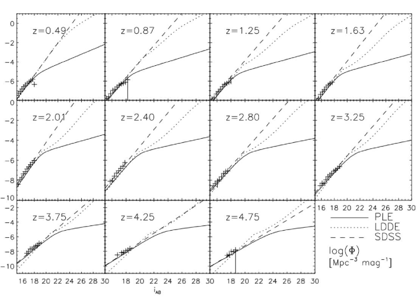
Figure 14.— The Quasar Luminosity Function behavior at selected redshifts for the PLE model (solid), LDDE model (dotted), and the bright end QLF derived by Richards et al. (2006) (dashed) from the SDSS DR3 quasar counts (crosses). These were calibrated through bolometric corrections to agree at the bright end (the realm of SDSS data) with divergence at the faint end. The QLF models produce diverse predictions of the number counts of quasars at the faint level of COSMOS.

The Quasar Luminosity Function (QLF) has been studied extensively over the past decade with an increasing range of statistics used to verify some descriptive functional forms, like the double power law (e.g. Pei, 1995; Peterson, 1997; Boyle et al., 2000; Croom et al., 2004), which may be used to generate a prediction of the faint end QLF out to $z\sim 6$. The most useful treatments and observational insights into the QLF in the literature turn out to be inappropriate for the range of magnitudes we need (Richards et al., 2005, 2006; Jiang et al., 2006). We use the pure luminosity evolution (PLE) model of Hopkins, Richards, & Hernquist (2007), who tied together several data sets for the best faint end reliability, where most of our tarets lie. The luminosity-dependent density evolution (LDDE) model is also often used to describe the QLF, however, at the faintest magnitudes we suspect it overestimates the quasar counts by $\sim$2dex and is inappropriate in this context. The predicted QLFs (PLE and LDDE) are shown in Figure 14. The predicted AGN number counts for the COSMOS field (from these QLFs at various redshifts) are shown in Figure 15, with 1$\sigma$ errors propagated from the error in the QLFs.

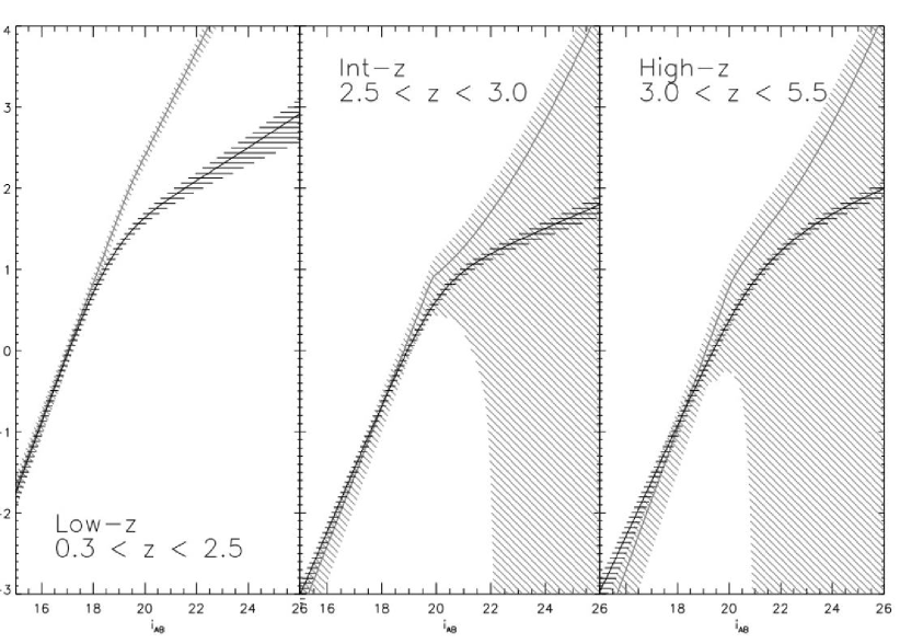
Figure 15.— The predicted number counts of quasars in the COSMOS field (1.7 square degrees) for the low redshift interval ($0.3<z<2.4$), the intermediate redshift interval ($2.5<z<3.0$), and the high redshift interval ($3.0<z<5.5$). The PLE quasar number counts are given by the black line, with the 1$\sigma$ margin of error as the horizontally shaded regions. The LDDE model is represented by the gray line with the 1$\sigma$ diagonal shaded region; at high redshifts and at faint magnitudes, the LDDE quasar number count is not well constrained and does not have a lower limit. This reinforces the need to target faint AGN$-$so the QLF may be more well constrained in regimes where little data exists today.

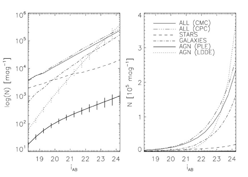
Figure 16.— Logarithmic and linear plots of the expected number counts of objects in the candidate pool. The solid line represents all objects in the CMC, while the triple-dot-dashed line shows the parent distribution of objects in the CPC of the same magnitude range (see Figure 1). The stellar population identified by Robin et al. (2007) is shown as the dashed line and at the faintest magnitudes, constituting about 10$\%$ of the CMC contents. An estimate of galaxy counts is shown as the dot-dashed line and is given in Capak et al. (2007) referencing previous galaxy count work from COSMOS, H-HDF-N, HDF-N, HDF-S, Herschel, SDSS, CFDF, and CFHT (Leauthaud et al., 2007; Capak et al., 2004; Williams et al., 1996; Metcalfe et al., 2001; Yasuda et al., 2001; McCracken et al., 2003, 2007). The predicted QLF counts (from Figure 15) are shown with appropriate error bars$-$PLE as the heavy solid line and LDDE as the dotted line. The LDDE formulation is inappropriate at the faintest magnitudes where it predicts that quasars would constitute the entire contents of the catalog. Therefore the PLE formulation of the QLF (of order 1$\%$ of the CMC number counts) is adopted.

Figure 16 gathers all predictive number counts for QSOs, stars (Robin et al., 2007), and galaxies (Capak et al., 2007) in relation to the number counts of objects in the CMC catalog. At the faint level of this survey, it is well known that AGN and stars are minor components of a population that is made up primarily of galaxies. The galaxy count (not previously discussed) given in the latter reference is based on external measures of the galaxy surface density, which agrees with several other surveys up to 80$\%$ completeness at $i=26.5$ This shows the overwhelming statistics of the galaxy population with respect to stars and AGN. Figure 17 shows the stellar contaminants relative to the total number of selected objects as well as predicted QLF AGN densities from the PLE method. Galaxy predictions are not shown because of their huge numbers, thus they cannot be reliably determined. Relative to the AGN counts, the stellar contaminants are roughly 3-4 times more numerous at low redshift and $\sim$10 times more numerous at high redshift and hypothetically constitute $\sim$1/2 of all selected candidates (although given our methodology biases against stellar selection, this is highly unlikely).

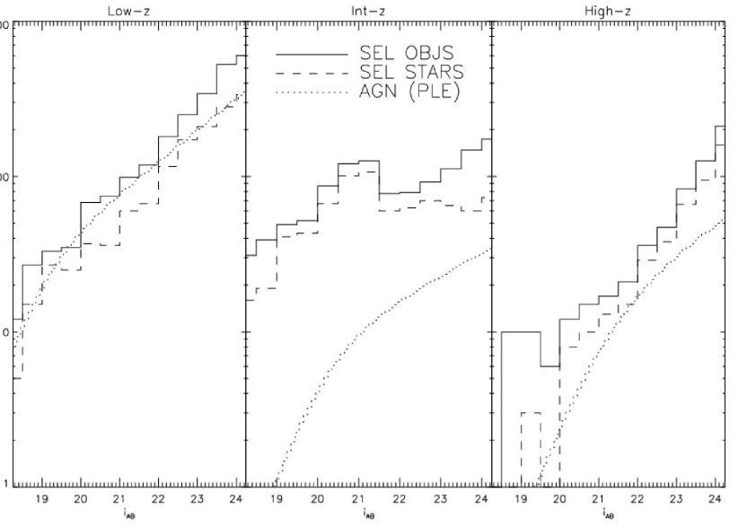
Figure 17.— The magnitude distribution of all selected objects (solid line) through the different redshift algorithms. The selected stars are shown as a dashed line, which constitute about 5$\%$ of the overall stellar population from Robin et al. (2007), and $\sim$50$\%$ of all selected objects. The QLF count predictions (dotted line) show the AGN numbers relative to the total number of selected objects. The contamination from faint blue, compact galaxies can be inferred from this information (subtracting stars from the total) but there is no reliable method to measure those numbers.

A recent study by Siana et al. (2007) presents an optical and IR selection technique of QSOs at high-z down to $i\sim 22$. When coupled with results from confirming spectroscopy of $\sim$10 QSOs, they conlude a completeness of 80 - 90$\%$ using detailed Monte Carlo simulations. This estimate is based on the premise that QSOs likely exhibit colors of QSO templates and are selected by their paths in color-color space, which differ from stellar contaminants. Using this methodology, we make a very similar conclusion based on the similarities of our techniques: at high redshift ($z>3$), our selection algorithm as shown in Figure 13 will have a high completeness ($>$60$\%$). A thorough assessment of this success rate will be included in a follow-up paper detailing observational results and yields.

To test the bounds on completeness and efficiency, we run the selection on the XRPS sample population (which is likely comprised of 90$\%$ AGN, but only $\sim$50$\%$ type 1 AGN) and compute efficiency and completeness for this sample. The 1073 X-Ray point sources introduced in §2.5, were not useful in designing the algorithms, but they may now be used retrospectively to probe the efficiency and completeness. We add the selected X-Ray point sources back into the selected objects (modification of the last steps in Tables 3 and 4), and then compute the efficiency and completeness with respect to these X-Ray objects. Altogether, 323 X-Ray sources are targeted by the low-z algorithm and 203 are targeted in int-z, and 57 using the high-z technique. The relative completeness and efficiency of the algorithms targeting the X-Ray point sources may be seen in Figure 18. Low yeilds at faint magnitudes are potentially misleading since far fewer XRPS are at such faint magnitudes. The completeness rate here must also not be misinterpreted$-$it represents the fraction of the 1073 XRPS which are selected by the low-z, int-z, and high-z algorithms. Since the XRPS likely consist of very few high redshift objects (Trump et al., 2007), the low completeness calculation for high-z is expected (upper right panel of Figure 18), but as shown, the algorithm is very efficient in selecting those XRPS which are suspected to be high-z sources (lower right panel of Figure 18). The algorithms are fairly successful in selecting and targeting such faint optical objects with efficiencies as high as 50$\%$ and completeness as high as 40$\%$. The X-Ray point sources are already known to be probable AGN, but this test shows that the selection methodology is able to successfully target AGN with reasonable yield statistics.

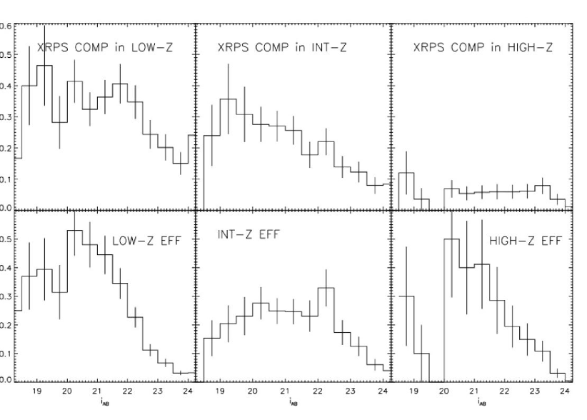
Figure 18.— The completeness (top panels) and efficiencies (bottom panels) of the algorithms as defined by the X-Ray point sources. Note that the completeness represented in each upper panel is the number of selected objects in each algorithm divided by 1073, the total number of XRPS, and does not relate to predictions from the QLF. While only 57 XRPS are selected in high-z (low completeness for XRPS), the efficiency is quite high. While it only is representative of a subset population which likely consists of low-z sources, it is valuable in understanding the true effectiveness of each technique.

7. Conclusions

The method described by this paper aims to probe the faint end of the quasar luminosity function via optical AGN selection; it is framed by complex effects of a dominant contaminating population of faint stars and galaxies. Pushing optical selection to this faint level ($i\sim 24.5$) requires extensive knowledge of stellar colors, stellar number counts, galaxy color contamination, compact galaxies, AGN color and morphology properties, and reliable predictions of counts from the evolving quasar luminosity function. This paper establishes optical AGN selection methods for the COSMOS field (with photometry from ground-based Subaru and CFHT, along with Hubble ACS imaging) using data on spectroscopically confirmed AGN, X-Ray point sources, AGN color templates, and stellar studies done in the COSMOS field. We have discussed and accounted for the color of both AGN and contaminating stellar and starburst galaxy populations, the use of the Gini coefficient as a reliable discriminant between point sources likely to be AGN or stars and extended galaxies, and the evolution of both color and morphology as functions of redshift and magnitude. While the color of blue galaxies at all magnitude levels dominates the AGN contamination, leverage from the Gini coefficient can significantly hinder the effect of this contamination on unresolved AGN galaxies (while being defenseless to select against compact blue galaxies).

The method of targeting AGN was split into three sections: one for low redshift AGN ($z<2.5$), one for intermediate redshift AGN ($2.5<z<3.0$), and another for high redshift AGN ($z>3.0$). The low and high redshift selections straddle the redshift regime of $2.5<z<3.0$ where AGN colors resemble those of A stars in every band, and are therefore indistinguishable from stellar contaminants. We design a method to target these intermediate redshift AGN, but the selection is significantly hindered by increased contamination rates when compared to the low-z and high-z algorithms. The low redshift algorithm was based on the bluest baseline, $u-B$, and the Gini coefficient. The low-z AGN were identified as consistently bluer than most stars and more compact than most galaxies. The high redshift algorithm used more than one color to identify AGN, adopting $B-V$ and $V-i$. It relied on predictions from AGN templates to predict the color properties of AGN, but also used the Gini coefficient to eliminate extended sources from the candidate pool. We design the intermediate redshift selection as a branch of the high redshift selection; it is important to target these redshifts since it is known that AGN are more numerous in the range $2.5<z<3.0$ than at higher redshift. It is more advantageous to design a separate int-z algorithm to accept heavier contamination from stars than miss this AGN population completely.

The selection algorithms are designed to maximize both completeness and efficiency of selecting faint AGN. Although these quantities can only be estimated in advance of confirming spectroscopy of selected candidates, the experiment has proven successful in its ability to recover a test sample of X-Ray point sources (which are known to be $\sim$90$\%$ AGN, and $\sim$50$\%$ type 1 AGN). With $\sim$2700 low redshift candidate objects, $\sim$1000 intermediate redshift objects and $\sim$600 high redshift candidates in the 2 deg² COSMOS field, the method could hypothetically recover $\sim$700 low-z AGN, $\sim$200 int-z AGN, and $\sim$200 high-z AGN. As a conservative estimate, roughly 2 to 10 candidates will have to be observed to identify each new AGN. A total of $\sim 160$ candidates have been observed at Magellan IMACS and LDSS3 as of May 2007 and more observations are planned.

References

- Abraham et al. (2003) Abraham, R. G., van den Bergh, S., & Nair, P. 2003, ApJ, 588, 218
- Abraham et al. (2004) Abraham, R. G., et al. 2004, AJ, 127, 2455
- Abraham et al. (2007) Abraham, R. G., et al. 2007, ApJ, 669, 184
- Bahcall & Soneira (1981) Bahcall, J. N., & Soneira, R. M. 1981, ApJS, 47, 357
- Beckwith et al. (2006) Beckwith, S. V. W., et al. 2006, AJ, 132, 1729
- Benítez (1999) Benítez, N. 1999, in Astronomical Society of the Pacific Conference Series, Vol. 191, Photometric Redshifts and the Detection of High Redshift Galaxies, ed. R. Weymann, L. Storrie-Lombardi, M. Sawicki, & R. Brunner, 31
- Bertin & Arnouts (1996) Bertin, E., & Arnouts, S. 1996, A&AS, 117, 393
- Bigelow et al. (1998) Bigelow, B. C., Dressler, A. M., Shectman, S. A., & Epps, H. W. 1998, in Presented at the Society of Photo-Optical Instrumentation Engineers (SPIE) Conference, Vol. 3355, Proc. SPIE Vol. 3355, p. 225-231, Optical Astronomical Instrumentation, Sandro D’Odorico; Ed., ed. S. D’Odorico, 225–231
- Boyle et al. (2000) Boyle, B. J., Shanks, T., Croom, S. M., Smith, R. J., Miller, L., Loaring, N., & Heymans, C. 2000, MNRAS, 317, 1014
- Brusa et al. (2006) Brusa, M., et al. 2006, ArXiv Astrophysics e-prints
- Brusa et al. (2007) —. 2007, ApJS, 172, 353
- Budavári et al. (2001) Budavári, T., et al. 2001, AJ, 122, 1163
- Capak et al. (2004) Capak, P., et al. 2004, AJ, 127, 180
- Capak et al. (2007) Capak, P., et al. 2007, ApJS, 172, 99
- Cappelluti et al. (2007) Cappelluti, N., et al. 2007, ApJS, 172, 341
- Chen et al. (1999) Chen, B., Figueras, F., Torra, J., Jordi, C., Luri, X., & Galadí-Enríquez, D. 1999, A&A, 352, 459
- Chen et al. (2001) Chen, B., et al. 2001, ApJ, 553, 184
- Croom et al. (2001) Croom, S. M., Smith, R. J., Boyle, B. J., Shanks, T., Loaring, N. S., Miller, L., & Lewis, I. J. 2001, MNRAS, 322, L29
- Croom et al. (2004) Croom, S. M., Smith, R. J., Boyle, B. J., Shanks, T., Miller, L., Outram, P. J., & Loaring, N. S. 2004, MNRAS, 349, 1397
- Fan (1999) Fan, X. 1999, AJ, 117, 2528
- Foltz et al. (1987) Foltz, C. B., Chaffee, Jr., F. H., Hewett, P. C., MacAlpine, G. M., Turnshek, D. A., Weymann, R. J., & Anderson, S. F. 1987, AJ, 94, 1423
- Gini (1912) Gini, C. 1912, reprinted in Memorie di Metodologia Statistica, ed. E. Pizetti T. Salvemini (1955; Rome: Libreria Eredi Virgilio Veschi)
- Hall et al. (1996) Hall, P. B., Osmer, P. S., Green, R. F., Porter, A. C., & Warren, S. J. 1996, ApJ, 462, 614
- Hasinger et al. (2006) Hasinger, G., et al. 2006, ArXiv Astrophysics e-prints
- Hasinger et al. (2007) —. 2007, ApJS, 172, 29
- Hewett et al. (1995) Hewett, P. C., Foltz, C. B., & Chaffee, F. H. 1995, AJ, 109, 1498
- Hogg (1999) Hogg, D. W. 1999, ArXiv Astrophysics e-prints
- Hopkins et al. (2007) Hopkins, P. F., Richards, G. T., & Hernquist, L. 2007, ApJ, 654, 731
- Jiang et al. (2006) Jiang, L., Fan, X., Cool, R. J., Eisenstein, D. J., Zehavi, I., Richards, G. T., Scranton, R., Johnston, D., Strauss, M. A., Schneider, D. P., & Brinkmann, J. 2006, AJ, 131, 2788
- Koo & Kron (1982) Koo, D. C., & Kron, R. G. 1982, A&A, 105, 107
- Leauthaud et al. (2007) Leauthaud, A., et al. 2007, ApJS, 172, 219 Leauthaud, A., et al. 2007, submitted to ApJS
- McCracken et al. (2003) McCracken, H. J., Radovich, M., Bertin, E., Mellier, Y., Dantel-Fort, M., Le Fèvre, O., Cuillandre, J. C., Gwyn, S., Foucaud, S., & Zamorani, G. 2003, A&A, 410, 17
- McCracken et al. (2007) McCracken, H. J., et al. 2007, ArXiv e-prints, 704
- Metcalfe et al. (2001) Metcalfe, N., Shanks, T., Campos, A., McCracken, H. J., & Fong, R. 2001, MNRAS, 323, 795
- Mobasher et al. (2006) Mobasher, B., et al. 2006, ArXiv Astrophysics e-prints
- Pei (1995) Pei, Y. C. 1995, ApJ, 438, 623
- Peterson (1997) Peterson, B. M. 1997, An Introduction to Active Galactic Nuclei (An introduction to active galactic nuclei, Publisher: Cambridge, New York Cambridge University Press, 1997 Physical description xvi, 238 p. ISBN 0521473489)
- Prescott et al. (2006) Prescott, M. K. M., Impey, C. D., Cool, R. J., & Scoville, N. Z. 2006, ApJ, 644, 100
- Reid & Majewski (1993) Reid, N., & Majewski, S. R. 1993, ApJ, 409, 635
- Richards et al. (2001) Richards, G. T., et al. 2001, AJ, 121, 2308
- Richards et al. (2002) —. 2002, AJ, 123, 2945
- Richards et al. (2004) —. 2004, ApJS, 155, 257
- Richards et al. (2005) —. 2005, MNRAS, 360, 839
- Richards et al. (2006) —. 2006, AJ, 131, 2766
- Robin et al. (2007) Robin, A. C., et al. 2007, ApJS, 172, 545
- Sandage & Wyndham (1965) Sandage, A., & Wyndham, J. D. 1965, ApJ, 141, 328
- Schinnerer et al. (2007) Schinnerer, E., et al. 2007, ApJS, 172, 46
- Schmidt & Green (1983) Schmidt, M., & Green, R. F. 1983, ApJ, 269, 352
- Schneider et al. (2007) Schneider, D. P., et al. 2007, AJ, 134, 102
- Scoville et al. (2007) Scoville, N., et al. 2007, ApJS, 172, 1
- Siana et al. (2007) Siana, B., et al. 2007, ArXiv e-prints, 711
- Spergel et al. (2003) Spergel, D. N., et al. 2003, ApJS, 148, 175
- Trump et al. (2007) Trump, J. R., et al. 2007, ApJS, 172, 383
- Warren et al. (1991) Warren, S. J., Hewett, P. C., & Osmer, P. S. 1991, ApJS, 76, 23
- Williams et al. (1996) Williams, R. E., et al. 1996, AJ, 112, 1335
- Yasuda et al. (2001) Yasuda, N., et al. 2001, AJ, 122, 1104
- York et al. (2000) York, D. G., et al. 2000, AJ, 120, 1579