The Effect of Charon’s Tidal Damping on the Orbits of Pluto’s Three Moons

Abstract

Pluto’s recently discovered minor moons, Nix and Hydra, have almost circular orbits, and are nearly coplanar with Charon, Pluto’s major moon. This is surprising because tidal interactions with Pluto are too weak to damp their eccentricities. We consider an alternative possibility: that Nix and Hydra circularize their orbits by exciting Charon’s eccentricity via secular interactions, and Charon in turn damps its own eccentricity by tidal interaction with Pluto. The timescale for this process can be less than the age of the Solar System, for plausible tidal parameters and moon masses. However, as we show numerically and analytically, the effects of the 2:1 and 3:1 resonant forcing terms between Nix and Charon complicate this picture. In the presence of Charon’s tidal damping, the 2:1 term forces Nix to migrate outward and the 3:1 term changes the eccentricity damping rate, sometimes leading to eccentricity growth. We conclude that this mechanism probably does not explain Nix and Hydra’s current orbits. Instead, we suggest that they were formed in-situ with low eccentricities.

We also show that an upper limit on Nix’s migration speed sets a lower limit on Pluto-Charon’s tidal circularization timescale of $>10^{5}\,$ yrs. Moreover, Hydra’s observed proper eccentricity may be explained by the 3:2 forcing by Nix.

1. Introduction

Weaver et al. (2006) discovered two small moons orbiting Pluto. These moons—Nix and Hydra—are much less massive than Pluto’s major moon Charon, whose mass relative to Pluto’s is $M_{C}/M_{P}\simeq 0.12$ (Buie et al., 2006), whereas Nix and Hydra’s masses are $M_{N}/M_{P}=(4\pm 4)\times 10^{-5}$ and $M_{H}/M_{P}=(2\pm 4)\times 10^{-5}$, based on a 4-body fit to the observed positions (Tholen et al., 2007b). Weaver et al. (2006) also found that (a) the orbits of Nix and Hydra are nearly circular and coplanar with Charon; and (b) the period ratios of Charon:Nix:Hydra are nearly 1:4:6. By analyzing earlier data taken over a year-long interval and fitting the data to Keplerian orbits around a point mass, Buie et al. (2006) showed that (a) Nix and Charon’s eccentricities are consistent with zero, with $e_{N}=0.0023(21)$ and $e_{C}=0.00000(7)$ where brackets denote 1-$\sigma$ errors in the trailing digits, but Hydra’s formally is not, with $e_{H}=0.0052(11)$; and (b) the period ratio of Charon:Nix:Hydra is 1:3.8915(2):5.9817(2). Recently Tholen et al. (2007b) performed a full four-body fit to the moons’ positions, and thereby obtained slightly different orbital parameters. We discuss some of their results in §3.

Hopefully, Nix and Hydra’s remarkable orbital properties can teach us something about how they formed, perhaps shedding light on the formation of Kuiper belt objects in general. The near circularity and coplanarity is surprising. If Nix and Hydra formed in the collision that produced Charon, they likely had high eccentricities and inclinations just after formation. Nix and Hydra cannot damp their eccentricities through tidal interactions with Pluto—the corresponding damping times, for typical parameters, are at least $10^{3}$ times longer than the age of the Solar System (also see Stern et al., 2006).

Ward & Canup (2006) propose a scenario that not only accounts for Nix and Hydra’s low eccentricities and inclinations, but also accounts for their near-resonant orbits. In their “forced resonant migration” scenario, Nix and Hydra formed in the impact that produced Charon. Immediately after impact, all three moons were much closer to Pluto than they are today, and Nix and Hydra’s eccentricities were damped by a disk of post-impact debris. Subsequently, Charon migrated outwards by raising tides on Pluto, and it forced Nix and Hydra to migrate as well because they were trapped in its 4:1 and 6:1 corotation resonances. Just before Charon stopped migrating, it left Nix and Hydra at their current positions. Although this is a neat scenario, we show in a forthcoming paper (Lithwich & Wu, in preparation) that it cannot work. The difficulty is that Charon cannot simultaneously force both Hydra and Nix to migrate. To transport Nix, Charon’s eccentricity must satisfy $e_{C}<0.024$; otherwise, the 4:1 corotation resonance is destroyed by resonance overlap, as we prove with numerical simulations. But to transport Hydra, it is required that $e_{C}>0.1$; otherwise, the width of the 6:1 resonance is so small that the time for the resonance to sweep across Hydra is shorter than the libration time within the resonance. Because these two constraints are incompatible, the Ward & Canup (2006) scenario cannot work.

But Nix and Hydra can damp their eccentricities in a different way that has not been considered previously: they can transfer their eccentricity to Charon via secular interactions, and since Charon damps its own eccentricity relatively quickly through its own tidal interactions with Pluto, this process can damp eccentricities faster than the direct interaction of Nix or Hydra with Pluto. We shall show below that the timescale for this process for Nix is (eq. [44])

$$2.7\tau_{C}{M_{C}\over M_{N}},$$ (1)

where $\tau_{C}$ is Charon’s eccentricity damping time. The value of $\tau_{C}$ is somewhat uncertain. If one assumes that Pluto and Charon are consolidated ice spheres with material strength of $4\times 10^{10}$erg/cm³, then $\tau_{C}\sim 5(Q/100)$ Myr (Goldreich, 1963; Dobrovolskis et al., 1997), where $Q$ is either Pluto’s or Charon’s tidal damping parameter. (Both Pluto and Charon contribute comparably to $\tau_{C}$.) Taking $\tau_{C}=5$ Myr, equation (1) implies that the damping timescale is less than the age of the Solar System if $M_{N}/M_{P}\gtrsim 3\times 10^{-4}$. Given the uncertainties in $\tau_{C}$—for example, $Q$ could be $\ll 100$, or Charon might be a rubble pile instead of a consolidated ice sphere, which would increase its tidal Love number and decrease $\tau_{C}$—it is quite possible that the timescale of equation (1) is less than the age of the Solar System.

One is then tempted to conclude that Nix and Hydra could have formed with relatively large eccentricities, and that these were damped away as described above. However, we shall show below that, for Nix, the 2:1 and 3:1 resonant forcing terms with Charon severely complicate this picture.

2. Pluto, Charon and Nix

2.1. N-body Simulation

Figure 1 shows the result of an N-body simulation of Pluto, Charon, and Nix, with tidal damping acting on Pluto and Charon. The N-body integration is performed with the SWIFT package (Levison & Duncan, 1994), using the hierarchical Jacobi symplectic integrator of Beust (2003), and supplemented with an algorithm for tidal damping. Nix and Charon have masses $M_{N}=1.5\times 10^{-4}M_{P}$ and $M_{C}=0.1M_{P}$, respectively. To speed up the simulation, we set the circularization time of the Pluto-Charon binary to $\tau_{C}=100$ yrs. Although this is shorter than the true $\tau_{C}$ by many orders of magnitude, we shall show that all relevant timescales scale with $\tau_{C}$. Hence for more realistic values of $\tau_{C}$, one need only rescale the bottom time axis by the factor $\tau_{C}/100$ yrs.

The points in the top panel show Charon and Nix’s instantaneous eccentricities in Jacobi coordinates, and the lines show their proper eccentricities. To be more precise, the lines are the time-average of one component of the eccentricity vectors, averaged over 100 days, which is a crude way to remove the short-term noise from the eccentricities. We start Charon on a circular orbit at its current location (with a period of 6.4 days), and Nix on an orbit with an instantaneous eccentricity $0.05$ and with $a_{N}/a_{C}\sim 2.2$, where $a$ is the semi-major axis. At early times, Nix’s proper eccentricity decays. The top time axis is in units of the damping time of the slowly damped secular mode (eq. [44], which is equivalent to eq. [1]). The figure shows that Nix’s eccentricity initially damps on a timescale much faster than equation (1). But at later times, Nix’s eccentricity evolves in a complicated manner: it increases for a while before decaying again.

The bottom panel of Figure 1 shows the ratio of semimajor axes. Charon’s semimajor axis $a_{C}$ (not shown) remains virtually constant. Nix’s semimajor axis slowly increases throughout the simulation, and crosses through the nominal position of the 4:1 resonance (marked by the arrow).

Figure 1.— N-body simulation of Pluto, Charon, and Nix with tidal damping on Pluto and Charon. The simulation had tidal circularization time $\tau_{C}=100$yrs; for more realistic values of $\tau_{C}$, the bottom time axis should be rescaled by $\tau_{C}/100$yrs. The top time axis is in units of the damping time of the slowly damped secular mode (§2.3). In the top panel, the points depict Charon and Nix’s instantaneous eccentricities in Jacobi coordinates, and the solid lines depict their proper eccentricities. The lower panel displays the semi-major axis ratio between Nix and Charon, with the arrow indicating the nominal position of the $4:1$ resonance.

2.2. Simplified Model

In the remainder of this section, we explain the complicated behavior shown in Figure 1. In this subsection we introduce a simplified model, keeping only a small number of terms in the disturbing function, and show that a numerical integration of the simplified model qualitatively reproduces the behavior of Figure 1. In §§2.3-2.5, we isolate the individual terms within the simplified model, and explain their effects. The reader uninterested in the technical details may skip to a summary of our findings in §2.6.

We adopt Jacobi orbital elements, in which Nix’s elements are relative to the center-of-mass of the Pluto-Charon binary, and Charon’s elements are relative to Pluto:

$$\{a_{j},\lambda_{j},e_{j},{{\varpi}}_{j}\}\ ,\ \ j\in\{C,N\}\$$ (2)

where subscript $C$ is for Charon, or to be more accurate the Pluto-Charon binary, and $N$ is for Nix. Standard treatments of the planetary equations adopt heliocentric (equivalent here to Plutocentric) elements (Murray & Dermott, 1999). But the present problem is more suited to Jacobi elements. We show in the Appendix that using Jacobi elements changes the standard treatment in two ways. First, instead of the usual indirect term in the disturbing function, there is a different correction to the direct term, given by equation (A23) to first order in the ratio of Charon’s to Pluto’s mass ($M_{C}/M_{P}\sim 0.1$). And second, the appropriate masses must be used; for example, it is the reduced mass of the Pluto-Charon binary that enters into equation of motion. We ignore this second change in the body of the paper because we only seek an accuracy of $\sim M_{C}/M_{P}\sim 10\%.$

We model the gravitational forces on Nix and Charon with the truncated Hamiltonian

$$H=H_{{\rm unp},C}+H_{{\rm unp},N}+H_{{\rm sec},CN}+H_{2:1,CN}+H_{3:1,CN}\ .$$ (3)

These terms and their associated coefficients are defined in Tables 1 and 2, respectively, where $M_{j}$ are the masses, $\mu_{C}\equiv M_{C}/(M_{C}+M_{P})$,

$$z_{j}\equiv e_{j}e^{i{{\varpi}}_{j}}$$ (4)

are the complex eccentricities, and we choose units so that

$${{G}}(M_{P}+M_{C})=1\ .$$ (5)

The equations of motion are given by Hamilton’s equations

$${dz_{j}\over dt} = -{2i\over M_{j}\sqrt{a_{j}}}{\partial H\over\partial z_{j}^{*}}$$ (6)

$${da_{j}\over dt} = -{2\sqrt{a_{j}}\over M_{j}}{\partial H\over\partial\lambda_{j}}$$ (7)

$${d\lambda_{j}\over dt} = {2\sqrt{a_{j}}\over M_{j}}{\partial H\over\partial a_{j}}\ ,\ \ \ j\in\{C,N\}\$$ (8)

For $d\lambda_{j}/dt$, it suffices in this paper to consider only the contribution of the unperturbed energies $H_{{\rm unp},j}$, i.e.

$${d\lambda_{j}\over dt}=n_{j}\ ,$$ (9)

where

$$n_{j}\equiv a_{j}^{-3/2}$$ (10)

is the mean motion.

Both the 2:1 and the 3:1 resonant forcing terms in the Hamiltonian play important roles even when Nix and Charon are not particularly close to the nominal locations of those resonances.

We model the tidal damping of Charon’s eccentricity by adding the term

$${dz_{C}\over dt}\Big{|}_{\rm tide}\equiv-\gamma_{C}z_{C}$$ (11)

to the equation for $z_{C}$, where

$$\gamma_{C}\equiv 1/\tau_{C}$$ (12)

is Charon’s eccentricity damping rate in the absence of Nix.

Table 1 Terms in Charon-Nix Hamiltonian Used in This Paper

$H_{{\rm unp},C}=-{M_{C}\over 2a_{C}}$	Charon’s unperturbed energy
$H_{{\rm unp},N}=-{M_{N}\over 2a_{N}}$	Nix’s unperturbed energy
$H_{{\rm sec},CN}=-\mu_{C}{M_{N}\over a_{N}}\left(g_{1}\left(|z_{C}|^{2}+|z_{N}|^{2}\right)+{1\over 2}g_{2}\left(z_{C}z_{N}^{*}+z_{C}^{*}z_{N}\right)\right)$	secular interaction energy
$H_{2:1,CN}=-\mu_{C}{M_{N}\over 2a_{N}}\left(g_{3}z_{C}^{*}+g_{4}z_{N}^{*}\right)e^{i(2\lambda_{N}-\lambda_{C})}+c.c.$	2:1 resonant interaction energy
$H_{3:1,CN}=-\mu_{C}{M_{N}\over 2a_{N}}\left(g_{5}z_{C}^{*2}+g_{6}z_{C}^{*}z_{N}^{*}+g_{7}z_{N}^{*2}\right)e^{i(3\lambda_{N}-\lambda_{C})}+c.c.$	3:1 resonant interaction energy

Table 2 Coefficients in Charon-Nix Hamiltonian

$g_{1}=\alpha b_{3/2}^{1}/8$	$=0.0815$
$g_{2}=-\alpha b_{3/2}^{2}/4$	$=-0.0792$
$g_{3}=(-2-\alpha D/2)b_{1/2}^{2}$	$=-0.390$
$g_{4}=(3/2+\alpha D/2)b_{1/2}^{1}-2\alpha$	$=0.0811$
$g_{5}=(21/8+5\alpha D/4+\alpha^{2}D^{2}/8)b_{1/2}^{3}$	$=0.315$
$g_{6}=(-5-5\alpha D/2-\alpha^{2}D^{2}/4)b_{1/2}^{2}$	$=-1.41$
$g_{7}=(17/8+5\alpha D/4+\alpha^{2}D^{2}/8)b_{1/2}^{1}-27\alpha/8$	$=0.186$

Figure 2 shows the result from numerically integrating these equations of motion, where the $g_{i}$ coefficients in the Hamiltonian are evaluated at the 4:1 location (Table 2). The evolution in this simplified model is qualitatively similar to that seen in the N-body integration of Figure 1. The eccentricities initially decay, then rise, and finally decay again. And Nix’s semimajor axis increases with time.

Figure 2.— Numerical integration of the simplified model. The curves show the result from integrating equations (6), (7), and (9) with tidal damping (eq. [11]), and with the Hamiltonian given by eq. (3). The masses of Pluto, Charon, and Nix and the tidal damping rate of Charon are all the same as in the N-body simulation of Figure 1. The top panel shows the eccentricities after subtracting off the complex eccentricities forced by the 2:1 resonance (eqs. [60]-[61]). The evolution seen in this figure is qualitatively similar to that seen in Figure 1: the eccentricities first decay, then rise, then decay again. And Nix is pushed out by Charon.

2.3. Secular Evolution With Tidal Damping

To explain the behavior of the simplified model, we consider first the effect of only the secular term ($H=H_{{\rm sec},CN}$), together with tidal damping (eq. [11]). The equations of motion are then

$${d\over dt}\left(\begin{array}[]{c}z_{C}\\ z_{N}\end{array}\right)=i{{\eta}}\left(\begin{array}[]{cc}\delta&-\beta\delta\\ -\beta&1\end{array}\right)\left(\begin{array}[]{c}z_{{C}}\\ z_{N}\end{array}\right)-\gamma_{C}\left(\begin{array}[]{c}z_{{C}}\\ 0\end{array}\right)$$ (21)

where

$$\delta\equiv{M_{N}\over M_{C}}{\sqrt{a_{N}}\over\sqrt{a_{C}}},\ \ {{\eta}}\equiv 2n_{N}{\mu_{{C}}}g_{1},\ \ \beta\equiv-{g_{2}\over 2g_{1}}\ .$$ (22)

Equation (21) is a linear equation with constant coefficients. It is a simple exercise in linear algebra to solve it (Wu & Goldreich, 2002). Since $\gamma_{C}$ is much smaller than any of the frequencies in the problem, we first consider what happens in the absence of damping by setting $\gamma_{C}=0$. Setting $(z_{{C}},z_{N})\propto e^{i\omega t}$, the eigenvalues and eigenfunctions are

$$\omega_{\pm} = {{{\eta}}\over 2}\left(\delta+1\pm(\delta-1)\sqrt{1+\epsilon}\right)$$ (23)

$$\left(\begin{array}[]{c}z_{{C}}\\ z_{N}\end{array}\right)_{\pm} \propto \left(\begin{array}[]{c}1\pm\sqrt{1+\epsilon}\\ \sqrt{\epsilon/\delta}\end{array}\right)$$ (28)

where

$$\epsilon \equiv {4\delta\beta^{2}/(1-\delta)^{2}}$$ (29)

With non-zero $\gamma_{C}$, both the $+$ and $-$ modes are damped. The damping rates are found by calculating the imaginary part of the eigenvalues of the full equation (eq. [21]), and expanding to first order in $\gamma_{C}$, which yields the damping rates

$$\gamma_{\pm}={\gamma_{C}\over 2}\left(1\pm\left(1+{\epsilon}\right)^{-1/2}\right)\ .$$ (30)

The physical meaning of the above results becomes clearer in the limit that $\delta\ll 1$. For the eigenvalues and eigenfunctions in the absence of damping, consider first what happens when Charon’s eccentricity is held fixed, $z_{C}=$constant$\equiv\hat{z}_{C}$. Then equation (21) shows that $z_{N}=\beta\hat{z}_{C}+z_{N,fr}$, where $\beta\hat{z}_{C}$ is the constant forced eccentricity, and the free eccentricity $z_{N,fr}$ has constant amplitude and a phase that precesses at frequency ${{\eta}}$. Similarly, if one artificially held Nix’s eccentricity fixed, $z_{N}=$constant$\equiv\hat{z}_{N}$, then Charon would have forced eccentricity $=\beta\hat{z}_{N}$, and its free eccentricity would precess at frequency ${{\eta}}\delta$. When both $z_{C}$ and $z_{N}$ are allowed to evolve freely, there are two modes. In one of them, which can be called the CfN mode (“Charon forces Nix”), Nix’s eccentricity is equal to its value forced by Charon, $z_{N}=\beta z_{C}$. From Charon’s equation of motion, we see that this mode has frequency ${{\eta}}\delta(1-\beta^{2})$, comparable to Charon’s free precession frequency ${{\eta}}\delta$; therefore the CfN mode has

$$\omega_{+} = {{\eta}}\delta(1-\beta^{2})$$ (31)

$$\left(\begin{array}[]{c}z_{C}\\ z_{N}\end{array}\right)_{+} \propto \left(\begin{array}[]{c}1\\ \beta\end{array}\right)\ ,$$ (36)

in agreement with the small $\delta$ limit of the $+$ mode in equations (23)-(28).

In the other mode (NfC =“Nix forces Charon”), Nix has a free eccentricity, so it is freely precessing. Nix’s eccentricity tends to drive $z_{C}$ to precess around its forced value $\beta z_{N}$. But since Nix precesses much faster than Charon—by the factor $1/\delta\gg 1$—Charon can only reach an eccentricity of $|z_{C}|\sim\beta\delta z_{N}$ in the time that Nix undergoes a full precession period. Since $|z_{C}|\ll|z_{N}|$, Nix’s equation of motion is $dz_{N}/dt\approx i\eta z_{N}$, showing that this mode has frequency equal to Nix’s free precession frequency ${{\eta}}$. And Charon’s equation of motion shows that $z_{C}=-\beta\delta z_{N}$, so the NfC mode has

$$\omega_{-} = {{\eta}}$$ (37)

$$\left(\begin{array}[]{c}z_{C}\\ z_{N}\end{array}\right)_{-} \propto \left(\begin{array}[]{c}-\beta\delta\\ 1\end{array}\right)$$ (42)

in agreement again with equations (23)-(28) for $\delta\ll 1$.

When tidal damping is active, the damping rate of the CfN mode in the $\delta\ll 1$ limit is just that of Charon in isolation

$$\gamma_{+}=\gamma_{C}\ .$$ (43)

For the NfC mode, we take advantage of the fact that $|z_{C}|\ll|z_{N}|$. Nix’s approximate equation $dz_{N}/dt\approx i\eta z_{N}$ implies $z_{N}=\hat{z}_{N}e^{i\eta t}$, where $\hat{z}_{N}$ is (nearly) constant. Charon’s equation is then $dz_{C}/dt\approx-i\eta\beta\delta\hat{z}_{N}e^{i\eta t}-\gamma_{C}z_{C}$; its solution after a few damping times of the CfN mode ($t\gg 1/\gamma_{C}$) is $z_{C}=-\beta\delta(1+i\gamma_{C}/\eta)\hat{z}_{N}e^{i\eta t}$. We now consider the full equation for $z_{N}$, and substitute into this equation both the above $z_{C}$ and the zeroth order solution $z_{N}=\hat{z}_{N}e^{i\eta t}$, where $\hat{z}_{N}$ is now allowed to be time-dependent, yielding $d\hat{z}_{N}/dt=(i\eta\beta^{2}\delta-\gamma_{C}\delta\beta^{2})\hat{z}_{N}$. Therefore $|z_{N}|$ damps at the rate

$$\gamma_{-}=\gamma_{C}\delta\beta^{2}\ .\ ,$$ (44)

in agreement with the small $\delta$ limit of equation (30). This gives the damping time quoted in the introduction (eq. [1]).

To summarize, the purely secular evolution has two normal modes, one of which (CfN) decays very quickly. The second mode (NfC) is much more slowly damped. As shown in the introduction, the timescale to damp this mode can be shorter than the age of the Solar System for reasonable values of $\gamma_{C}$ and $M_{N}/M_{C}$.

2.4. Adding in the 3:1 Resonant Forcing Term

The purely secular evolution changes markedly when the 3:1 forcing term $H_{3:1,CN}$ is included. In Appendix B, we show that including the 3:1 term between Charon and Nix alters the damping rate of the slowly damped NfC mode from $\gamma_{-}$ (eq. [44]) to $\gamma_{3:1}$ (eq. [B26]). Figure 3 plots the ratio $\gamma_{3:1}/\gamma_{-}$ as a function of the semimajor axis ratio. Remarkably, the 3:1 term has an effect at large distances from the location of the nominal 3:1 resonance, $(a_{N}/a_{C})^{3/2}=3$.

Far beyond the nominal 4:1 resonance, $(a_{N}/a_{C})^{3/2}\gg 4$, the 3:1 resonant forcing term has little effect ($\gamma_{3:1}/\gamma_{-}\rightarrow 1$). But at Nix’s current location $(a_{N}/a_{C}\simeq 4^{2/3})$, the damping rate is reduced to only $7\%$ of the purely secular rate. Furthermore, in the range $3.4<(a_{N}/a_{C})^{3/2}<3.9$ the damping rate is negative: instead of damping there is exponential growth. For still smaller values of $a_{N}/a_{C}$ the damping rate is very large and positive. These behaviours are also confirmed by the full N-body integration (Fig. 1).

Figure 3.— Effect of the 3:1 resonance on the eccentricity damping rate: The curve shows the ratio of $\gamma_{3:1}$ (the secular damping rate including the 3:1 resonance) to $\gamma_{-}$ (the rate without the 3:1 resonance), where $\gamma_{3:1}$ is given by equation (B26) and $\gamma_{-}$ by equation (44). In the range $2.3<a_{N}/a_{C}<2.5$ (i.e., $3.4<(a_{N}/a_{C})^{3/2}<3.9$) the damping rate is negative, implying exponential growth. The x’s show results from numerical integrations of equation (B13), showing good agreement with the analytic expression.

2.5. Effect of the 2:1 Resonant Forcing Term

Figure 4.— Numerical simulation of Charon and Nix, in which Charon and Nix are coupled both secularly and via the 2:1 resonance, and tides damp Charon’s eccentricity. Top panel shows eccentricities ($e_{N}\equiv|z_{N}|,e_{C}\equiv|z_{C}|$) and bottom panel shows semimajor axes relative to Charon’s initial semimajor axis $a_{C,0}$, confirming the solution given in equations (59) and (66). In the top panel, the slowly damped mode damps at the rate $\gamma_{C}\delta\beta^{2}$, and after 2-3 damping times the eccentricities reach their resonantly forced values; the dashed lines labelled $|z_{N,2:1}|,|z_{C,2:1}|$ are the forced eccentricities given by equations (60)-(61). The dashed line in the bottom panel shows that Nix’s semimajor axis increases at the rate $\kappa$ (eq. [67]). The addition of the 3:1 resonant forcing term will qualitatively change the eccentricity evolution, but not the semi-major axis evolution.

In this subsection, we solve the simplified model of §2.2 when Charon and Nix are coupled both secularly and via the 2:1 resonance, and tides damp Charon’s eccentricity. We discard the 3:1 resonant forcing term. The equations for $\lambda_{C}$ and $\lambda_{N}$ are given by equation (9), the eccentricity equations are given by equation (21) with the following term added to the right-hand side,

$${d\over dt}\left(\begin{array}[]{c}z_{C}\\ z_{N}\end{array}\right)\Big{|}_{2:1}\equiv i\mu_{C}n_{N}\left(\begin{array}[]{c}g_{3}\delta\\ g_{4}\end{array}\right)e^{i(2\lambda_{N}-\lambda_{C})}\ ,$$ (49)

and the semimajor axis equations are

$${d\over dt}\left(\begin{array}[]{c}a_{C}\\ a_{N}\end{array}\right)=$$ (52)

$$i\mu_{C}n_{N}\left(\begin{array}[]{c}-\delta a_{C}\\ 2a_{N}\end{array}\right)(g_{3}z_{C}^{*}+g_{4}z_{N}^{*})e^{i(2\lambda_{N}-\lambda_{C})}+c.c.$$ (55)

Since $a_{C},a_{N}$ vary by only a small amount ($O(\mu_{C}e_{N})$ or smaller) on the 2:1 timescale, we may treat $n_{C},n_{N}$ as constants in the equations for the mean longitudes, which are then trivially solved

$$\lambda_{C} = n_{C}t+{\rm const}$$ (56)

$$\lambda_{N} = n_{N}t+{\rm const}\ .$$ (57)

The general solution of the eccentricity equation is the sum of the two homogeneous (or “free”) solutions given in §2.3 and the particular (or “forced”) solution that is driven at frequency

$$n_{2:1}\equiv 2n_{N}-n_{C}\ .$$ (58)

Discarding the rapidly damped free solution (CfN), leaves

$$\left(\begin{array}[]{c}z_{C}\\ z_{N}\end{array}\right)=z_{N,fr}(t)\left(\begin{array}[]{c}-\beta\delta\\ 1\end{array}\right)+\left(\begin{array}[]{c}z_{C}\\ z_{N}\end{array}\right)_{2:1}$$ (59)

where $z_{N,fr}(t)$=const$\times e^{i(\eta-\gamma_{C}\delta\beta^{2})t}$ and

$$z_{C,2:1} = \mu_{C}g_{3}\delta{n_{N}\over n_{2:1}}e^{in_{2:1}t}\left(1+i{\gamma_{C}\over n_{2:1}}\right)$$ (60)

$$z_{N,2:1} = \mu_{C}g_{4}{n_{N}\over n_{2:1}}e^{in_{2:1}t}$$ (61)

to first order in $\gamma_{C}$. Even though the $O(\gamma_{C})$ correction to $z_{C,2:1}$ is very small in absolute value, it plays an important role in the evolution of the semimajor axes because of its imaginary coefficient. Secular terms have been discarded from the forced solution, which is appropriate because $\eta\ll|n_{2:1}|$.

We may now substitute these eccentricities into equation (55). The free eccentricities produce rapidly oscillating terms $\propto e^{i(n_{2:1}+\eta)t}$ that lead to small variations of $a_{C},a_{N}$. But the forced eccentricities have a more interesting effect: they induce a slow secular change,

$${d\over dt}\left(\begin{array}[]{c}a_{C}\\ a_{N}\end{array}\right) = \kappa\left(\begin{array}[]{c}-\delta a_{C}/2\\ a_{N}\end{array}\right)$$ (66)

$$\kappa \equiv 4\delta\gamma_{C}\left(\mu_{C}g_{3}{n_{N}\over n_{2:1}}\right)^{2}\ .$$ (67)

In the time it takes Nix’s free eccentricity to damp, its semimajor axis increases by the factor $\kappa/(\beta^{2}\delta\gamma_{C})=0.6\mu_{C}^{2}\simeq 0.6\%$ at $a_{N}=4^{2/3}a_{C}$; $a_{N}$ continues to increase even after the free eccentricities have damped away.

Figure 4 shows a numerical integration of the equations of motion given in this subsection, with the same parameters for the N-body integration shown Figure 1. The evolution seen in the Figure confirms the solutions given in equations (59) and (66).

2.6. Summary of Pluto, Charon, and Nix’s Evolution

We have explained the behavior seen in the N-body simulation of Figure 1. There are three important types of interactions between Charon and Nix: secular, 3:1 forcing, and 2:1 forcing. Secular interactions lead to two damped normal modes. One of these (CfN=Charon forces Nix) is rapidly damped away on the timescale of Charon’s tidal damping time $\tau_{C}=1/\gamma_{C}$. This is too short to be seen in Figure 1. The second normal mode (NfC=Nix forces Charon) is damped on a much longer timescale, at the rate $\gamma_{-}=\gamma_{C}\delta\beta^{2}\sim\gamma_{C}M_{N}/M_{C}$. In this mode, Charon’s proper eccentricity is forced by Nix to $e_{C}\sim(M_{N}/M_{C})e_{N}$. But purely secular effects do not suffice to explain the evolution seen in Figure 1. The 2:1 forcing term causes Nix’s semimajor axis to increase at the rate $\kappa\sim 0.006\gamma_{-}$. The 3:1 forcing term changes the damping rate of the NfC mode. At early times in Figure 1, the 3:1 term forces the damping rate to be much faster than $\gamma_{-}$. At later times, as Nix’s semimajor axis increases, it enters a region where the 3:1 term causes the eccentricities to grow, rather than damp (see Fig. 3). At even later times, the proper eccentricities decay again, though at a rate less than $\gamma_{-}$.

Although we have ignored Hydra in our discussion, we describe its dynamics in Appendix C.

3. Discussion

3.1. Current Orbits of the Moons

Can Nix’s current orbit be explained as the end state of the evolution seen in Figure 1? To answer this question, we first need a better understanding of the current orbits of the moons.

3.1.1 Nix’s Eccentricity

Buie et al. (2006) fit Nix’s orbit to a Keplerian orbit and found $e_{N}=0.0023(21)$. Tholen et al. (2007b) fit all the moons’ orbits simultaneously to the results of 4-body integrations, and found for the best-fit solution that Nix’s eccentricity varied in time, with $0\leq e_{N}\leq 0.0272$.

As seen in Figure 1, the instantaneous values of Nix’s eccentricity (shown as points), can be much larger than the time-averaged eccentricity vector (shown as a line, for an averaging time of 100 days). A clearer view of Nix’s orbital state at the end of that simulation may be seen by taking a Fourier transform of the eccentricity vectors around this time (bottom panel of Figure 5). The forest of high-frequency peaks at $\omega\gtrsim 0.1$/day are forced eccentricities. They are associated with the resonant terms in the disturbing function. For example, Nix’s peak at $\omega=|2n_{N}-n_{C}|$ is the 2:1 forced eccentricity described above (eq. [61]). The low-frequency peak at $\omega\sim 0.0035$/day is Nix’s secular eccentricity (which may also be called its “free” or “proper” eccentricity). Even though the forced eccentricities dominate the instantaneous eccentricity, they are not relevant if one wishes to use Nix’s current orbital state to infer something about its past. This is because for fixed semimajor axes and masses, the forced eccentricities are fixed. It is only the secular eccentricity vector that represents a true degree of freedom. Tides act to damp the secular eccentricity, but they have no effect on the forced eccentricity. At the time depicted in Figure 5 the CfN mode has damped away, and only the NfC mode remains. The frequency of the NfC mode is $\omega_{-}=\eta$ (eq. [37]), or $\omega_{-}\sim 0.004$/day, in agreement with the secular peak seen in the figure, i.e., the low-frequency peak is the remains of the NfC mode as it is being damped by tides.

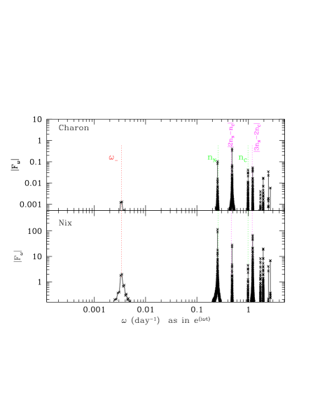
Figure 5.— Fourier decomposition of Charon & Nix’s eccentricity vector for the final state in Fig. 1. The Fourier amplitude $F_{\omega}=\int(e\cos{{\varpi}})\cos(\omega t)dt$ with orbital elements measured in Jacobi coordinates. The eccentricity of Charon is dominated by the 2:1 forcing term, while Nix by a combination of short term forcing. The peaks (indicated by $\omega_{-}$) are associated with the slowly decaying secular mode (NfC) which precesses at $\omega_{-}$ (eq. [42]). Their amplitude is a factor of $\sim 100$ below the total eccentricity.

In Figure 6, we “observe” the orbital state at the end of the simulation in the manner of Buie et al. (2006) by fitting Nix’s orbit to a Keplerian ellipse around a point mass at the barycenter with mass $M_{P}+M_{C}$ (where the value of $M_{P}+M_{C}$ is to be found by the fit). We also fit Charon’s orbit relative to Pluto with a Keplerian ellipse. We output the positions of Charon and Nix as functions of time from our numerical integrator. We then use the downhill simplex method (Press et al., 1992) to search fits for the set of 5 parameters: $e\cos{{\varpi}}$, $e\sin{{\varpi}}$, $a$, $M_{P}+M_{C}$ and $\tau$ (epoch of periapse passage). We find that the Keplerian-fit eccentricities are the secular parts of the total eccentricity, with the instantaneous values being much greater but averaged out in the fit. Therefore, somewhat counterintuitively, the Keplerian fit of Buie et al. (2006) provides a more useful diagnostic of Nix’s eccentricity than the 4-body fit of Tholen et al. (2007b).

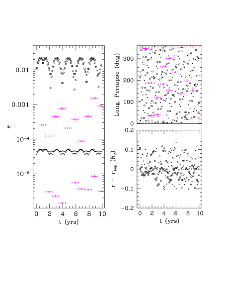
Figure 6.— Results of Charon & Nix orbital fitting for the final state in Fig. 1, insisting on Keplerian ellipses . We output data (points for Charon and open circles for Nix) once a month for 10 years, and do a Keplerian fit every 12 months (solid triangles for Charon and open triangles for Nix, error-bars in time-axis indicating span of Keplerian fit). Eccentricities are shown in the left panel: $e_{\rm Kep}$ fall well below the instantaneous values and are approximately the secular values (obtained from Fig. 5). The upper-right panel shows the value of ${{\varpi}}$, which varies on orbital timescales and are not captured by the Keplerian fits. The lower-right panel displays the fitting residuals measured by $r-r_{\rm kep}$ in unit of $R_{P}$. Charon’s residuals are magnified by a factor of $100$.

3.1.2 Charon’s eccentricity

Tholen et al. (2007b) report that $e_{C}=0.00348(4)$ when they do either a 4-body or a Keplerian fit, and that their earlier, much smaller value for $e_{C}$ (Buie et al., 2006) was incorrect. We find this large value of $e_{C}$ very puzzling. Our theory predicts that Charon’s eccentricity rapidly damps away by tides. More precisely, on the timescale $\tau_{C}\lesssim 10$ Myr, the CfN mode damps away. After this happens, Charon’s secular eccentricity in the NfC mode is $e_{C}\sim(M_{N}/M_{C})e_{N}$ as seen also in Figures 5-6. Thus Charon’s eccentricity should be much smaller than the Tholen et al. (2007b) value. It is highly implausible that Charon’s eccentricity was excited in the last $10$ Myr by some external event, such as flybys by passing Kuiper belt objects (Stern et al., 2003). In our view, the most plausible resolution of this puzzle is that the high eccentricity of Tholen et al. (2007b) is incorrect; perhaps inhomogeneities on the surface of Pluto or Charon are responsible for giving an apparent eccentricity. Future observations should help to resolve the puzzle.

3.2. Constraints on Nix’s Initial Orbit

Figure 7.— Trajectory of Nix’s orbit when tides damp Charon’s eccentricity. The top panel shows a numerical integration of the simplified model. The simulation is identical to the one shown in Figure 2, but here the eccentricity is plotted versus semimajor axis ratio. Similarly, the solid line in the bottom panel is the proper eccentricity from the N-body simulation shown in Figure 1, with the value of $a_{N}$ averaged over 100 days. The other curves in the lower panel are from N-body simulations that started with Nix both further in and further out, but also with $e_{N}=0.05$. The simplified model captures the essential behavior of the system but differs in detail, partly because the Laplace coefficients are taken to be constants, and partly because our disturbing function is only accurate to $O(\mu_{C})$. Nix’s current proper eccentricity is $\sim 0.002$ (Buie et al., 2006). The nominal location of the 4:1 resonance is shown as an arrow. Trajectories that have very low $e_{\rm N,sec}$ do not experience an appreciable jump when crossing this resonance (confirmed by further integration not shown here), while trajectories that have higher $e_{\rm sec}$ ($\geq 0.02$) do.

Let us consider the following scenario for explaining why Nix currently has a very low proper eccentricity, $e_{N}\sim 0.002$ (Buie et al., 2006): perhaps Nix formed with a high eccentricity at $a_{N}\lesssim 2.25a_{C}$, and then tidal evolution circularized its orbit as it was migrated to its current location, as in Figure 1. Note that Nix’s proper eccentricity at the end of that simulation is close to the Keplerian-fit value of Buie et al. (2006). The bottom panel of Figure 7 shows two additional N-body simulations with differing initial $a_{N}$. It illustrates that if Nix started inward of $\sim 2.25a_{C}$, its proper eccentricity is damped when it reaches its current location near the 4:1 resonance. But if it started beyond $2.25a_{C}$, it would have retained much of its initial eccentricity.

The difficulty with this scenario is that to have migrated Nix from inward of $2.25a_{C}$ to its current position, we require that $\tau_{C}\leq 2\times 10^{5}\,{\rm yrs}(\mu_{N}/0.00015)$ (Fig. 1), where $\mu_{N}\equiv M_{N}/M_{P}$. Even for $\mu_{N}\sim 0.00015$, this requires a tidal damping $>10$ times more efficient than the current estimate for the Pluto-Charon binary (Dobrovolskis et al., 1997). This seems difficult unless Charon is a molten sphere with large Love number $k_{2}$ (tidal distortion) and small $Q$ value. Moreover, it is a strange coincidence that Nix is so close to the 4:1 location today, since in our theory the outward migration of Nix does not pause at 4:1.

So unless the tidal dissipation time of Charon $\tau_{C}\lesssim 10^{5}$  yrs, Nix will have to be initially deposited at its present semimajor axis with proper eccentricity $0.002$, its current measured value. This places very stringent constraint for the formation scenario and rules out all but formation in a disc. In the latter case, the near 4:1 location is a result of migration in the disc (Shannon et al., in preparation).

Conversely, the fact that Nix could not have migrated further than from inward of the inner-most stable orbits ($a_{N}\sim 2.15a_{C}$) restricts $\tau_{C}$ to be $\geq 2\times 10^{5}$  yrs.

Appendix A Appendix A. Planetary Equations In Jacobi Coordinates

The Hamiltonian for Pluto, Charon, and Nix is

$$H={P_{P}^{2}\over 2M_{P}}+{P_{C}^{2}\over 2M_{C}}+{P_{N}^{2}\over 2M_{N}}-{{{G}}M_{P}M_{C}\over|\mbox{\boldmath$R$\unboldmath}_{P}-\mbox{\boldmath$R$\unboldmath}_{C}|}-{{{G}}M_{N}M_{C}\over|\mbox{\boldmath$R$\unboldmath}_{N}-\mbox{\boldmath$R$\unboldmath}_{C}|}-{{{G}}M_{N}M_{P}\over|\mbox{\boldmath$R$\unboldmath}_{N}-\mbox{\boldmath$R$\unboldmath}_{P}|}\ ,$$ (A1)

where $\mbox{\boldmath$R$\unboldmath}_{j}$ are position vectors from an arbitrary inertial origin, $\mbox{\boldmath$P$\unboldmath}_{j}=M_{j}d\mbox{\boldmath$R$\unboldmath}_{j}/dt$ are the conjugate momenta, and $M_{j}$ the masses. In Jacobi coordinates, Charon’s position is measured relative to Pluto’s, and Nix’s position is measured relative to the center-of-mass of the Charon-Pluto binary. We transform to Jacobi coordinates in two steps. First, we employ the generating function

$$F=(\mbox{\boldmath$R$\unboldmath}_{C}-\mbox{\boldmath$R$\unboldmath}_{P})\mbox{\boldmath$\cdot$\unboldmath}\mbox{\boldmath$p$\unboldmath}_{PC}+{M_{C}\mbox{\boldmath$R$\unboldmath}_{C}+M_{P}\mbox{\boldmath$R$\unboldmath}_{P}\over M_{C}+M_{P}}\mbox{\boldmath$\cdot$\unboldmath}\mbox{\boldmath$P$\unboldmath}_{PC}$$ (A2)

to switch the coordinates of the Pluto-Charon binary from $\mbox{\boldmath$R$\unboldmath}_{P},\mbox{\boldmath$R$\unboldmath}_{C},\mbox{\boldmath$P$\unboldmath}_{P},\mbox{\boldmath$P$\unboldmath}_{C}$ to the binary’s center-of-mass and its relative position vector,

$$\mbox{\boldmath$R$\unboldmath}_{PC} \equiv {M_{C}\mbox{\boldmath$R$\unboldmath}_{C}+M_{P}\mbox{\boldmath$R$\unboldmath}_{P}\over M_{C}+M_{P}}$$ (A3)

$$\mbox{\boldmath$r$\unboldmath}_{PC} \equiv \mbox{\boldmath$R$\unboldmath}_{C}-\mbox{\boldmath$R$\unboldmath}_{P}\ ,$$ (A4)

and their conjugate momenta ($\mbox{\boldmath$P$\unboldmath}_{PC},\mbox{\boldmath$p$\unboldmath}_{PC}$), yielding the new Hamiltonian

$$H={P_{PC}^{2}\over 2(M_{P}+M_{C})}+{p_{PC}^{2}\over 2M_{PC}}+{P_{N}^{2}\over 2M_{N}}-{{{G}}(M_{P}+M_{C})M_{PC}\over r_{PC}}-{{{G}}M_{N}M_{C}\over|\mbox{\boldmath$R$\unboldmath}_{N}-\mbox{\boldmath$R$\unboldmath}_{PC}-(1-\mu_{C})\mbox{\boldmath$r$\unboldmath}_{PC}|}-{{{G}}M_{N}M_{P}\over|\mbox{\boldmath$R$\unboldmath}_{N}-\mbox{\boldmath$R$\unboldmath}_{PC}+\mu_{C}\mbox{\boldmath$r$\unboldmath}_{PC}|}\ ,$$ (A5)

where

$$M_{PC}={M_{P}M_{C}\over M_{P}+M_{C}}$$ (A6)

is the reduced mass and

$$\mu_{C}={M_{C}\over M_{P}+M_{C}}\ .$$ (A7)

From Hamilton’s equation for $d{\mbox{\boldmath$R$\unboldmath}}_{PC}/dt,d{\mbox{\boldmath$r$\unboldmath}}_{PC}/dt$, we see that $\mbox{\boldmath$P$\unboldmath}_{PC}$ is the total momentum of the binary, and $\mbox{\boldmath$p$\unboldmath}_{PC}$ is the momentum of the relative orbit.

We complete the transformation to Jacobi coordinates with the generating function

$$F=\mbox{\boldmath$R$\unboldmath}_{PC}\mbox{\boldmath$\cdot$\unboldmath}\mbox{\boldmath$P$\unboldmath}_{PCN}+({\mbox{\boldmath$R$\unboldmath}_{N}-\mbox{\boldmath$R$\unboldmath}_{PC}})\mbox{\boldmath$\cdot$\unboldmath}\mbox{\boldmath$p$\unboldmath}_{N}$$ (A8)

which yields the new coordinate

$$\mbox{\boldmath$r$\unboldmath}_{N}\equiv\mbox{\boldmath$R$\unboldmath}_{N}-\mbox{\boldmath$R$\unboldmath}_{PC}\ ,$$ (A9)

as desired, as well as the new coordinate $\mbox{\boldmath$R$\unboldmath}_{PCN}\equiv\mbox{\boldmath$R$\unboldmath}_{PC}$; the conjugate momenta are $\mbox{\boldmath$p$\unboldmath}_{N}\equiv\mbox{\boldmath$P$\unboldmath}_{N}$ and the total center-of-mass momentum

$$\mbox{\boldmath$P$\unboldmath}_{PCN}\equiv\mbox{\boldmath$P$\unboldmath}_{PC}+\mbox{\boldmath$P$\unboldmath}_{N}\ .$$ (A10)

Since this is constant ($\mbox{\boldmath$R$\unboldmath}_{PCN}$ does not appear in the Hamiltonian), we may set it to zero. The Hamiltonian in Jacobi coordinates is

$$H(\mbox{\boldmath$p$\unboldmath}_{PC},\mbox{\boldmath$r$\unboldmath}_{PC};\mbox{\boldmath$p$\unboldmath}_{N},\mbox{\boldmath$r$\unboldmath}_{N})={p_{PC}^{2}\over 2M_{PC}}+{p_{N}^{2}\over 2M_{N}}\left(1+{M_{N}\over M_{P}+M_{C}}\right)$$ (A11)

$$-{{{G}}(M_{P}+M_{C})M_{PC}\over r_{PC}}-{{{G}}M_{N}M_{C}\over|\mbox{\boldmath$r$\unboldmath}_{N}-(1-\mu_{C})\mbox{\boldmath$r$\unboldmath}_{PC}|}-{{{G}}M_{N}M_{P}\over|\mbox{\boldmath$r$\unboldmath}_{N}+\mu_{C}\mbox{\boldmath$r$\unboldmath}_{PC}|}\ ,$$ (A12)

Thus far, our treatment has been exact. Henceforth, we drop the factor $M_{N}/(M_{P}+M_{C})$ in the second term above; although it is simple to retain it, we drop it for notational convenience. We choose units so that

$$G(M_{P}+M_{C})=1\ .$$ (A13)

By adding and subracting the term $-M_{N}/r_{N}$, the Hamiltonian may be written as

$$H(\mbox{\boldmath$p$\unboldmath}_{PC},\mbox{\boldmath$r$\unboldmath}_{PC};\mbox{\boldmath$p$\unboldmath}_{N},\mbox{\boldmath$r$\unboldmath}_{N})=H_{{\rm unp},PC}+H_{{\rm unp},N}+H_{\rm pert}\ ,$$ (A14)

where

$$H_{{\rm unp},PC} = {p_{PC}^{2}\over 2M_{PC}}-{M_{PC}\over r_{PC}}$$ (A15)

$$H_{{\rm unp},N} = {p_{N}^{2}\over 2M_{N}}-{M_{N}\over r_{N}}$$ (A16)

$$H_{\rm pert} = -{M_{N}M_{C}\over M_{P}+M_{C}}\left({1\over|\mbox{\boldmath$r$\unboldmath}_{N}-(1-\mu_{C})\mbox{\boldmath$r$\unboldmath}_{PC}|}-{1\over r_{N}}\right)-{M_{N}M_{P}\over M_{P}+M_{C}}\left({1\over|\mbox{\boldmath$r$\unboldmath}_{N}+\mu_{C}\mbox{\boldmath$r$\unboldmath}_{PC}|}-{1\over r_{N}}\right)\ ,$$ (A17)

Since we seek equations for the orbital elements, we transform variables to $\{a_{PC},\lambda_{PC},e_{PC},{{\varpi}}_{PC}\}$ and $\{a_{N},\lambda_{N},e_{N},{{\varpi}}_{N}\}$, defined in the usual way. (The mass of the cental body that enters into the definitions is $M_{P}+M_{C}$, both for Nix and for Pluto-Charon.) The equations of motion—Lagrange’s planetary equations—are given by Hamilton’s equations for canonical variables, which we may take to be the Poincaré variables , e.g. $\Lambda_{PC}\equiv M_{PC}\sqrt{a_{PC}},\Lambda_{N}\equiv M_{N}\sqrt{a_{N}}$, etc. (Murray & Dermott, 1999). It remains to express the Hamiltonian in terms of the orbital elements. The unperturbed terms are

$$H_{{\rm unp},PC} = -{M_{PC}\over 2a_{PC}}$$ (A18)

$$H_{{\rm unp},N} = -{M_{N}\over 2a_{N}}$$ (A19)

For the perturbed term, we resort to the usual Fourier expansion into a sum of cosine terms. Appendix B of Murray & Dermott (1999) tabulates the coefficients for the Fourier expansion of $1/|\mbox{\boldmath$r$\unboldmath}-\mbox{\boldmath$r^{\prime}$\unboldmath}|$ in terms of the orbital elements of one body at position $r$ and an exterior body at position $r^{\prime}$. (More precisely, that Appendix tabulates the direct part of the disturbing function, ${\cal{R}}_{D}\equiv a^{\prime}/|\mbox{\boldmath$r$\unboldmath}-\mbox{\boldmath$r^{\prime}$\unboldmath}|$.) Since equation (A17) consists of four terms of this form, we can easily extract the coefficients from Murray & Dermott (1999). These coefficients are functions of $\alpha$, the ratio of semi-major axes of the body at $r$ to the one at $r^{\prime}$. The coefficient for the term ${1/|\mbox{\boldmath$r$\unboldmath}_{N}-(1-\mu_{C})\mbox{\boldmath$r$\unboldmath}_{PC}|}$ should be evaluated at $\alpha=(1-\mu_{C})\alpha_{PC,N}$, where

$$\alpha_{PC,N}\equiv{a_{PC}\over a_{N}}\ ;$$ (A20)

similarly, the coefficient $1/r_{N}$ should be evaluated at $\alpha=0$, and that for $1/|\mbox{\boldmath$r$\unboldmath}_{N}+\mu_{C}\mbox{\boldmath$r$\unboldmath}_{PC}|$ at $\alpha=\mu_{C}\alpha_{PC,N}$. But there is an extra complication with the latter term, since $\mu_{C}\mbox{\boldmath$r$\unboldmath}_{PC}$ enters with a positive sign, instead of a negative one. To correct for this, one must set ${{\varpi}}_{PC}\rightarrow{{\varpi}}_{PC}+\pi$ and $\lambda_{PC}\rightarrow\lambda_{PC}+\pi$ in the argument of the cosine; equivalently, one must multiply by $-1$ if within the cosine argument the sum of the integer coefficients of ${{\varpi}}_{PC}$ and of $\lambda_{PC}$ give an odd number.

The procedure described above yields the equations of motion as precisely as desired when enough Fourier terms are retained in the disturbing function $H_{\rm pert}$ (aside from the factor $M_{N}/(M_{P}+M_{C})$ dropped from the Hamiltonian.) But for the purposes of this paper, it suffices to obtain coefficients that are incorrect by $\sim\mu_{C}\sim 10\%$. Therefore we expand $H_{\rm pert}$ to leading order in $\mu_{C}$. For each cosine term of the direct potential ${\cal R}_{D}\equiv a_{N}/|\mbox{\boldmath$r$\unboldmath}_{N}-\mbox{\boldmath$r$\unboldmath}_{PC}|$ of the form

$$\hat{\cal R}_{D}(\alpha_{PC,N})\cos\phi$$ (A21)

(suppressing the other arguments of $\hat{\cal R}_{D}$), we have

$$H_{\rm pert}=-\mu_{C}{M_{N}\over a_{N}}\hat{\cal R}\cos\phi\ ,$$ (A22)

where

$$\hat{\cal R}\equiv\hat{\cal R}_{D}(\alpha_{PC,N})-\hat{\cal R}_{D}(0)\pm\alpha_{PC,N}({D\hat{\cal R}_{D}})|_{\alpha=0}\ ,$$ (A23)

with $D\equiv d/d\alpha$ and $\pm\rightarrow+$ if the integer $d\phi/d\lambda_{PC}+d\phi/d{{\varpi}}_{PC}$ is even; otherwise $\pm\rightarrow-$.

Appendix B Appendix B. Effect of the 3:1 Resonance on the Secular Damping Rate

We solve the equations of motion for $z_{C}$ and $z_{N}$, including secular interactions, the 3:1 resonance, as well as tidal damping. The equations are given in §2.2, except here we discard the term $H_{2:1,CN}$; explicitly,

$${d\over dt}\left(\begin{array}[]{c}z_{{C}}\\ z_{N}\end{array}\right) = i{{\eta}}\left(\begin{array}[]{cc}\delta&-\beta\delta\\ -\beta&1\end{array}\right)\left(\begin{array}[]{c}z_{{C}}\\ z_{N}\end{array}\right)+i\nu\left(\begin{array}[]{cc}\upsilon\delta&-\chi\delta\\ -\chi&1\end{array}\right)\left(\begin{array}[]{c}z_{C}^{*}\\ z_{N}^{*}\end{array}\right)e^{i(3\lambda_{N}-\lambda_{C})}-\gamma_{C}\left(\begin{array}[]{c}z_{C}\\ 0\end{array}\right)\ ,$$ (B13)

where

$$\nu\equiv 2n_{N}\mu_{C}g_{7}\ ,\ \ \chi\equiv-{g_{6}\over 2g_{7}}\ ,\ \ \upsilon\equiv{g_{5}\over g_{7}}\ ,$$ (B14)

and the other quantities are the same as in equation (21). To solve these equations analytically, we take the semimajor axes to be fixed, setting

$$3\lambda_{N}-\lambda_{C}=n_{3:1}t$$ (B15)

where

$$n_{3:1}\equiv 3n_{N}-n_{C}$$ (B16)

is constant. We solve the equations perturbatively in the small parameter $\delta\ll 1$, adopting the same approach as in the paragraph above equation (44), i.e., we assume that $|z_{C}|\ll|z_{N}|$, which may be verified a postiori. To leading order in $|z_{C}|$,

$${dz_{N}\over dt}\simeq i\eta z_{N}+i\nu z_{N}^{*}e^{in_{3:1}t}\ .$$ (B17)

Replacing the $\simeq$ with $=$, this equation has solution

$$z_{N}=ke^{i(b+\eta)t}+{b\over\nu}k^{*}e^{i(n_{3:1}-b-\eta)t}\ ,$$ (B18)

where $k$ is the complex integration constant, and $b$ is either of the two roots of the quadratic equation that results from

$${b\over\nu}={\nu\over n_{3:1}-2\eta-b}\ .$$ (B19)

For definiteness, we choose the low-frequency root

$$b={n_{3:1}-2\eta\over 2}+\left(\left(n_{3:1}-2\eta\over 2\right)^{2}-\nu^{2}\right)^{1/2}\ .$$ (B20)

In the vicinity of Nix’s current semimajor axis $n_{3:1}<0$, implying that $b\simeq\nu^{2}/n_{3:1}$ to leading order in $|\eta/n_{3:1}|\sim 2\%$ and $|\nu/n_{3:1}|\sim 4\%$.

Inserting equation (B18) into the approximate equation for $z_{C}$,

$${dz_{C}\over dt}=-i\eta\beta\delta z_{N}-i\nu\chi\delta z_{N}^{*}e^{in_{3:1}t}-\gamma_{C}z_{N}$$ (B21)

yields

$$z_{C}=-\delta{\eta\beta+b\chi\over b+\eta-i\gamma_{C}}ke^{i(b+\eta)t}-\delta{\eta\beta b/\nu+\nu\chi\over n_{3:1}-b-\eta-i\gamma_{C}}k^{*}e^{i(n_{3:1}-b-\eta)t}\ ,$$ (B22)

discarding the homogeneous solution since it decays away after time $\sim\gamma_{C}^{-1}$.

Next, we rewrite the full equation for $z_{N}$ by inserting the approximate solution (B18) into equation (B13), with $k$ now time-varying, resulting in

$${dk\over dt}=-i{e^{-i(b+\eta)t}\over 1-b^{2}/\nu^{2}}\left[(\eta\beta+b\chi)z_{C}+(\eta\beta b/\nu+\nu\chi)z_{C}^{*}e^{in_{3:1}t}\right]$$ (B23)

Upon substitution of equation (B22), we arrive at

$${dk\over dt}=ipk+iqk^{*}e^{i(n_{3:1}-2b-2\eta)t}\ ,$$ (B24)

where

$$p\equiv{\delta\over 1-b^{2}/\nu^{2}}\left[{(\eta\beta+b\chi)^{2}\over b+\eta-i\gamma_{C}}+{(\eta\beta b/\nu+\nu\chi)^{2}\over n_{3:1}-b-\eta+i\gamma_{C}}\right]\$$ (B25)

and $q$ is a complex constant whose explicit form we do not give because we shall have no use for it. Equation (B24) has the same form as equation (B17), except that now the coefficients are complex. Its solution has the same form as equation (B18), except now multiplied by the prefactor $e^{-[{\rm Im}(p)]t}$. In conclusion, on timescales much longer than $1/\gamma_{C}$, $z_{N}$ slowly decays at the rate $\gamma_{3:1}\equiv{\rm Im}(p)$, or

$$\gamma_{3:1}={\delta\gamma_{C}\over 1-b^{2}/\nu^{2}}\left[\left({\eta\beta+b\chi\over b+\eta}\right)^{2}-\left({\eta\beta b/\nu+\nu\chi\over n_{3:1}-b-\eta}\right)^{2}\right]\ .$$ (B26)

This rate is plotted in Figure 3 relative to damping rate in the absence of the 3:1 forcing term.

Appendix C Appendix C: Hydra

Hydra’s evolution in the presence of Chaon is similar to Nix’s, but with some quantitative differences. Hydra’s purely secular damping rate relative to Nix’s is (eq. [30])

$${\gamma_{-H}\over\gamma_{-N}}={M_{H}\over M_{N}}{\sqrt{a_{H}}\over\sqrt{a_{N}}}{\beta_{H}^{2}\over\beta_{N}^{2}}=0.7{M_{H}\over M_{N}}\ ,$$ (C1)

where subscripts N and H are for Nix and Hydra, and the numerical expression is evaluated for Nix and Hydra at, respectively, the nominal 4:1 and 6:1 resonances with Charon. The 3:1 resonance has a relatively small effect on Hydra’s secular damping rate: from the extrapolation of Figure 3 to the nominal 6:1 resonance, it reduces $\gamma_{-H}$ by the factor $0.6$. Hydra’s forced eccentricity due to the 2:1 resonance with Charon is smaller than Nix’s by (eq. [61])

$$\left|{z_{H,2:1}\over z_{N,2:1}}\right|={g_{4,H}\over g_{4,N}}{n_{H}\over n_{N}}{n_{2:1,N}\over n_{2:1,H}}=0.2\ ,$$ (C2)

and its migration rate is reduced by (eq. [67])

$${\kappa_{H}\over\kappa_{N}}={M_{H}\sqrt{a_{H}}\over M_{N}\sqrt{a_{N}}}\left({g_{3,H}\over g_{3,N}}{n_{H}\over n_{N}}{n_{2:1,N}\over n_{2:1,H}}\right)^{2}=0.09{M_{H}\over M_{N}}$$ (C3)

It is also interesting to consider the interaction between Nix and Hydra. Hydra’s reported eccentricity based on a Keplerian fit differs from zero, $e_{H}=0.0052(11)$, and this might be due to the proximity of Nix and Hydra to their mutual 3:2 resonance. The 3:2 interaction energy between Nix and Hydra is

$$H_{3:2,NH}=-\mu_{N}{M_{H}\over 2a_{H}}\left(g_{a}z_{N}^{*}+g_{b}z_{H}^{*}\right)e^{i(3\lambda_{H}-2\lambda_{N})}+c.c.\ ,$$ (C4)

where $\mu_{N}\equiv M_{N}/(M_{C}+M_{P})$, $g_{a}=-(6+\alpha D)b_{1/2}^{3}/2=-2.03$, and $g_{b}=(5+\alpha D)b_{1/2}^{2}/2=2.48$, using $\alpha=(2/3)^{2/3}$ in the numerical expressions. Using the equation for Hydra’s eccentricity, it is simple to show that the 3:2 resonant term gives a forced eccentricity to Hydra equal to

$$z_{H,3:2}=\mu_{N}g_{b}{n_{H}\over 3n_{H}-2n_{N}-\eta_{H}}e^{i(3\lambda_{H}-2\lambda_{N})}.$$ (C5)

With the observationally derived values for $n_{H}$ and $n_{N}$ given in the Introduction, we find $|z_{H,3:2}|=0.003{\mu_{N}/10^{-4}}$, close to Hydra’s reported eccentricity. Since Nix and Hydra are close to 3:2 resonance, this eccentricity vector precesses at a slower rate than other resonantly forced eccentricity vectors (which precess at orbital timescales). It will show up in a Keplerian fit that covers many orbital periods. And we suggest that this likely explains the observed eccentricity of Hydra. Nix’s 3:2 forced eccentricity has a similar expression but scales with $\mu_{H}$. Tholen et al. (2007b) report a Hydra mass that is lower by a factor of 2 than Nix and encompasses zero. This is consistent with Nix’s lower measured eccentricity.

References

• Beust (2003) Beust, H. 2003, A&A, 400, 1129
• Buie et al. (2006) Buie, M. W., Grundy, W. M., Young, E. F., Young, L. A., & Stern, S. A. 2006, AJ, 132, 290
• Dobrovolskis et al. (1997) Dobrovolskis, A. R., Peale, S. J., & Harris, A. W. 1997, Dynamics of the Pluto-Charon Binary (Pluto and Charon), 159–+
• Goldreich (1963) Goldreich, R. 1963, MNRAS, 126, 257
• Lee & Peale (2006) Lee, M. H. & Peale, S. J. 2006, Icarus, 184, 573
• Levison & Duncan (1994) Levison, H. F. & Duncan, M. J. 1994, Icarus, 108, 18
• Murray & Dermott (1999) Murray, C. D. & Dermott, S. F. 1999, Solar system dynamics (Solar system dynamics by Murray, C. D., 1999)
• Ogilvie (2007) Ogilvie, G. I. 2007, MNRAS, 374, 131
• Press et al. (1992) Press, W. H., Teukolsky, S. A., Vetterling, W. T., & Flannery, B. P. 1992, Numerical recipes in FORTRAN. The art of scientific computing (Cambridge: University Press, —c1992, 2nd ed.)
• Stern et al. (2003) Stern, S. A., Bottke, W. F., & Levison, H. F. 2003, AJ, 125, 902
• Stern et al. (2006) Stern, S. A., Weaver, H. A., Steffl, A. J., Mutchler, M. J., Merline, W. J., Buie, M. W., Young, E. F., Young, L. A., & Spencer, J. R. 2006, Nature, 439, 946
• Tholen & Buie (1997) Tholen, D. J. & Buie, M. W. 1997, Icarus, 125, 245
• Tholen et al. (2007a) Tholen, D. J., Buie, M. W., & Grundy, W. M. 2007a, in AAS/Division for Planetary Sciences Meeting Abstracts, Vol. 39, AAS/Division for Planetary Sciences Meeting Abstracts, 62.09
• Tholen et al. (2007b) Tholen, D. J., Buie, M. W., Grundy, W. M., & Elliott, G. T. 2007b, ArXiv e-prints, 712
• Ward & Canup (2006) Ward, W. R. & Canup, R. M. 2006, Science, 313, 1107
• Weaver et al. (2006) Weaver, H. A., Stern, S. A., Mutchler, M. J., Steffl, A. J., Buie, M. W., Merline, W. J., Spencer, J. R., Young, E. F., & Young, L. A. 2006, Nature, 439, 943
• Wu & Goldreich (2002) Wu, Y. & Goldreich, P. 2002, ApJ, 564, 1024