Emission-Line Galaxies from the PEARS Hubble Ultra Deep Field: A 2-D Detection Method and First Results

Abstract

The Hubble Space Telescope (HST) Advanced Camera for Surveys (ACS) grism PEARS (Probing Evolution And Reionization Spectroscopically) survey provides a large dataset of low-resolution spectra from thousands of galaxies in the GOODS North and South fields. One important subset of objects in these data are emission-line galaxies (ELGs), and we have investigated several different methods aimed at systematically selecting these galaxies. Here we present a new methodology and results of a search for these ELGs in the PEARS observations of the Hubble Ultra Deep Field (HUDF) using a 2D detection method that utilizes the observation that many emission lines originate from clumpy knots within galaxies. This 2D line-finding method proves to be useful in detecting emission lines from compact knots within galaxies that might not otherwise be detected using more traditional 1D line-finding techniques. We find in total 96 emission lines in the HUDF, originating from 81 distinct “knots” within 63 individual galaxies. We find in general that [O iii] emitters are the most common, comprising 44% of the sample, and on average have high equivalent widths (70% of [O iii] emitters having rest-frame EW$>100$Å). There are 12 galaxies with multiple emitting knots–with different knots exhibiting varying flux values, suggesting that the differing star formation properties across a single galaxy can in general be probed at redshifts $\gtrsim 0.2-0.4$. The most prevalent morphologies are large face-on spirals and clumpy interacting systems, many being unique detections owing to the 2D method described here, thus highlighting the strength of this technique.

x

1. Introduction

It has long been known that galaxies display properties of their star formation through emission lines, and because of this, systematic studies of emission-line galaxies is an ongoing effort in order to investigate galaxies’ star formation–and thus evolution–throughout the history of the universe. Projects such as the KPNO International Spectroscopic Survey (KISS; Salzer et al. 2000) have investigated low-redshift emission-line galaxies’ properties (Salzer et al. 2001 & 2002). Spectroscopic studies of faint, intermediate-to-high redshift emission line galaxies have utilized large projects such as the CFRS (Lilly et al. 1995, Hammer et al. 1997), COSMOS (Capak et al. 2007, Lilly et al. 2007), and the DEEP1 and DEEP2 projects (Koo 1998, 2003; Willmer et al. 2006; Kirby et al. 2007). With the advantage of slitless grism spectroscopy from the Hubble Space Telescope’s (HST) Advanced Camera for Surveys (ACS), larger samples of faint objects — reaching to $i^{\prime}_{AB}\!\sim\!27.0$ mag — are now possible.

Many detailed studies have arisen from projects such as these. Earlier investigations have highlighted the importance of star formation bursts in interacting galaxies in general (Larson & Tinsley 1978), and subsequent studies have made use of emission-line fluxes to arrive at star formation rates (SFRs; Kennicutt 1998). In particular, H$\alpha$ emission has been used to derive SFRs and those results have been interpreted in the overall framework of galaxy evolution (Kennicutt 1983). Several studies have highlighted the importance of constraining the current SFR-density in the local universe using emission-line galaxies (Gallego et al. 1995, 2002; Lilly et al. 1995), while others have investigated the evolution of the SFR with redshift (Madau et al. 1998; Cowie et al. 1999). In the context of hierarchical merging, active star formation has long been regarded as a strong indicator of merging activity (Larson & Tinsley 1978), and recent studies have emphasized the evolutionary importance of merging galaxies and their role in AGN growth over cosmic time, both theoretically (di Matteo et al. 2005, Hopkins et al. 2005), as well as observationally (Straughn et al. 2006, Cohen et al. 2006). Studies of these types can be greatly enhanced by larger samples of faint star forming or emission- line galaxies at high redshift.

Slitless spectroscopy has been used often over the past several years to detect emission-line galaxies. In particular, HST’s Near Infrared Camera and Multi-Object Spectrometer (NICMOS) and Space Telescope Imaging Spectrograph (STIS) instruments have produced several surveys in which emission-line galaxies have been utilized to arrive at the H$\alpha$ line luminosity function and SFRs (e.g., Yan et al. 1999; HST NICMOS with the G141 grism), as well as the [O ii] luminosity function and star formation densities at intermediate redshifts (e.g., Teplitz et al. 2003; HST STIS with the G750L grism). The ACS G800L grism has also yielded very rich datasets, and the field of slitless spectroscopy with HST has culminated the past few years with the HUDF GRAPES (GRism ACS Program for Extragalactic Science; Pirzkal et al. 2004, Malhotra et al. 2005) project, and more recently with the PEARS (Probing Evolution And Reionization Spectroscopically) survey (Malhotra et al. 2007, in prep., Cohen et al. 2007, in prep.), which combined have yielded thousands of spectra over roughly half the area of the GOODS North and South fields including the HUDF to continuum fluxes of $i^{\prime}_{AB}\!\lesssim\!27$ mag. From the GRAPES data, studies of emission-line galaxies have been performed and a catalog has been compiled by Xu et al. (2007) using a 1D detection method described briefly below. Pirzkal et al. (2006) have performed analysis of GRAPES emission-line galaxies’ morphologies and evolution, highlighting the importance of studying these objects at $z\!\gtrsim\!1$. A key advantage of this project over similar ground-based studies is that the HST $i^{\prime}$-band sky brightness is $\sim\!3$ magnitudes darker than that from ground-based studies (Windhorst et al. 1994). With all the PEARS data analyzed, we anticipate increasing the sample of faint emission-line objects by a factor of 8–10 compared to the previous GRAPES project. In this methods-oriented paper we describe in detail several techniques aimed at detecting emission-line sources in the PEARS grism data and present our data and results for emission-line galaxies detected in the HUDF using a unique 2D line-finding method, which is shown to detect roughly twice the number of sources as 1D methods on the same data. A subsequent paper will contain the complete catalog of emission-line galaxies detected in the eight remaining PEARS fields, along with more detailed analysis of their properties, including quantitative morphological studies, star-formation rates, and line luminosity functions.

2. Data

The PEARS ACS grism survey data consist of eight ACS fields with three HST roll angles each (with limiting AB magnitude $i^{\prime}_{AB}\!\lesssim\!26.5$ mag; 20 HST orbits per field), plus the HUDF field with four roll angles (limiting AB magnitude $i^{\prime}_{AB}\!\lesssim\!27.5$ mag; 40 HST orbits total) taken with the ACS WFC G800L grism. The G800L grism yields low-resolution ($R\!\sim\!100$) optical spectroscopy between 6000-9500Å. Four PEARS fields were observed in the GOODS-N and five fields (including the HUDF) in the GOODS-S. A forthcoming data paper (Malhotra et al. 2007) will describe the PEARS project and data in detail. A description of the related GRAPES project can be found in Pirzkal et al. (2004): both the PEARS and GRAPES projects contain grism spectroscopy from the HUDF. Roll angles for the PEARS HUDF are $71^{\circ}$, $85^{\circ}$, $95^{\circ}$, and $200^{\circ}$. This paper will focus on emission-line galaxies detected in the HUDF, using the optimal of several methods described in Section 3. Preliminary source extraction produced a large catalog of PEARS objects in all nine fields with identifying numbers (Malhotra et al. 2007, in prep.). These PEARS IDs will be used in this paper.

3. Methods

This paper focuses on our efforts at identifying an efficient and robust method of detecting emission-line objects in the HST ACS PEARS grism data, particularly in objects with knotty morphologies and in continuum-dominated regions where lines might normally be missed. To this end, we have performed two separate, but related detections of PEARS HUDF emission-line galaxies that both rely on a unique 2D detection method, motivated by the observation that many emission lines originate from clumpy knots within galaxies (Meurer et al. 2007, Straughn et al. 2006b). Our results from these two 2D methods (hereafter “2D-A” and “2D-B”, described in detail below) will be compared to a separate method of detecting emission-line objects which relies on searching for lines in 1D extracted spectra from the HUDF PEARS data, as was also done for the GRAPES HUDF data (Xu et al. 2007).

The 2D detection procedure begins with pre-processing of the grism data, as described in detail in Meurer et al. (2007); here we give a brief description. Each image (both the grism and the direct $i^{\prime}$-band (F606W) image) was first “sharpened” by subtracting a 13x3 median smoothed version of the image from itself in order to remove most of the continuum from the grism spectra, leaving mostly compact features in the grism image. In this step, the long axis of the smoothing kernal is aligned with the dispersion axis of the grism. These are primarily emission lines in individual object spectra, as well as some residual image defects. This method was designed to detect lines in objects where continuum dominates and lines would otherwise be washed out. After this unsharp-masking stage, the next step is to mask out the images of the zero-order in the grism images. This is accomplished by matching compact sources found with the SExtractor program (Bertin & Arnouts 1996) in both the sharpened grism and direct images. This defines a linear transformation matrix which can be used to transform pixel coordinates from the direct to the grism frame, as well as scaling factor between the count rate in the direct image to that in the zero-order grism image (as described by Meurer et al. 2007). The geometric transformation is also used to derive a precise calibration of the row-offset between direct image sources and sources in first-order spectra. We determined that the transformation and row-offset are stable with HST pointing and roll-angle, and hence adopted the same values for all pointings. The mask is made by using the count-rate scaling to locate all the pixels in the direct image expected to be brighter than the noise floor in their zero order grism image. These are transformed to the grism coordinates, grown in size by three pixels to encompass the zero-order detection, and the resultant pixels are set to zero. Finally, SExtractor is used to catalog the masked filtered grism images in order to arrive at a list of emission-line source candidates, which is the input to both 2D emission-line source selection methods.

3.1. Method 2D-A: Cross-Correlation

The first of the 2D methods (“2D-A”) is a blind selection that relies on cross-correlation between the direct and grism sources, and is partially interactive (Meurer et al. 2007). Because of the interactive step, it is desirable to limit the amount of known contaminants that go into the algorithm. Since stellar sources often display a very strong continuum, sources with high SExtractor elongation parameters (ELONGATION$>2.5$) in the dispersed grism image were filtered from the catalogs to decrease the number of stellar sources. Sources that are very large or very small in the sharpened grism image are filtered out by only selecting sources with SExtractor parameter “FWHM” in the range of 1 to 10 pixels. This filtering reduces the number of sources that go into the 2D-A code approximately by half. Using these filtered catalogs, candidate emission lines are examined first in the grism image, and then the corresponding direct sources are located in the detection image. This is a semi-automated process in which lines in the grism image are displayed automatically, and the validity of each source is subsequently determined by eye. These potential emission-line sources are flagged as either: (1) a star; (2) a grism- or detection-image blemish (in which two cases the source is skipped); or (3) real, in which case the following is performed. For each “real” grism emission-line candidate, 5-pixel wide ribbons are extracted from both the grism and direct images, centered on the y-position (vertical in Fig. 1) of the source. The grism image ribbon is then collapsed down to a 1D spectrum. This spectrum is then cross-correlated with the direct image, and peaks are produced in the cross-correlation when knots within the direct image are detected that correspond to the grism image emission line. Typically only one peak is found in the cross-correlation yeilding a unique correspondence between line and emitting source. However, multiple peaks can occur due to the presence of multiple knots within galaxies or separate galaxies in the direct image ribbon. In those cases the corresponding source is selected manually. The correct choice is usually obvious from the location of the knot in the cross-dispersion direction (centered in the ribbon) or from the shape of the knot compared to the emission line in the filtered direct and grism images (Fig. 1; also cf. Fig. 1 of Meurer et al. 2007).

The 2D-A line-finding software produces an output list for each position angle with the detected emssion lines. In many instances, multiple knots with emission lines are detected in a single object. Catalogs are then matched to determine which emission-line sources are detected in multiple position angles. The final catalog for the 2D-A method was created by selecting sources which appear in at least two position angles (PAs).

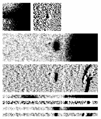
Figure 1.— Example of an object selected using Method 2D-A. Top panels show unfiltered grism image spectrum (left) and the same spectrum after median filtering (right). Middle two panels show direct image source both before and after the same median filtering. Bottom four panels show the 5-pixel wide “ribbons” (top two: grism; bottom two: direct) used in the correlation step to determine which direct image source the emission line originates from.

3.2. Method 2D-B: Triangulation

The second 2D technique (“2B-D”) uses triangulation. It starts with the same input catalog as above, but without any prior filtering and omission of sources based on their elongation and FWHM (however known M stars are removed from the catalogs beforehand). This method works because each source, and hence emission line, was observed at more than one PA on the sky, as is the case for our dataset. The ACS grism and ACS distortion are calibrated well enough so that one can map the position of emission-line sources detected in a distortion corrected grism image back onto the original distorted grism images, as well as onto true sky coordinates of RA and Dec (instead of simply using the detector x,y coordinates). When this is done for more than one PA, as shown in Figure 2, one can infer the location of the source of the emission line, which must necessarily lay somewhere along the direction of the grism dispersion. Once the source of the emission line has been inferred on the sky, we compute the wavelength of the detected emission line independently and along all PA dispersion directions (i.e. in all grism images where the line was detected). A true emission line source results in the same wavelength being derived (within an error that we set to 40Å, roughly one pixel), while a spurious detection leads to inconsistent results where the computed wavelength of a line is different when computed in different PAs. Since we have more than 2 observations taken in more than 2 PAs for this field, we actually used the method described above several times, using different pairs of PAs (i.e. $71^{\circ}$ vs $85^{\circ}$, $71^{\circ}$ vs 0$95^{\circ}$, etc..), as illustrated in Figure 2, looking for emission-line sources that produce consistent results for as many PA pairs as possible.

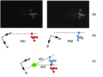
Figure 2.— The top two panels (a) show a series of emission lines observed at two different position angles (PA1 on the left, PA2 on the right). In both cases, the dispersion direction of the grism is nearly horizontal, as shown in (b), where we noted the true direction of North and East. Finally, the bottom diagram in (c) shows the remapping of the grism dispersion (dashed lines) onto the true sky (e.g. RA and Dec). As shown in (c), once remapped onto the sky, the two dispersion solutions intersect at a unique location (shown using the large circle). The latter is the inferred location of the source of the emission on the sky. We can then compute the expected wavelength of the emission line following the PA1 dispersion relation (d$\lambda$1) and following the PA2 dispersion relation PA2 (d$\lambda$2), and the two should agree (within the expected uncertainty).

3.3. Redshifts and line identifications

Three separate catalogs were used to obtain redshifts for the selected emission-line objects. First, photometric and spectroscopic redshift catalogs are from the GOODS-MUSIC sample (Grazian et al. 2006 and references therein). Spectro-photometric redshifts from Cohen et al. (2007) were used to supplement the MUSIC catalog when no MUSIC photometric redshift was available; this was the case for 16 objects. We also use Bayesian photometric redshifts (BPZs) from Coe et al. (2006) for the two objects (PEARS Objects 75753 & 79283) that had no spectroscopic redshifts, or MUSIC/Cohen photometric redshifts. Sixteen sources have 2 emission lines, allowing an immediate redshift determination using the ratio of line wavelengths which is invariant with redshift (note that given the grism resolution of $R\!\sim\!100$, H$\beta$ and the [O iii] doublet are usually blended). About a third of the sample ($\sim\!32$%) has spectroscopic redshifts and 95% have photometric redshifts. In total, three objects do not have any published redshift. Of these three, two (78237 Knot 1 & 89209) have 2 lines each, and thus a redshift was determined based on the wavelength ratios. The redshifts are used to help identify the emission lines in the grism spectra. Spectra with two distinct lines are in the minority (16 of 81 galaxy “knots”); most spectra have a single emission-line detection.

For objects with only one emission line, line identification then proceeds as follows. For the given object’s redshift (spectroscopic when available; photometric otherwise), potential wavelengths are calculated for H$\alpha$ , [O ii], [O iii], Ly${\alpha}$, [MgII], C iii], and C iv. An average spectro-photometric redshift error of $<\!\delta\!z\!>\!=\!0.04\!\times\!(\!1\!+\!z\!)$ (Ryan et al. 2007, Cohen et al. 2007, in prep., Coe et al. 2006) is used to calculate the likelihood of an identification as follows. Using the 4% photometric redshift error, a valid wavelength range for each potential line is calculated. Here, we also include the estimated 20Å wavelength calibration uncertainty (Pirzkal et al. 2004) intrinsic to the grism data. If the detected emission line candidate falls within the calculated wavelength range for any of the lines listed above, it is included in our final catalog. Once a confident line identification is made, we use the wavelength to recalculate the redshift; these new redshifts are given in Table 1. In comparing grism redshifts to spectroscopic redshifts, Meurer et al. (2007) arrive at a dispersion about unity of 0.007 for the 2D-detection method described here for secure line IDs (i.e., sources with two lines, or H$\alpha$ or [O ii] emitters, as these are typically the only plausible lines in the wavelength-range for that redshift). Line fluxes, rest-frame equivalent widths, and errors are then calculated by fitting gaussian profiles to the spectra using a non-linear least-squares fit to the given spectrum from five free parameters: the gaussian amplitude, central line wavelength, gaussian sigma, continuum flux level, and a linear term. Here we include a linear term in the fit to account for instances where the continuum is not flat. Line fluxes are averaged when the line is detected in two or more roll angles.

4. Results

The primary goal of this work is arrival at a robust and efficient technique to identify emission-line sources from the PEARS grism data that is as automated as possible. To this end, we have investigated in detail two versions of a 2D detection method as described in the previous section. Methods 2D-A and 2D-B produced 75 and 96 lines respectively, originating from multiple knots within galaxies. This is compared to 43 lines detected with the 1D method on the same data. Details of the results of these comparisons are discussed here, as well as a comparison to a catalog of emission-line galaxies generated from the related GRAPES grism data (Xu et al. 2007) using the 1D detection method.

4.1. ELG detections from three different methods

We summarize here in more detail detections resulting from three different methods outlined above. Note here the terminology used resulting from our 2D method: “lines” (sources detected in the grism image and hence distinct in position and wavelength), “sources” (which refer to individual clumps or knots within a galaxy), and “galaxies” (for example, one galaxy can contain three sources which each have two lines). The 1D line-finding method (as described in detail by Xu et al. 2007 for the GRAPES data) involves selection of emission lines from the 1D spectra generated by aXe  with visual confirmation. For the PEARS HUDF, 62 candidate lines were detected, 19 of which were flagged with a quality code indicating a contaminant or M-dwarf, resulting in a catalog of 43 PEARS galaxies. These remaining 43 galaxies are then compared to the catalogs generated by the two versions of our 2D line-finding method. Method 2D-A, the cross-correlation technique (§ 3.1), produced a final catalog of 75 lines, all of which originate from valid faint emission-line sources, since contaminants are thrown out in the user-interactive phase of the process described above. Individual PAs had 78, 114, 106, 77 detections in PAs $71^{\circ}$, $85^{\circ}$, $95^{\circ}$, and $200^{\circ}$ respectively; 75 of these were detected in at least 2 PAs. Method 2D-B, the triangulation technique (§ 3.2), produced a total of 96 lines. Method 2D-B also requires that an emission line be in more than one PA; in the final sample of 96 lines obtained with this Method, 12 were in two PAs, 38 were in three PAs, and 46 were in all four PAs.

Method 2D-A, described in detail in the previous section, requires some explanation of the results obtained since the software that produces the catalog is partially user-interactive. For PA085, two of the authors (ANS and GRM) ran the blind emission line-finding software on the data and compared results for completeness. It was found that there was a large (90%) overlap in final sources obtained between both users, suggesting that the method is robust in detecting secure emission-line sources, and user dependancies introduce relatively little bias. An investigation of the sources that were selected by one user and not the other shows several cases of multiple emission lines in knotty galaxies that often were offset from the other user’s detection by only a very small amount. There are a few cases of isolated galaxies where only one user detects a line. In general, the differences appear to be legitimate operator differences, and account for $<\!10$% of the detections. Those operator errors that are false detections are effectively weeded out by the requirement that the sources match in multiple PAs.

As described above, Method 2D-B (which uses traces in the grism image to determine the direct image emitting source) detects the most real lines in the PEARS data and discards spurious detections automatically. Because of this, it appears to be the most efficient and robust technique to detect emission-line sources in the grism data, and below we compare this method to the other two methods described here (Method 1D and Method 2D-A).

4.2. Comparison of Method 2D-B to Method 1D

First, we compare to the 1D method used on the same PEARS data. Here we find that Method 2D-B detects $1.9\!\times$ as many sources for this field. Overall, the overlap between the two methods is 72%, with the 1D method detecting 12 unique sources and the 2D method detecting 50 unique sources. We note here that the input to the 1D method is the SExtractor catalog of entire galaxies, in contrast to our SExtractor catalog of individual galaxy knots. Thus in regard to the 1D method, the emission lines are diluted by the continuum and the equivalent width goes down below the detection limit. An inspection of the initial 2D-generated input files in comparison to these 12 1D-detected but 2D-undetected sources shows several aspects of interest. First, the majority of these 12 1D-detected sources are clustered along the edges of the field, with only 3 of them extending inwards more than 700 pixels (or 1/5 the width of the image). This suggests—and was confirmed on more detailed inspection—that many times the object in question is undetected in at least one PA (sometimes up to three PAs), and would thus not make it into the final catalog produced by the 2D-B method. Second, we notice that only in a very few cases are there any SExtractor detections located along the dispersion direction for any given 1D-only detected object. This shows that these sources were not in the input SExtractor catalogs because they were below our 2D-detection limit, thus explaining the absence from our final 2D-B ELG catalog. Figure 3 shows an estimate of signal-to-noise for these 1D-detected objects, and indicates that the 1D-detected objects that were missed by the 2D method were in general lower S/N and likely below our detection limit imposed in the initial grism emission-line catalog selection.

Figures 4- 6 show some examples of 2D-detected galaxies with several emitting knots. These composite images were created using the HUDF F435W ($B$), F606W ($V$), F775W($i^{\prime}$), and F850LP ($z^{\prime}$) data. Objects 70314 and 78491 were not detected using the 1D technique. This is likely due to continuum flux dominating the spectrum, an effect which was mitigated in our technique by the sharpening process (see Section 4.6 for a full discussion of these objects). Therefore, in general, it is shown that the overlap between Method 1D and Method 2D-B is large, and the 1D objects missed by the 2D-B Method are due to our imposed detection threshhold. In total, the 2D Method finds almost twice as many sources.

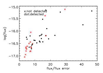
Figure 3.— Signal to noise estimates of PEARS objects detected with the 1D Method. Black dots are 1D-detected objects that are also detected with our 2D-B Method; red x’s are 1D-detected objects that are missed by the 2D-B Method. Fluxes are from Xu et al. . In general, objects missed by Method 2D-B are lower S/N, clustered below S/N$\sim\!8\!-\!10$.

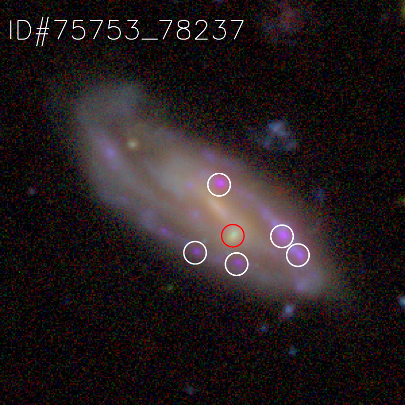
Figure 4.— PEARS Objects 75753 & 78237. Stamp is 9” across; this galaxy has a redshift $z=0.339$. These were extracted as two sources but are part of the same galaxy. The knot indicated by the red circle is likely an interloper with an undetermined redshift. The other five knots all contain H$\alpha$ and/or [O iii] emission; flux values are given in Table 1. This composite image (as well as Figures 5 & 6) was constructed using the HUDF $B,V,i^{\prime},z^{\prime}$ data.

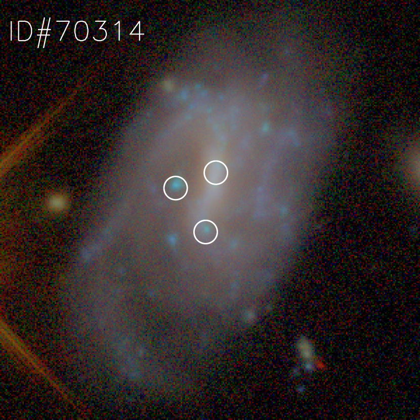
Figure 5.— PEARS Object 70314. Stamp is 9” across; this galaxy has a redshift $z=0.144$. All three knots have H$\alpha$ emission. The line from the nuclear region of the galaxy has an equivalent width $\sim$4$\times$ smaller than that from the other two knots. This result highlights the strength of the 2-D Method utilized here: this galaxy has no detected lines using the 1-D Method in either the PEARS or GRAPES data, presumably because the line flux was overwhelmed by continuum flux when light from the entire galaxy was extracted. However, narrowing in on individual knots allows us to see the line emission.

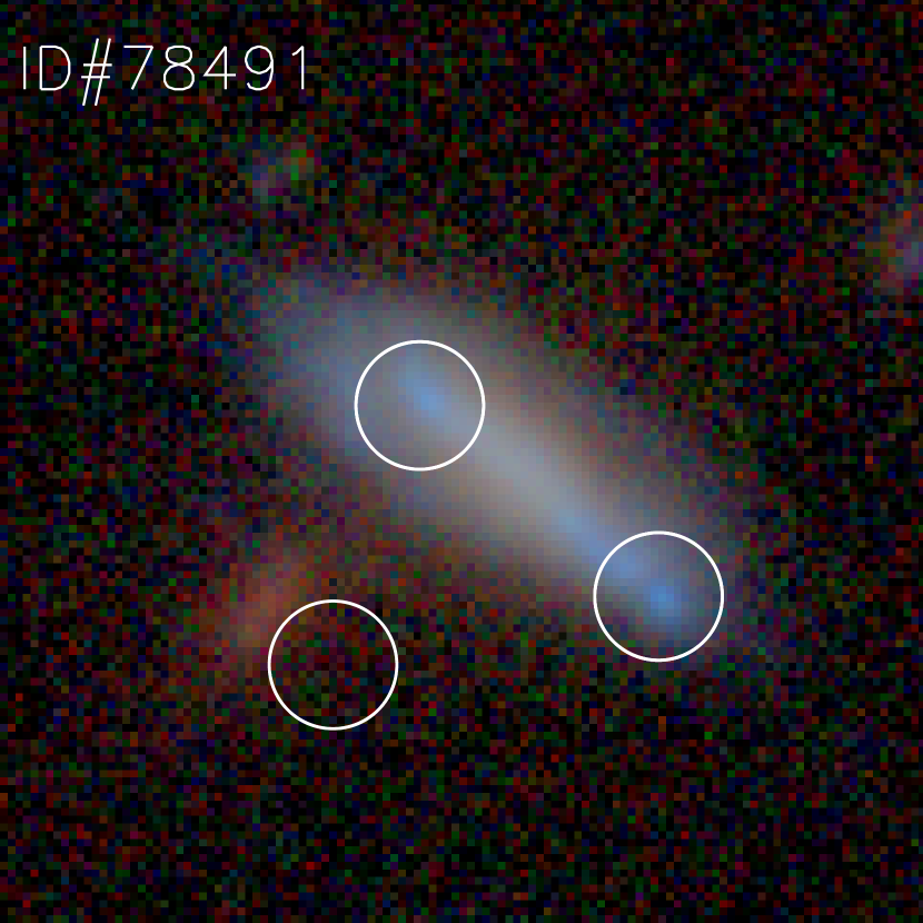
Figure 6.— PEARS Object 78491. Stamp is 3.6” across; this galaxy has a redshift $z=0.234$. The two blue knots on the ends of the galaxy each have H$\alpha$ and [O iii] emission; the knot on the left-hand side of the galaxy has stronger [O iii] flux by a factor of $\sim\!2$ and the right-hand side knot has slightly stronger H$\alpha$ flux. The third circled “knot” is clearly not part of this PEARS galaxy, although it is emitting a very strong line ($EW\!=\!237.0$Å) at $\lambda\!=\!7143$Å. No redshift is available for this object, however, so line identification is not possible.

4.3. Comparison of Method 2D-B to Method 2D-A

Given that Method 2D-B was developed in conjunction with Method 2D-A, a comparison between these two methods is warranted as well. As described above, both methods have identical input catalogs for each PA, with the exception that the input to method 2D-A was pared down to avoid selection of undesired objects (i.e. stars) in the user-interaction phase of the analysis. Comparison of Method 2D-B to Method 2D-A shows that all but 2 sources detected by Method 2D-A were also detected by Method 2D-B, an overlap of 96%. Additionally, the level of human interaction is greatly reduced in Method 2D-B, making it both more efficient and reliable.

4.4. Comparison of Method 2D-B to GRAPES catalog

Although the GRAPES project (Pirzkal et al. 2004, Malhotra et al. 2005) involves a different dataset than the one used for the present work, a comparison of our results to the previous GRAPES ELG catalog in Xu et al. (2007) is explored here since the data are for approximately the same field. Figure 7 gives a graphical comparison of the PEARS and GRAPES fields centered on the HUDF. The process used to arrive at the GRAPES ELG catalog is the same as “Method 1D” described above, with some manual additions (approximately 10%) of objects after visual examination of all the individual spectra as described in that paper. The first difference in the two datasets is that the Xu et al. (2007) ELG catalog utilized the GRAPES data (40 HST orbits) plus one epoch of preexisting ACS grism HUDF data, increasing the observed grism exposure time by about one-fifth (Pirzkal et al. 2004) and also increasing the overall combined area observed. Second, since the fields are not exactly overlapping, there are some GRAPES ELG objects that are not in the PEARS fields and vice versa. Given these factors, the comparison is not as straightforward as, e.g., the comparison to the 1D Method applied to the identical PEARS data, as described above. However, when doing the comparison, we find that 61% of the 2D-B detected sources are in the GRAPES catalog, with 37 unique lines appearing in the 2D-B catalog only. Of the 39% of GRAPES sources unique to the GRAPES catalog, many are found to exist outside of the PEARS observing area. Specifically, 44%, 34%, 34%, and 27% of the 2D-B-undetected GRAPES sources fall outside the four PEARS roll angles $71^{\circ}$, $85^{\circ}$, $95^{\circ}$, and $200^{\circ}$ respectively. In total, there are 35, 41, 41, 45 sources in the four respective PEARS PAs that are not detected with Method 2D-B. The sources that were detected with the 1D Method from GRAPES but were missed by 2D-B in general were missed for the same reason as with Method 1D used on the PEARS data (as described in Sec. 4.2): those missed were below our S/N threshhold required for Method 2D-B (Fig. 3). In particular, the missed objects generally have S/N$\sim\!2\!-\!3$, while most of our objects detected in GRAPES generally have higher S/N values. We thus conclude that this is the same effect as was seen when comparing to Method 1D for the PEARS data. This is expected given our detection limit which serves to greatly increase the reliability of our 2D detection method.

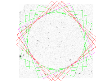
Figure 7.— The four PEARS HUDF pointings are shown in green, as well as the four GRAPES shown in red (plus one archival ACS grism field uses in the GRAPES study shown in magenta; see Sec. 2). All PEARS and GRAPES fields are centered on the HUDF. Eight additional PEARS fields will be analyzed in a future study: four fields in the GOODS-N and four more in the GOODS-S.

4.5. ELG catalog and statistics

Our final catalog of PEARS HUDF emission-line objects, derived from the most efficient method investigated here—Method 2D-B—is given in Table 1. In total, 96 distinct lines were detected in 81 galaxy sources or “knots” in 63 PEARS galaxies. Examples of galaxies with several emitting knots are shown in Figures 4– 6, demonstrating the strength of the 2D Method as compared to the 1D Method. In addition, Figure 8 shows how the 2D Method is able to detect lines in galaxies that were undetected by the 1D Method due to strong continuum overwhelming the emission lines. The percentages of identified lines are as follows: 34% are H$\alpha$ , 14% are [O ii], and 44% are [O iii], with 3% accounting for other less common lines ( MgII, C iii], and C iv). Our catalog includes 39 new spectroscopic redshifts for galaxies that are on average fainter than the standard magnitude limited redshift survey ($z^{\prime}_{AB}\!=\!23.5$ mag for ground-based GOODS spectroscopic redshifts; Elbaz et al. 2007). The faintest ELG has a continuum $i^{\prime}_{AB}\!=\!27.4$ mag, and the average continuum magnitudes of H$\alpha$ , [O ii], and [O iii] emitting galaxies are $i^{\prime}_{AB}\!=\!21.9$, $24.1$, and $23.6$ mag respectively. The magnitude distribution of the sample is given in Figure 9.

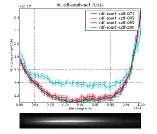
(a) 1D Extraction

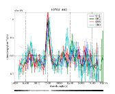
(b) 2D Extraction

Figure 8.— (a): 1D extraction of PEARS Object 70314 (entire galaxy; see also Figure 12). Top panel shows the 1D spectrum from 1D extraction; bottom panel shows the 2D spectrum of this object. Top-right inset gives labels for the four HST roll angles used in this dataset ($71^{\circ}$, $85^{\circ}$, $95^{\circ}$, and $200^{\circ}$). Scale of y-axis is in units of $10^{-17}$ (b): 2D extraction of Knot # 2 in the same galaxy. Panels and inset are the same as in (a). Here the y-axis scales in $10^{-19}$. This is an example of the success of the 2D extraction method: no lines are detected when the 1D extraction of the entire galaxy is performed. However, the 2D extraction of three separate emitting knots in this galaxy reveals strong emission lines in the spectra of all three knots.

Figure 9.— Histogram of $i^{\prime}$-band magnitudes of all PEARS HUDF emission-line objects, showing a peak in the distribution around $i^{\prime}_{AB}\!\simeq\!24$ mag. The PEARS HUDF continuum detection limit is $i^{\prime}_{AB}\!=\!27.4$ mag (Malhotra et al. 2007, in prep.).

The faintest line flux is $5.0\!\times\!10^{-18}$ ergs cm^-2s^-1, with the average line flux being $3.9\!\times\!10^{-17}$ ergs cm^-2s^-1. The [O iii] emitters have on average high equivalent widths, with 70% of them having $EW\!>\!100$Å. The line flux distribution for all sources is given in Figure 10, while Figure 11 gives the line flux distributions for the individual lines.

Figure 10.— Line flux distribution of all lines detected with Method 2D-B, in units of $10^{-18}ergscm^{-2}s^{-1}$.

Figure 11.— Individual flux distributions of H$\alpha$ , [O iii], and [O ii] lines. The distributions peak at $\sim$$2.5\times 10^{-17}$ ergs cm^-2s^-1 for H$\alpha$ and [O iii], and near $5.0\times 10^{-18}$ ergs cm^-2s^-1 for [O ii].

An interesting potential trend appears in Figure 12, which shows the equivalent width of PEARS HUDF [O ii] lines as a function of redshift as compared to nearby galaxies from Jansen et al. (2000) and intermediate redshift galaxies from the CFRS sample (Hammer et al. 1997). It is clear that the EW of the PEARS [O ii] sources are extremely high compared to local samples–especially above $z\sim 1.1$. Here we note that grism selection of [O ii] emitting regions systematically selects higher-EW objects in the [O ii] redshift range probed by the grism (which could be due to the smaller HST PSF including less continuum from the surrounding area of the knot, thus raising the observed EW; see the sensitivity limit plotted in Fig. 12). Hence the fact that the average EW is higher than local galaxies is not surprising. However, the discovery of [O ii] emitters with EW$>100$Å is interesting. These are exceedingly rare in the local universe (Jansen et al. 2000), and here we only see them at the highest redshifts ($z>1.1$). As shown in Fig. 12 they are also known from previous ground-based surveys (CFRS; Hammer et al. 1997), and appear to be more common with increasing $z$ (Cowie et al. 1996). Sources with similar (and higher) EW([O ii]) were also reported in previously published HST slitless observations (Meurer et al. 2007; Teplitz et al. 2003). Teplitz et al. (2003), in particular, find a high incidence of EW $\gtrsim$100Å [O ii] emitters at z$\lesssim$0.5, while noting that at high redshifts, lower EW lines might have been missed in comparative surveys. While statistics are low presently, and thus no definite statement can be made concerning this trend, several possible explanations of its origin exist. For example, strong evolution of galaxies’ star formation properties with redshift would cause this occurance of very high [O ii] EW at high redshift. Additionally, lower extinction between the sources of ionizing radiation and the gas would produce higher EW values. However, this phenomenon could also be caused by cosmic variance; the comoving volume of the PEARS HUDF is clearly much less than the local sample and the 0.2 $\lesssim$z $\lesssim$1.0 sample, and this effect could influence results presented here. As an example of this effect, Takahashi et al. (2007) found that [O ii] emitting star-forming galaxies in the COSMOS field show clustering tendencies at redshifts z$\gtrsim$1.2. We anticipate a better study of this phenomenon when the other eight PEARS fields are analyzed and simulations of the data are available to aid in sorting out various selection effects.

Figure 12.— Rest-frame equivalent width as a function of redshift for [OII] emitters. Stars are PEARS HUDF [O ii] emitters, filled dots are from Jansen et al. (2000) and small dots are from the Canada-France Redshift Survey (Hammer et al. 1997). For our sample, [O ii] can be detected in the redshift range $0.6\!\lesssim\!z\!\lesssim\!1.5$ given the grism range 6000-9500Å. Approximate PEARS selection limit is given by solid line.

The redshift distribution of these ELGs is shown in Fig. 13, with the majority of redshifts lying between $z\!=\!0$ and $z\!=\!1.5$ and the peak occuring around $z\!\sim\!0.5$. Since the identified lines—which are only observable at the redshifts in the plot—are generally the strongest lines in star-forming galaxies, this explains why the emission-line N(z) peaks at a lower $z_{max}$ than the field galaxy photometric redshift distribution which peaks at $z\!\sim\!1\!-\!1.5$. This is thus in part an artifact of the ACS grism selection function (see Malhotra et al. 2005).

Figure 13.— Redshift distribution for PEARS ELGs showing peak of distribution around z$\sim$0.5. Given the grism properties (sensitive from 6000Å to 9500Å), the H$\alpha$ line is observable from 0$\lesssim$z$\lesssim$0.4; [O iii] from 0.1$\lesssim$z$\lesssim$1.1, and [O ii] from 0.4$\lesssim$z$\lesssim$1.5. The one object at higher redshift in this figure is the AGN (C iv  C iii] emitter) at $z=3.17$. Because the identified lines are only available at these particular redshifts (and are generally the strongest lines in star-forming galaxies), the emission-line N(z) peaks at a lower $z_{max}$ than the field galaxy photometric redshift distribution which peaks at $z\sim 1-1.5$ (Ryan et al. 2007, Cohen et al. 2007, in prep.).

A qualitative look at the morphologies of the emission-line galaxies (in $B,V,i^{\prime},z^{\prime}$; see Fig. 4-6) suggests that the majority of these objects are clumpy, knotty galaxies that have distinct emitting regions of presumably active star formation. In particular, we find many face-on knotty spirals, as well as clumpy interacting systems with regions of enhanced star formation that were missed with the 1D Method. A subsequent paper will investigate the emission-line galaxies’ morphologies in a quantitative manner, including the results of the selection for the entire PEARS dataset in addition to these HUDF ELGs.

4.6. Line luminosities of PEARS galaxies: Comparison to nearby galaxies

From our sample, there are 33 H$\alpha$ and 13 [O ii] emission regions from galaxies at average redshifts of $z\!\sim\!0.26$ and $z\!\sim\!1.05$ respectively. Here we discuss the properties of these objects in terms of their line luminosities in comparison to local samples from Kennicutt et al. (1989) and Zaritsky et al. (1994). Figure 14 gives the luminosity histogram of PEARS HUDF H$\alpha$ emitters (solid line) with the slope of the local HII region H$\alpha$ distribution from Kennicutt et al. (1989) as a dot-dashed line. We have also plotted the best fit line of the bright end of our distribution with a dashed line. Here we see that the grism observations do not detect some of the fainter emission, as is expected; however, we do detect brighter sources, lending to the shallower slope. We note here that this effect is not due to spatial resolution: at $z\!\sim\!0.3$, each pixel is $\!\sim\!130$ parsecs, and Kennicutt et al. (1989) show that there is almost no difference in the luminosity histograms when degrading the spatial resolution from 30 to 300 parsecs.

When we investigate line luminosites of individual knots from the nearby Zaritsky et al. (1994) sample (Figure 15), we see two distinct distributions, with the high redshift PEARS [O ii] emitters having systematically higher luminosities. A selection effect exists here, as we can only detect the brightest sources at high redshift (detection limit of $log(L([O\,{\sc ii}])\/\mbox{L${}_{\odot}$})\sim 6.3$ in Fig. 15). The fact that we miss the lower luminosity [O ii] emitters in this dataset does not negate the fact that we do see very high luminosity sources at this redshift in the grism data (see also discussion of high-EW [O ii]sources in previous section).

Figure 14.— Distribution of H$\alpha$ line luminosities of the PEARS galaxies (median redshift of z$\sim$0.26), with the local Kennicutt et al. (1989) sample’s bright-end slope plotted as a power-law (dot-dashed line; a=-3.3). The PEARS sample slope differs from the local one (a=-0.58); we detect more bright H$\alpha$ emitting regions in the grism data.

Figure 15.— Distribution of [O ii] line luminosities of the PEARS galaxies (solid line multiplied by a factor of 8; median redshift of $<\!z\!>\!\sim\!1.05$) and of HII regions within nearby galaxies from Zaritsky et al. (1994; dashed line). The grism observations are well-suited to detect high-redshift sources with very high [O ii] luminosities. Note here our detection limit (shown in Fig. 12)

4.7. Galaxies with multiple emitting knots

Individual HII regions in nearby galaxies have been studied for some time (Shields 1974; McCall, Rybski, & Shields 1985, Zaritsky, Kennicutt, & Huchra 1994, etc.), and it is well known that star formation properties vary in local galaxies from one star forming region to another. For example, Kennicutt, Edgar, & Hodge (1989) find that the luminosity function of HII regions in spiral arms and interarm regions differ greatly. Zaritsky, Kennicutt, & Huchra (1994) also find measurable differences in line luminosities of individual star forming regions in nearby galaxies. Gordon et al. (2004) investigate in detail the variations of H$\alpha$ (as well as UV and infrared) star formation rates in the many star-forming regions of M81. Additionally, star-forming clumps in the interacting system IC2163 & NGC2207 are studied by Elmegreen et al. (2006). However, investigation of individual emitting regions in high-redshift galaxies has not been explored as extensively. Studies of this kind focus on physical processes occuring within the galaxy, and comparisons of the high redshift sample to local galaxies help to sort out possible evolutionary effects. As noted above, 12 of our 63 2D-selected emission-line galaxies ($\sim\!20$%) have multiple emitting knots, many of which display multiple lines. These galaxies lie in the redshift range of $0.12\lesssim$z$\lesssim 0.44$, the faintest of which has a continuum magnitude of $i^{\prime}_{AB}=23.64$ mag. Here we focus on several of these PEARS galaxies that have spatially distinct emitting knots.

PEARS Object # 75753/78237 (SExtractor extracted this object as two separate objects, but visual inspection shows that the two selected regions are part of the same galaxy) has six separate emitting regions, four of which have both H$\alpha$ and [O iii] emission (one knot containing only [O iii] emission). This object is shown in Figure 4. In the three knots (which are in 75753) that have both lines, the [O iii] flux is approximately 2$\times$ the H$\alpha$ flux (which indicates high excitation, which often means low metallicity). The other knot (in 78237) that has both lines has roughly equal flux in both H$\alpha$ and [O iii]. The H$\alpha$ flux differs by a factor of up to $\sim$3.5, suggesting a variation in star formation rate across the complex structure of this galaxy. The knot indicated by the red circle in Figure 11 has an unidentified line with a wavelength inconsistent with the others present in this source and with no viable alternative line at this redshift ($\lambda_{obs}$=7872Å ;$\lambda_{RF}$=5875Å if the line originated from this galaxy). We also note that this object has a slightly different color than the rest of the nuclear region of the galaxy. Given these factors, we conclude that the “knot” within the red circle is an interloper at an undetermined redshift, whose emission line is present in the spectrum of Object 75753/78237.

PEARS Objects 70314 and 78491 each have three emitting knots (Figures  5 and 6 respectively). Object # 70314’s three knots all have H$\alpha$ emission, with two knots having roughly equal H$\alpha$ flux and equivalent widths, and the other knot having lower flux and equivalent width values by a factor of $\sim$4. This galaxy is a good example of the success of the 2D line-finding method: the lines in this galaxy—with its multiple blue star-forming regions—were not detected with the 1D method in either the PEARS or GRAPES data, because the line flux was washed out by the continuum flux from the galaxy’s core (see also Fig. 8). Following this same line of reasoning, the weakest line of the three is the one originating from the nucleus of the galaxy # 70314 (Fig. 5). The lines stand out more when extracted solely from the emitting knots instead of the entire galaxy. All of the lines associated with Object # 78491 have equivalent widths $\gtrsim\!100$ Å (Table 1). Two of the knots contain both H$\alpha$ and [O iii], and originate from blue star-forming regions on the ends of the galaxy disk (Fig. 6). The third “knot” associated with this PEARS ID appears to be another object and has a strong line ($EW\!=\!237.0$ Å) that remains unidentified due to lack of redshift for this particular object ($\lambda_{obs}$=7143Å ;$\lambda_{RF}$=5788 for $z$=0.234, the redshift of Object # 78491) .

PEARS Objects 63307, 70407, 75547, 77558, 79283, 79483, 81944, and 88580 all have two emitting knots. The properties of these galaxies are given in Table 1. Object # 81944 has strong H$\alpha$ and [O iii] emission from one of its knots and a relatively weak H$\alpha$ line in the other (with an equivalent width of $\sim\!4.5$ times lower). There are other cases (IDs 79283 and 88580, for example; $z\!=\!0.23$ and $z\!=\!0.269$ respectively) where line flux differs by a factor of 2 or more across a single galaxy. This indicates that the star formation properties of these objects differ across the galaxy itself, and that this effect in general can be probed at redshifts $z\!\gtrsim\!0.2$.

We also note here that five of the twelve galaxies with multiple emitting knots did not have detected lines in the deeper GRAPES+1 ACS field data (described above; Sec. 4.4). Among the galaxies that were detected in GRAPES, the PEARS-detected lines’ equivalent widths were higher in every case by on average a factor of$\sim\!4\!\times$. This again underscores the strength of the 2D method, which serves to isolate line emission from individual knots, such that continuum emission from the rest of the galaxy does not dominate the spectrum.

Given the subset of PEARS HUDF galaxies that exhibit multiple emitting knots, we expect to have a statistically significant sample of these objects once analysis of the entire PEARS dataset is completed. This should allow an in-depth study of localized star formation at galaxies up to $z\!\sim\!0.4\!-\!0.5$.

5. Summary and Future Work

In summary, it is clear that although each method has some unique detections, Method 2D-B (triangulation) in general is quite efficient at detecting emission-line sources in the PEARS grism data, especially for objects with knotty structures or strong continuum that remain undetected with the 1D method. The reason for this advantage is that the 1D method gives line flux integrated over the whole galaxy, while the 2D method gives line flux from the emitting region only (i.e. galaxy knots). Triangulation requires observations obtained at multiple roll angle, and hence may not be suitable to all grism datasets. Method 2D-A (cross-correlation) can be used with ACS grism data obtained at one PA (Meurer et al. 2007), but is not fully automated and may produce false identification of emitting sources in confused regions such as in extended galaxies. The triangulation method will be utilized in future studies of the remaining eight PEARS fields. Given the sample of 81 distinct emitting regions, we expect a total sample of $\sim\!600\!-\!700$ ELGs to continuum $i^{\prime}_{AB}\!\lesssim\!26.5$ mag from the combined depth and area of the PEARS North and South fields. From this larger statistical sample, two primary investigations will follow. First, we will derive line luminosities, which should allow us to constrain the luminosity function for H$\alpha$ , [O ii], and [O iii], going fainter and to higher redshifts than previous studies. Secondly, we will use the luminosities and equivalent widths to estimate the change in the cosmic star formation rate, again utilizing the depth and quantity of the PEARS data. In order to account for dust attenuation, we plan to estimate an average correction for the different redshift bins in the survey following previous authors. For example, Davoodi et al. (2007) calculated estimates for a sample of 1113 SDSS galaxies in the SWIRE survey (using the extinction law from Calzetti et al. (1994)). Kewley et al. (2004) used the redding curve of Cardelli, Clayton, & Mathis (1989). Additionally, Thompson et al. (2006) give examples of extinction and surface brightness dimming corrections to star formation rates for HUDF galaxies with redshifts 1-6. Pixel-to-pixel SED decompositions of HUDF galaxies are currently being performed by Ryan et al. (2008, in prep.) and will also provide estimates for the effects of dust over a large redshift range. In addition to these two primary goals, we will also investigate in further detail the possible evolution of [O ii] equivalent width and luminosity with redshift (Figs. 12 & 15). The $z=0-1.5$ range is where the SFR density shows its strongest evolution. Use of the grism to isolate the strongest EW sources in this redshift range, combined with deep HST imaging, will prove to be an excellent way to select galaxies that are most evolving over this important redshift range. We will then perform a detailed quantitative study of the morphologies of these objects, so as to diagnose what is causing the evolution. Simulations of the PEARS data (which are currently being performed) will allow us to gain a better insight into various selection effects and limits, and will aid in conclusions drawn from the dataset. These future studies should provide a more detailed look at the overall nature of these line-emitting galaxies, thus revealing mechanisms of star forming activity over $z\!=\!0\!-\!1.5$.

This research was supported in part by the NASA Harriett G. Jenkins Predoctoral Fellowship (ANS), and by grants HST-GO-10530 & HST-GO-9793 from STScI, which is operated by AURA for NASA under contract NAS 5-26555. We thank the anonomous referee for helpful comments which improved the paper.

Table 1Global Properties of Emission-Line Galaxies

PEARS	Knot	RA	Dec	$i^{\prime}_{AB}$	Wavelength	Flux	Equivalent Width	Line	Grism
ID	#	(deg)	(deg)	(mag)	(Å)	($10^{-18}erg/s/cm^{2}$)	(Å)	ID	Redshift
63307	4	53.1433945	-27.8134537	18.65	7938	8.8$\pm$4.8	$\cdots$	H$\beta$	0.633
63307	5	53.1441269	-27.8134251	18.65	8258	12.8$\pm$7.9	$\cdots$	[O iii]	0.653
68739	1	53.1607895	-27.8163128	24.88	7570	9.3$\pm$2.1	125.6	[O iii]	0.516
70314	1	53.1748161	-27.7995949	20.18	7525	28.4$\pm$13.9	68.9	H$\alpha$	0.147
70314	2	53.1750183	-27.7993336	20.18	7527	29.1$\pm$5.6	86.3	H$\alpha$	0.147
70314	3	53.1747475	-27.7992420	20.18	7455	6.6$\pm$4.9	20.4	H$\alpha$	0.137
70407	1	53.1851540	-27.8052826	20.41	9300	60.4$\pm$26.1	28.1	H$\alpha$	0.417
70407	7	53.1851730	-27.8052406	20.41	9452	42.4$\pm$20.0	20.2	H$\alpha$	0.440
70651	1	53.1530495	-27.8121529	23.32	6039	80.0$\pm$9.8	559.0	[O iii]	0.209
70651	1	53.1530495	-27.8121529	23.32	7956	30.4$\pm$3.3	295.6	H$\alpha$	0.212
71864	1	53.1506119	-27.8095131	24.65	8785	19.7$\pm$5.2	130.8	[O iii]	0.759
71924	1	53.1536827	-27.8088989	23.84	6898	7.5$\pm$3.0	31.3	[O iii]	0.381
72179	1	53.1310501	-27.8084450	23.29	6281	29.1$\pm$10.5	93.7	NA	$\cdots$
72509	1	53.1705208	-27.8066082	24.46	8547	7.1$\pm$3.1	28.1	[O ii]	1.294
72557	1	53.1338768	-27.8068733	$\cdots$	6677	15.7$\pm$3.2	477.2	NA	$\cdots$
73619	1	53.1844063	-27.8051853	24.77	8249	9.2$\pm$3.1	65.1	[O iii]	0.652
74234	1	53.1377335	-27.8042202	25.90	7704	10.2$\pm$2.1	131.3	[O iii]	0.542
74670	1	53.1616173	-27.8027954	24.03	6543	14.9$\pm$7.3	$\cdots$	[O iii]	0.310
75506	1	53.1472664	-27.8008537	26.32	8418	17.1$\pm$7.3	1157.5	H$\alpha$	0.283
75506	1	53.1472664	-27.8008537	26.32	6379	16.4$\pm$3.9	323.2	[O iii]	0.277
75547	1	53.1733017	-27.7993031	23.64	7372	7.8$\pm$2.4	59.9	H$\alpha$	0.123
75547	2	53.1732941	-27.7992783	23.64	7372	6.3$\pm$1.9	45.8	H$\alpha$	0.123
75753	1	53.1872597	-27.7943401	21.57	6708	67.4$\pm$4.8	260.3	[O iii]	0.343
75753	1	53.1872597	-27.7943401	21.57	8816	32.8$\pm$4.2	179.7	H$\alpha$	0.343
75753	2	53.1873703	-27.7942238	21.57	6685	122.1$\pm$5.9	285.0	[O iii]	0.338
75753	2	53.1873703	-27.7942238	21.57	8819	65.5$\pm$4.9	207.8	H$\alpha$	0.344
75753	3	53.1878090	-27.7939053	21.57	8800	80.0$\pm$6.9	123.5	H$\alpha$	0.341
75753	3	53.1878090	-27.7939053	21.57	6697	148.7$\pm$6.6	272.3	[O iii]	0.324
76154	1	53.1512299	-27.7987995	23.67	8016	37.5$\pm$3.0	285.5	[O iii]	0.600
77558	8	53.1864052	-27.7910328	18.66	7995	23.1$\pm$5.2	$\cdots$	H$\alpha$	0.218
77558	11	53.1871910	-27.7909679	18.66	7890	84.6$\pm$15.1	$\cdots$	NA	$\cdots$
77902	1	53.1559830	-27.7949619	23.48	7720	7.4$\pm$2.3	53.3	[O ii]	1.071
78021	1	53.1839218	-27.7954350	27.45	8614	13.3$\pm$3.6	294.2	[O ii]	1.311
78077	1	53.1841545	-27.7926388	21.67	6482	48.2$\pm$17.7	32.0	[O ii]	0.739
78077	1	53.1841545	-27.7926388	21.67	8675	$\cdots$	$\cdots$	[O iii]	0.737
78237	1	53.1876869	-27.7943954	22.21	6693	39.8$\pm$6.8	166.7	[O iii]	0.340
78237	1	53.1876869	-27.7943954	22.21	8800	38.7$\pm$6.8	160.4	H$\alpha$	0.340
78237	2	53.1879768	-27.7943249	22.21	6701	70.2$\pm$16.6	381.6	[O iii]	$\cdots$
78237	3	53.1877136	-27.7942200	22.21	7872	20.6$\pm$3.8	39.7	NA	$\cdots$
78491	1	53.1548195	-27.7934532	22.64	7143	15.4$\pm$3.9	237.0	NA	$\cdots$
78491	3	53.1544189	-27.7933788	22.64	8100	10.3$\pm$2.7	224.3	H$\alpha$	0.234
78491	3	53.1544189	-27.7933788	22.64	6120	17.2$\pm$3.8	190.1	[O iii]	0.234
78491	4	53.1547127	-27.7931709	22.64	6114	54.5$\pm$5.4	275.6	[O iii]	0.234
78491	4	53.1547127	-27.7931709	22.64	8080	20.4$\pm$3.0	144.1	H$\alpha$	0.234
78582	2	53.1615829	-27.7922630	21.16	9541	276.2$\pm$54.4	189.4	H$\alpha$	0.454
78582	2	53.1615829	-27.7922630	21.16	7100	$\cdots$	$\cdots$	[O iii]	0.454
78762	1	53.1618958	-27.7925568	22.79	7283	28.8$\pm$3.9	$\cdots$	[O iii]	0.458
79283	2	53.1419983	-27.7867641	20.75	8070	19.3$\pm$5.9	36.2	H$\alpha$	0.230
79283	3	53.1421967	-27.7865429	20.75	8059	37.7$\pm$5.9	$\cdots$	H$\alpha$	0.230
79400	1	53.1673317	-27.7918015	23.92	6866	12.1$\pm$4.7	47.8	[O iii]	0.375
79483	1	53.1879654	-27.7900734	20.80	9200	94.9$\pm$17.6	54.0	H$\alpha$	0.483
79483	2	53.1879539	-27.7900009	20.80	9437	130.6$\pm$23.6	55.5	H$\alpha$	0.483
79483	2	53.1879539	-27.7900009	20.80	7001	14.7$\pm$8.9	$\cdots$	[O iii]	0.483
79520	1	53.1861954	-27.7916622	23.78	8703	12.5$\pm$2.9	73.1	[O iii]	0.742
80071	1	53.1866226	-27.7902203	23.55	7334	47.2$\pm$3.0	224.1	H$\alpha$	0.118
80255	1	53.1848145	-27.7899342	23.62	7277	5.5$\pm$1.6	$\cdots$	[O ii]	0.953
80500	1	53.1472092	-27.7884693	23.34	8300	15.3$\pm$3.4	60.8	[O iii]	0.658
80500	1	53.1472092	-27.7884693	23.34	6178	11.8$\pm$3.5	42.9	[O ii]	0.658
80666	1	53.1765137	-27.7897243	24.96	7047	27.6$\pm$3.7	280.7	[O iii]	0.411
81032	1	53.1815071	-27.7879314	23.33	6044	34.1$\pm$9.8	119.2	[O iii]	0.210
81256	1	53.1920815	-27.7872849	23.02	7840	7.9$\pm$2.4	36.4	[O ii]	1.104
81609	1	53.1640930	-27.7872963	24.35	7820	15.7$\pm$2.8	60.7	[O ii]	1.098
81944	1	53.1446838	-27.7855377	22.48	8138	62.1$\pm$4.5	74.8	H$\alpha$	0.228
81944	2	53.1447372	-27.7854137	22.48	6132	401.0$\pm$12.5	483.2	[O iii]	0.228
81944	2	53.1447372	-27.7854137	22.48	8129	162.1$\pm$9.4	341.4	H$\alpha$	0.228
82307	1	53.1634598	-27.7866497	25.25	7369	15.5$\pm$2.9	$\cdots$	[O iii]	0.475
83381	1	53.1765251	-27.7825947	24.91	6640	24.7$\pm$2.8	124.6	[O iii]	0.329
83553	1	53.1784821	-27.7840424	24.82	6461	94.9$\pm$5.2	93.2	C iv	3.166
83553	1	53.1784821	-27.7840424	24.82	7940	13.3$\pm$3.3	26.8	C iii]	3.166
83686	1	53.1518135	-27.7829018	23.44	6847	8.9$\pm$3.1	39.0	[O ii]	0.837

Table 2Global Properties of Emission-Line Galaxies cont.

PEARS	Knot	RA	Dec	$i^{\prime}_{AB}$	Wavelength	Flux	Equivalent Width	Line	Grism
ID	#	(deg)	(deg)	(mag)	(Å)	($10^{-18}erg/s/cm^{2}$)	(Å)	ID	Redshift
83789	1	53.1527901	-27.7826843	24.74	8861	31.2$\pm$10.7	229.4	[O iii]	0.774
83804	1	53.1845818	-27.7833576	24.96	7918	9.0$\pm$2.6	70.0	[O ii]	1.125
83834	1	53.1580925	-27.7812119	21.94	8101	8.1$\pm$2.4	53.3	NA	$\cdots$
85517	1	53.1763344	-27.7808685	24.79	7644	25.0$\pm$3.5	205.2	[O iii]	0.530
85844	1	53.1624680	-27.7803612	25.77	8568	22.4$\pm$3.8	240.7	[O ii]	1.299
87294	1	53.1629181	-27.7752514	21.02	8191	8.0$\pm$2.1	194.1	NA	$\cdots$
87464	1	53.1878166	-27.7726479	22.53	7460	61.7$\pm$9.2	170.9	H$\alpha$	0.130
87464	1	53.1878166	-27.7726479	22.53	5642	123.1$\pm$20.7	394.7	[O iii]	0.130
87658	1	53.1477661	-27.7769241	23.96	7853	7.8$\pm$2.4	30.6	[O ii]	1.107
88580	1	53.1620064	-27.7740345	22.60	6354	12.8$\pm$2.9	75.0	[O iii]	0.269
88580	2	53.1619110	-27.7738514	22.60	6338	30.6$\pm$4.5	96.6	[O iii]	0.269
89030	1	53.1604347	-27.7752380	25.79	9126	32.3$\pm$4.3	101.3	[O ii]	$\cdots$
89209	1	53.1503944	-27.7720318	$\cdots$	6075	26.2$\pm$4.7	182.0	[O iii]	0.216
89209	1	53.1503944	-27.7720318	$\cdots$	8000	26.2$\pm$4.7	182.0	H$\alpha$	0.216
89853	1	53.1375847	-27.7691345	21.62	8951	17.3$\pm$5.4	20.1	H$\alpha$	0.364
89923	1	53.1739769	-27.7720718	21.24	8750	37.8$\pm$6.9	43.5	H$\alpha$	0.333
90116	1	53.1948090	-27.7733440	25.44	8143	23.0$\pm$3.5	325.2	[O iii]	0.630
90246	1	53.1512070	-27.7728481	24.03	8008	20.7$\pm$3.4	110.8	[O iii]	0.603
91205	1	53.1505280	-27.7713089	23.17	7856	26.6$\pm$7.5	73.1	H$\alpha$	0.197
91789	1	53.1470642	-27.7701302	23.80	7655	11.8$\pm$3.2	66.4	[O iii]	0.533
92839	1	53.1628647	-27.7671719	20.95	6201	$\cdots$	$\cdots$	MgII	1.215
94632	1	53.1795502	-27.7662010	24.93	8309	11.6$\pm$2.7	82.9	[O iii]	0.664
95471	1	53.1773453	-27.7639313	22.37	8001	23.2$\pm$8.4	51.2	H$\alpha$	0.219
96123	1	53.1429062	-27.7636814	23.11	7664	9.1$\pm$2.7	22.3	[O iii]	0.535
96627	1	53.1704559	-27.7614193	21.50	7453	30.7$\pm$8.7	51.8	H$\alpha$	0.136

References

- Bertin & Arnouts (1996) Bertin, E. & Arnouts, S. 1996, A&AS, 117, 363
- (2) Calzetti, D., Kinney, A., & Storchi-Bergmann, T. 1994, ApJ 429, 582
- (3) Capak, P. et al. 2007, astro-ph/07042430v1
- (4) Cardelli, J.A., Clayton, G.C., & Mathis, J.S. 1989, ApJ, 345, 245
- (5) Cohen, S.H., et al. 2006, ApJ 639, 731
- (6) —– 2007, in preparation
- (7) Coe, D., Benitez, N., Sanchez, S.F., Jee, M., Bouwens, R., Holland, F. 2006, AJ 132, 926
- (8) Cowie, L, Songaila, A., & Barger, A. 1999, AJ 118, 603
- (9) Cowie, L, Songaila, A., Hu, E.M., & Cohe, J.G. 1996, AJ 112, 839
- di Matteo, Springel, & Hernquist (2005) Di Matteo, T., Springel, V., & Hernquist, L. 2005, Nature, 433, 604
- (11) Davoodi, P., et al. 2006, MNRAS, 731, 1113
- (12) Elbaz, D. et al. 2007, A&A 468, 33
- (13) Elmegreen, D.M., et al. 2006, ApJ, 642, 158
- (14) Gallego, J., Zamorano, J., Aragon-Salamanca, A., & Rego,M. 1995, ApJ 455, L1
- (15) Gallego, J., Garcia-Dabo, C.E., Zamorano, J., Aragon-Salamanca, A., & Rego, M. 2002, ApJ, 570, L1
- (16) Gordon, K.D., et al. 2004, ApJS, 154, 215
- (17) Grazien, A. et al. 2006, A&A 449, 951
- (18) Hammer, F. et al. 1997, ApJ 481, 49
- (19) Hopkins, P., Hernquist, L., Martini, P., Cox, T., Robertson, B., Di Matteo, T., Springel, V. 2005, ApJL, 625, L71
- (20) Jansen, R.A., Fabricant, D., Franz, M., & Caldwell, N. 2000, ApJS 126, 331
- (21) Kennicutt, R.C. 1983, ApJ 272, 54
- (22) Kennicutt, R.C., Edgar, B.K., & Hodge, P.W. 1989, ApJ 337, 761
- (23) Kennicutt, R.C. 1998, ARA&A 36, 189
- (24) Kewley, L.J., Geller, M.J., & Jansen, R.A. 2004, AJ 127, 2002
- (25) Kirby, E.N., Guharthakurta, P., Faber, S.M., Koo, D.C., Weiner, B.J., & Cooper, M.C. 2007, ApJ 660, 62
- (26) Koo, D.C., “Highlights of Astronomy”, 1998, Proceedings of IAU Joint Discussion II, Vol. 11A
- (27) Koo, D.C., 2003, proceedings of “Galaxy Evolution: Theory and Observations”,Cozumel, Quintana Ruo, Mexico, Vol. 17, 245
- (28) Larson, R.B. & Tinsley, B.M. 1978, ApJ 219, 46
- (29) Lilly, S.J., Hammer, F., le Fevre, O., Crampton, D. 1995, ApJ 455, 75
- (30) Lilly, S.J., et al. 2007, astro-ph/0612291
- (31) Madau,P., Pozzetti, L., & Dickinson, M. 1998, ApJ 498, 106
- (32) Malhotra, S. et al. 2005, ApJ 626, 666
- (33) Malhotra, S. et al. 2007, in preparation
- (34) McCall, M.L, Rybski, P.M., & Shields, G.A. 1985, ApJS, 57, 1
- (35) Meurer, G.R. et al. 2007, AJ 134, 77
- (36) Pirzkal, N. et al. 2004, ApJS 154, 501
- (37) —– 2006, ApJ 636, 582
- (38) Ryan, R.E. et al. 2007 ApJ 668, 839
- (39) Salzer, J.J. et al. 2000, AJ 120, 80
- (40) —– 2001, AJ 121, 66
- (41) —– 2002, AJ 123, 1292
- (42) Shields, G.A. 1974, ApJ, 193, 335
- (43) Straughn, A.N., Cohen, S.H., Ryan, R.E., Hathi, N.P., Windhorst, R.A., & Jansen, R.A. 2006, ApJ 639, 724
- (44) Straughn, A.N. et al. 2006, BAAS 20917104
- (45) Takahaski, M.I. et al. 2007, ApJS 172, 456
- (46) Teplitz, H.I., Collins, N.R., Gardner, J.P., Hill, R.S., Rhodes, J. 2003, ApJ 589, 704
- (47) Thompson, R.I., Eisenstein, D., Fan, X., Dickinson, M., Illingworth, G., Kennicutt, R. C., Jr. 2006, ApJ, 647, 787
- (48) Willmer, C.N.A. et al. 2006, ApJ 647, 853
- (49) Windhorst, R.A. et al. 1994, AJ 107, 930
- (50) Xu, C. et al. 2007, AJ 134, 169
- (51) Yan, L., McCarthy, P.J., Freudling, W., Teplitz, H.I., Malumuth, E.M., Weymann, R.J., & Malkan, M.A. 1999, ApJL 519, L47
- (52) Zaritsky, D., Kennicutt, R.C., Huchra, J.P. 1994, ApJ 420, 87