Exact Isospectral Pairs of ${\cal P}{\cal T}$-Symmetric Hamiltonians

Abstract

A technique for constructing an infinite tower of pairs of ${\cal P}{\cal T}$-symmetric Hamiltonians, $\hat{H}_{n}$ and $\hat{K}_{n}$ ($n=2,\,3,\,4,\,\ldots$), that have exactly the same eigenvalues is described and illustrated by means of three examples ($n=2,\,3,\,4$). The eigenvalue problem for the first Hamiltonian $\hat{H}_{n}$ of the pair must be posed in the complex domain, so its eigenfunctions satisfy a complex differential equation and fulfill homogeneous boundary conditions in Stokes’ wedges in the complex plane. The eigenfunctions of the second Hamiltonian $\hat{K}_{n}$ of the pair obey a real differential equation and satisfy boundary conditions on the real axis. This equivalence constitutes a proof that the eigenvalues of both Hamiltonians are real. Although the eigenvalue differential equation associated with $\hat{K}_{n}$ is real, the Hamiltonian $\hat{K}_{n}$ exhibits quantum anomalies (terms proportional to powers of $\hbar$). These anomalies are remnants of the complex nature of the equivalent Hamiltonian $\hat{H}_{n}$. For the cases $n=2,\,3,\,4$ in the classical limit in which the anomaly terms in $\hat{K}_{n}$ are discarded, the pair of Hamiltonians $H_{n,\,{\rm classical}}$ and $K_{n,\,{\rm classical}}$ have closed classical orbits whose periods are identical.

1 Introduction

This paper discusses the infinite class of higher-derivative Hamiltonians

$$\hat{H}_{n}=\eta\hat{p}^{n}-\gamma(ix)^{(n^{2})}\quad(n=2,\,3,\,4,\,\ldots),$$ (1)

where $\eta$ and $\gamma$ are arbitrary positive real parameters. These Hamiltonians are all ${\cal P}{\cal T}$ symmetric; that is, they are symmetric under combined space reflection ${\cal P}$ and time reversal ${\cal T}$. The literature on ${\cal P}{\cal T}$ symmetry is extensive and growing rapidly; some early references [1, 2, 3, 4] and recent review articles [5, 6, 7] provide background for this work.

The Hamiltonians in (1) are special because they are spectrally identical to another class of Hamiltonians $\hat{K}_{n}$, which have entirely real spectra. For example, for the case $n=2$ the Hamiltonian

$$\hat{H}_{2}=\frac{1}{2m}\hat{p}^{2}-\gamma\hat{x}^{4}$$ (2)

has a real positive discrete spectrum and this spectrum is identical to the spectrum of the conventionally Dirac Hermitian Hamiltonian

$$\hat{K}_{2}=\textstyle{\frac{1}{2m}}\hat{x}^{2}+4\gamma\hat{p}^{4}+\hbar\sqrt{\textstyle{\frac{2\gamma}{m}}}\,\hat{p}.$$ (3)

The spectral equivalence of these two Hamiltonians has long been known and has been examined in many papers [8, 9, 10, 11, 12, 13, 14].

Spectral equivalences between pairs of non-Hermitian and Hermitian Hamiltonians have been discussed in the past [15, 16] and a number of approximately equivalent pairs of Hamiltonians have been constructed (see, for example, Refs. [17, 18]). A few other exactly equivalent pairs of Hamiltonians have been found [19, 20, 21, 22, 23, 24, 25].

A brief demonstration that the Hamiltonians in (2) and (3) are spectrally identical is given in Ref. [11]. The prescription introduced in Ref. [11] makes use of several elementary transformations of differential equations. We review this analysis here.

To begin, we construct the coordinate-space eigenvalue problem for $\hat{H}_{2}$ in (2) by substituting $\hat{p}=-i\hbar\textstyle{\frac{\rm d}{{\rm d}x}}$. The formal eigenvalue problem $\hat{H}_{2}\psi=E\psi$ then becomes the differential-equation eigenvalue problem

$$-\frac{\hbar^{2}}{2m}\psi^{\prime\prime}(x)-\gamma x^{4}\psi(x)=E\psi(x).$$ (4)

The eigenfunction $\psi(x)$ is required to satisfy homogeneous boundary conditions inside a pair of Stokes’ wedges in the complex-$x$ plane. These wedges lie below and adjacent to the real-$x$ axis and have angular opening $\pi/3$, as shown in Fig. 1.

To establish that the eigenvalues of (4) are also eigenvalues of $\hat{K}_{2}$ in (3), we follow the simple four-step recipe introduced in Ref. [11]:

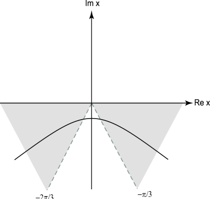
Figure 1: Stokes’ wedges in which the eigenfunctions $\psi(x)$ for the $-x^{4}$ eigenvalue problem (4) are required to vanish as $|x|\to\infty$. These wedges border on, but do not include the real axis. A possible path along which one can solve the eigenvalue differential equation is shown. This path must asymptote inside the Stokes’ wedges.

Step 1: Map the integration path onto the real axis by the change of variable

$$x=-2i\sqrt{1+it},\quad t\in(-\infty,\infty).$$ (5)

As $t$ runs along the real axis from $-\infty$ to $+\infty$, $x$ runs along the complex contour that asymptotes in the Stokes’ wedges shown in Fig. 1. Under the change of independent variable in (5), the derivatives transform as follows:

$$\,\,\,\textstyle{\frac{\rm d}{{\rm d}x}} = \sqrt{1+it}\,\textstyle{\frac{\rm d}{{\rm d}t}},$$ (6)

$$\left(\textstyle{\frac{\rm d}{{\rm d}x}}\right)^{2} = (1+it)\left(\textstyle{\frac{\rm d}{{\rm d}t}}\right)^{2}+\textstyle{\frac{1}{2}}i\textstyle{\frac{\rm d}{{\rm d}t}}.$$ (7)

Thus, with the substitution $\psi(x)=\phi(t)$, (4) becomes

$$-\textstyle{\frac{\hbar^{2}}{2m}}\left[(1+it)\phi^{\prime\prime}(t)+\textstyle{\frac{1}{2}}i\phi^{\prime}(t)\right]-16\gamma(1+it)^{2}\phi(t)=E\phi(t).$$ (8)

Step 2: Take the Fourier transform of (8). The Fourier transform of $\phi(t)$ is

$$f(p)=\int dt\,e^{ipt/\hbar}\phi(t),$$ (9)

so the Fourier transform of (8) is achieved by making the replacements

$$it\to\hbar\textstyle{\frac{\rm d}{{\rm d}p}}\quad{\rm and}\quad\textstyle{\frac{\rm d}{{\rm d}t}}\to-\frac{ip}{\hbar},$$ (10)

and we obtain

$$-16\gamma\hbar^{2}f^{\prime\prime}(p)+\hbar\left(\textstyle{\frac{p^{2}}{2m}}-32\gamma\right)f^{\prime}(p)+\left(\textstyle{\frac{p^{2}}{2m}}+\textstyle{\frac{3\hbar p}{4m}}-16\gamma\right)f(p)$$

$$\quad=Ef(p).$$ (11)

Step 3: Introduce the new dependent variable $g(p)$ by

$$f(p)=Q(p)g(p)$$ (12)

and choose $Q(p)$ to remove the one-derivative term and thereby change (11) to Schrödinger form. The condition on $Q(p)$ that eliminates terms containing $g^{\prime}(p)$ is

$$\textstyle{\frac{Q^{\prime}(p)}{Q(p)}}=\textstyle{\frac{p^{2}}{64m\gamma\hbar}}-\textstyle{\frac{1}{\hbar}}.$$ (13)

Differentiating (13), we get

$$\textstyle{\frac{Q^{\prime\prime}(p)}{Q(p)}}=\textstyle{\frac{p}{32m\gamma\hbar}}+\left(\textstyle{\frac{p^{2}}{64m\gamma\hbar}}-\textstyle{\frac{1}{\hbar}}\right)^{2}$$ (14)

and substituting (12 – 14) into (11), we obtain the Schrödinger equation

$$-16\gamma\hbar^{2}g^{\prime\prime}(p)+\left(\textstyle{\frac{p^{4}}{256m^{2}\gamma}}+\textstyle{\frac{\hbar p}{4m}}\right)g(p)=Eg(p).$$ (15)

Step 4: Finally, rescale the independent variable $p$:

$$p\to\sqrt{32m\gamma}\,p.$$ (16)

This rescaling makes (15) resemble the original Schrödinger equation in (4):

$$-\textstyle{\frac{\hbar^{2}}{2m}}g^{\prime\prime}(p)+\left(4\gamma p^{4}+\hbar\sqrt{\textstyle{\frac{2\gamma}{m}}}\,p\right)g(p)=Eg(p).$$ (17)

The Schrödinger equation (17) is associated with the Hamiltonian in (3). Since the differential equation (17) is real and the boundary conditions on the eigenfunctions $g(p)$ are imposed on the real axis, it follows that the eigenvalues are real. This constitutes a rigorous proof that the non-Hermitian Hamiltonian $\hat{H}_{2}$ in (2) has a real spectrum.

The term in (3) that is proportional to $\hbar$ is a quantum anomaly that arises as a remnant of the complex boundary conditions on the eigenfunctions associated with (4). (These boundary conditions are illustrated in Fig. 1.) In the classical limit $\hbar\to 0$, we obtain the classical Hamiltonian

$$K_{2,\,{\rm classical}}=\textstyle{\frac{1}{2m}}x^{2}+4\gamma p^{4}.$$ (18)

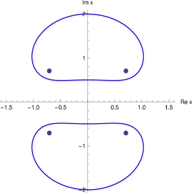
Figure 2: Classical ${\cal P}{\cal T}$-symmetric trajectories in the complex-$x$ plane for the Hamiltonian $H_{2,\,{\rm classical}}$ with $m=1/2$ and $\gamma=1$. For these trajectories the energy $E=1$ and the trajectories start at $2i$ and $-2i$. The period of the motion is $T=1.854\,074\,68\ldots\,~{}$.

It is an interesting but previously unnoticed fact that at the classical level the two Hamiltonians (2) and (18) are equivalent. To demonstrate this equivalence we show that the classical trajectories determined by these Hamiltonians in complex-coordinate space have identical periods. We plot in Fig. 2 two classical orbits of $H_{2,\,{\rm classical}}$ for $m=1/2$, $\gamma=1$, and energy $E=1$. Note that there are four turning points, which are located at $x=e^{i\pi/4}$, $x=e^{3i\pi/4}$, $x=e^{5i\pi/4}$, and $x=e^{7i\pi/4}$. A trajectory starting at $x=2i$ gives a closed orbit in the upper-half plane, and a trajectory starting at $x=-2i$ gives a closed orbit in the lower-half plane. Both orbits have the same period $T$, where

$$T=\frac{\sqrt{2\pi}\Gamma(1/4)}{4\Gamma(3/4)}=1.854\,074\,68\ldots\,.$$ (19)

We calculate $T$ by solving Hamilton’s equations ${\dot{x}}=\frac{\partial H}{\partial p}=2p$ and ${\dot{p}}=-\frac{\partial H}{\partial x}=4x^{3}$. Eliminating $p$, we express the period $T$ as the contour integral

$$T=\oint\frac{dx}{2\sqrt{1+x^{4}}}.$$ (20)

We then use Cauchy’s theorem to distort the contour to one that goes along a ray from the origin to a turning point, encircles the turning point, and follows the ray back to the origin. The contour then continues along another ray out to the other turning point, encircles this turning point, and follows that ray back to the origin. The resulting integral becomes a standard representation for a Beta function.

In Fig. 3 we plot the classical orbit for a particle of energy $E=1$ described by the Hamiltonian $K_{2,\,{\rm classical}}$ in (18). Note that there are now two and not four turning points located at $x=\pm 1$. The figure shows a closed periodic classical orbit that begins at $x=2i$. The period $T$ of this orbit is exactly that given in (19).

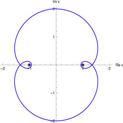
Figure 3: Classical ${\cal P}{\cal T}$-symmetric trajectories in the complex-$x$ plane for the $K_{2,\,{\rm classical}}$ Hamiltonian in (18). The period of this orbit is identical to the periods of the orbits shown in Fig. 2.

Figure 3 exhibits a remarkable new topological feature that is not found in the complex classical trajectories of Hamiltonians of the form $p^{2}+V(x)$, namely, that the classical orbit makes a $270^{\circ}$ loop around the turning points. There have been many studies of complex classical systems [2, 26, 27, 28, 29, 30, 31] and in previous numerical studies of complex trajectories the Hamiltonians that were examined were quadratic in the momentum $p$. When the momentum term in the Hamiltonian is quadratic, the trajectory always makes a $180^{\circ}$ U-turn about the turning points. In contrast, with Hamiltonians of the form $p^{3}+V(x)$, the classical trajectory makes a $240^{\circ}$ turn and for Hamiltonians of the form $p^{4}+V(x)$, the classical trajectory makes a $270^{\circ}$ turn about the turning points. These behaviors are illustrated in Fig. 4.

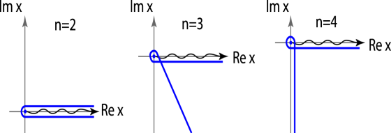
Figure 4: Behavior of a classical trajectory as it approaches a turning point of a Hamiltonian of the form $p^{n}+V(x)$ for $n=2$, $n=3$, and $n=4$. When $n=2$ the trajectory executes a $180^{\circ}$ U-turn, when $n=3$ the trajectory makes a $240^{\circ}$ turn, and when $n=4$ the trajectory makes a $270^{\circ}$ turn. The wiggly lines indicate that the turning point is a branch point of an $n$-sheeted Riemann surface. Turning points of the $n=3$ type are shown in Figs. 6 and 12 and turning points of the $n=4$ type are shown in Figs. 3 and 8.

To understand the angular rotation of a classical trajectory about a turning point, let us consider a Hamiltonian of the form $H=p^{n}+V(x)$. From the first of Hamilton’s equations, ${\dot{x}}=\frac{\partial H}{\partial p}=np^{n-1}$, we can eliminate $p$ from the Hamiltonian and we find that a particle of energy $E$ obeys the equation ${\dot{x}}=n[E-V(x)]^{(n-1)/n}$. We can now see that the turning point is also a branch point of an $n$-sheeted Riemann surface. Note that as $n\to\infty$, a classical trajectory that approaches a turning point will make a full $360^{\circ}$ turn and continue going in the same direction! (We encounter many examples of such higher-order turning points throughout this paper. However, we emphasize that, in general, the properties of higher-order classical turning points are not easy to predict analytically, and require the kind of sophisticated analysis used in catastrophe theory.)

The main objective of this paper is to show how to construct isospectral pairs of Hamiltonians, one of which is associated with a complex eigenvalue problem while the other is associated with a real eigenvalue problem. There have been many attempts to find isospectral pairs of Hamiltonians of the form $\hat{p}^{2}+V(\hat{x})$ by using the four-step differential-equation procedure outlined above. However, all such attempts have proved fruitless. In this paper we consider a wider class of Hamiltonians in which $\hat{p}^{2}$ is replaced by $\hat{p}^{n}$, and we suggest by means of illustrative examples (rather than by presenting a proof) that for each integer value of $n$ it is now possible to construct such an isospectral pair of ${\cal P}{\cal T}$-symmetric Hamiltonians. (To construct a proof, one would have to follow the procedure detailed in the illustrative examples in Secs. 3 and 4.) The eigenfunctions for the first member of the pair ${\hat{H}}_{n}$ satisfy boundary conditions in Stokes’ wedges in the complex plane. However, the eigenfunctions for the second member of the pair ${\hat{K}}_{n}$ satisfy a real differential equation with homogeneous boundary conditions given on the real axis. Therefore, our construction constitutes a rigorous proof that entire eigenspectrum of the complex Hamiltonian ${\hat{H}}_{n}$ is real.

The Hamiltonian $\hat{K}_{n}$ that is spectrally equivalent to $\hat{H}_{n}$ has quantum anomaly terms containing powers of $\hbar$ up to $n-1$. If we discard these anomaly terms, we obtain a pair of classical Hamiltonians that are equivalent in the following sense: For each closed periodic classical trajectory of the first Hamiltonian, it appears that there exists a closed trajectory of the second Hamiltonian that has exactly the same period.

This paper is organized as follows: In Sec. 2 we present some general introductory calculations. Then, in Secs. 3 and 4 we treat the cases $n=3$ and $n=4$. Finally, in Sec. 5 we make some concluding remarks.

2 General treatment

In order to carry out Step 1 on $\hat{H}_{n}$ in (3) we must generalize the mapping in (5):

$$x=-\frac{i}{\alpha}(1+it)^{\alpha},\quad t\in(-\infty,\infty),$$ (21)

where $\alpha=1/n$. Note that this change of variable reduces to (5) when $n=2$ ($\alpha=\textstyle{\frac{1}{2}}$). Now, as $t$ runs from $-\infty$ to $+\infty$ along the real axis, $x$ runs along a complex contour that is appropriate for the Hamiltonian $\hat{H}_{n}$.

The transformations from $x$ derivatives to $t$ derivatives can then be written as

$$\,\,\,\textstyle{\frac{\rm d}{{\rm d}x}} = (1+it)^{1-\alpha}\textstyle{\frac{\rm d}{{\rm d}t}},$$ (22)

$$\left(\textstyle{\frac{\rm d}{{\rm d}x}}\right)^{2} = (1+it)^{2-2\alpha}\left(\textstyle{\frac{\rm d}{{\rm d}t}}\right)^{2}+i(1-\alpha)(1+it)^{1-2\alpha}\textstyle{\frac{\rm d}{{\rm d}t}},$$ (23)

$$\left(\textstyle{\frac{\rm d}{{\rm d}x}}\right)^{3} = (1+it)^{3-3\alpha}\left(\textstyle{\frac{\rm d}{{\rm d}t}}\right)^{3}+3i(1-\alpha)(1+it)^{2-3\alpha}\left(\textstyle{\frac{\rm d}{{\rm d}t}}\right)^{2}$$ (24)

$$\qquad-(1-\alpha)(1-2\alpha)(1+it)^{1-3\alpha}\textstyle{\frac{\rm d}{{\rm d}t}},$$

$$\left(\textstyle{\frac{\rm d}{{\rm d}x}}\right)^{4} = (1+it)^{4-4\alpha}\left(\textstyle{\frac{\rm d}{{\rm d}t}}\right)^{4}+6i(1-\alpha)(1+it)^{3-4\alpha}\left(\textstyle{\frac{\rm d}{{\rm d}t}}\right)^{3}$$ (25)

$$\qquad-(1-\alpha)(7-11\alpha)(1+it)^{2-4\alpha}\left(\textstyle{\frac{\rm d}{{\rm d}t}}\right)^{2}$$

$$\qquad-i(1-\alpha)(1-2\alpha)(1-3\alpha)(1+it)^{1-4\alpha}\textstyle{\frac{\rm d}{{\rm d}t}}.$$

This set of equations generalizes (6) and (7); (22) and (23) reduce to (6) and (7) when $\alpha=\textstyle{\frac{1}{2}}$. In the next two sections we show how use these results to transform a general class of Hamiltonians of the form (1). Note that the Hamiltonian in (2) corresponds to $n=2$. We begin with the simplest generalization, namely, $n=3$.

3 Case $n=3$

In this section we consider the Hamiltonian (1) for the case $n=3$:

$$\hat{H}_{3}=\eta\hat{p}^{3}-i\gamma\hat{x}^{9}.$$ (26)

The corresponding differential-equation eigenvalue problem $\hat{H}_{3}\psi=E\psi$ is

$$i\hbar^{3}\eta\left(\textstyle{\frac{\rm d}{{\rm d}x}}\right)^{3}\psi(x)-i\gamma x^{9}\psi(x)=E\psi(x).$$ (27)

To solve this boundary-value problem the integration path must lie in Stokes’ wedges. For the above equation these wedges do not include the real axis. The wedges are determined by the asymptotic solutions to (27), which for large $|x|$ have the form $\exp(c\omega x^{4})$, where $c=\frac{1}{4\hbar}(\gamma/\eta)^{1/3}$ is a positive constant and $\omega$ is a cube root of unity: $\omega^{3}=1$. From this asymptotic behavior we see that each of the Stokes’ wedges has angular opening $\pi/4$. We impose boundary conditions in the wedges $-\pi/8>{\rm arg}\,x>-3\pi/8$ and $-5\pi/8>{\rm arg}\,x>-7\pi/8$. (These wedges are the shaded regions in the lower-half plane shown in Fig. 5.) Requiring that $\psi(x)$ vanish as $|x|\to\infty$ with ${\rm arg}\,x$ in the above two wedges eliminates two of the three possible solutions to (27) and keeps only the solution whose asymptotic behavior is given by $\exp(cx^{4})$.

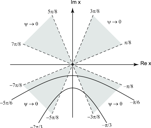
Figure 5: Stokes’ wedges for the solutions to the differential equation (27). The boundary conditions on the solution to this eigenvalue problem require that $\psi(x)\to 0$ as $|x|\to\infty$ with ${\rm arg}\,x$ inside the two shaded wedges in the lower-half plane. Two integration contours inside these wedges are shown, one of which runs from an angle of $-5\pi/6$ to an angle of $-\pi/6$ and the other from $-2\pi/3$ to $-\pi/3$. When we set $\alpha=\frac{1}{3}$ in (21) and allow $t$ to run from $-\infty$ to $\infty$, the variable $x$ follows the latter curve in the complex-$x$ plane.

We now follow Step 1 of the procedure explained in Sec. 1 and make the change of variable in (21) with $\alpha=\frac{1}{3}$. From (24) we then obtain the differential equation

$$i\hbar^{3}\eta\left[(1+it)^{2}\left(\textstyle{\frac{\rm d}{{\rm d}t}}\right)^{3}+2i(1+it)\left(\textstyle{\frac{\rm d}{{\rm d}t}}\right)^{2}-\textstyle{\frac{2}{9}}\textstyle{\frac{\rm d}{{\rm d}t}}\right]\phi(t)$$

$$\qquad-3^{9}\gamma(1+it)^{3}\phi(t)=E\phi(t).$$ (28)

This differential equation is to be solved on the real axis in the $t$ variable and the solution satisfies homogeneous boundary conditions on the real axis. Note that as $t$ runs from $-\infty$ to $\infty$, the variable $x$ runs from an angle of $-2\pi/3$ to an angle of $-\pi/3$ in the complex-$x$ plane. This integration in the complex-$x$ plane is shown in Fig. 5.

Following Step 2, we perform the Fourier transform in (9) and use (10) to obtain

$$\eta\left[-\left(1+\hbar\textstyle{\frac{\rm d}{{\rm d}p}}\right)^{2}p^{3}+2\hbar\left(1+\hbar\textstyle{\frac{\rm d}{{\rm d}p}}\right)p^{2}-\textstyle{\frac{2}{9}}\hbar^{2}p\right]f(p)$$

$$\qquad-3^{9}\gamma\left(1+\hbar\textstyle{\frac{\rm d}{{\rm d}p}}\right)^{3}f(p)=Ef(p).$$ (29)

We then simplify (29) by transforming it to a new differential equation that does not have a second-derivative term. To do so we let $f(p)=Q(p)g(p)$, as in Step 3 of Sec. 1. The condition on $Q(p)$ that eliminates the second-derivative term is

$$\textstyle{\frac{Q^{\prime}(p)}{Q(p)}}=-\textstyle{\frac{1}{\hbar}}-\textstyle{\frac{\eta p^{3}}{3^{10}\gamma\hbar}},$$ (30)

and upon differentiation we get

$$\textstyle{\frac{Q^{\prime\prime}(p)}{Q(p)}} = \textstyle{\frac{1}{\hbar^{2}}}-\textstyle{\frac{\eta p^{2}}{3^{9}\gamma\hbar}}+\textstyle{\frac{\eta^{2}p^{6}}{3^{20}\gamma^{2}\hbar^{2}}}+\textstyle{\frac{2\eta p^{3}}{3^{10}\gamma\hbar^{2}}},$$

$$\textstyle{\frac{Q^{\prime\prime\prime}(p)}{Q(p)}} = -\textstyle{\frac{1}{\hbar^{3}}}-\textstyle{\frac{2\eta p}{3^{9}\gamma\hbar}}+\textstyle{\frac{\eta^{2}p^{5}}{3^{18}\gamma^{2}\hbar^{2}}}+\textstyle{\frac{\eta p^{2}}{3^{8}\gamma\hbar^{2}}}-\textstyle{\frac{\eta^{2}p^{6}}{3^{19}\gamma^{2}\hbar^{3}}}-\textstyle{\frac{\eta p^{3}}{3^{9}\gamma\hbar^{3}}}-\textstyle{\frac{\eta^{3}p^{9}}{3^{30}\gamma^{3}\hbar^{3}}}.$$ (31)

The resulting equation for $g(p)$ is

$$-3^{9}\gamma\hbar^{3}g^{\prime\prime\prime}(p)+\left(\textstyle{\frac{\eta^{2}\hbar p^{6}}{3^{10}\gamma}}-\eta\hbar^{2}p^{2}\right)g^{\prime}(p)$$

$$\qquad+\left(\textstyle{\frac{4\eta^{2}\hbar p^{5}}{3^{10}\gamma}}-\textstyle{\frac{2\eta\hbar^{2}p}{9}}-\textstyle{\frac{2\eta^{3}p^{9}}{3^{21}\gamma^{2}}}\right)g(p)=Eg(p).$$ (32)

This completes Step 3.

Finally, we perform the scaling

$$p\to\textstyle{\frac{27\gamma^{1/3}}{\eta^{1/3}}}p$$ (33)

and obtain

$$-\eta\hbar^{3}g^{\prime\prime\prime}(p)+\left(-27\eta^{2/3}\gamma^{1/3}\hbar^{2}p^{2}+243\eta^{1/3}\gamma^{2/3}\hbar p^{6}\right)g^{\prime}(p)$$

$$\qquad+\left(972\eta^{1/3}\gamma^{2/3}\hbar p^{5}-6\eta^{2/3}\gamma^{1/3}\hbar^{2}p+1458\gamma p^{9}\right)g(p)=Eg(p).$$ (34)

This completes Step 4 and from this result we make the ansatz $\textstyle{\frac{\rm d}{{\rm d}p}}\to\frac{i}{\hbar}\hat{x}$ to identify the Hamiltonian that is equivalent to that in (26):

$$\hat{K}_{3}=i\eta\hat{x}^{3}+i\left(-27\eta^{2/3}\gamma^{1/3}\hbar\hat{p}^{2}+243\eta^{1/3}\gamma^{2/3}\hat{p}^{6}\right)\hat{x}$$

$$\qquad+\left(972\eta^{1/3}\gamma^{2/3}\hbar\hat{p}^{5}-6\eta^{2/3}\gamma^{1/3}\hbar^{2}\hat{p}+1458\gamma\hat{p}^{9}\right).$$ (35)

Observe that there is an $\hbar^{2}$ anomaly term as well as two $\hbar$ anomaly terms. Therefore, in the classical limit $\hbar\to 0$, $\hat{K}_{3}$ in (35) becomes

$$K_{3,\,{\rm classical}}=i\eta x^{3}+243i\eta^{1/3}\gamma^{2/3}p^{6}x+1458\gamma p^{9}.$$ (36)

We now argue that the two classical Hamiltonians, $H_{3,\,{\rm classical}}$ and $K_{3,\,{\rm classical}}$, are equivalent by computing numerically the classical trajectories for each Hamiltonian and verifying that trajectories having the same energy have the same periods. In Fig. 6 we plot a classical trajectory for $H_{3,\,{\rm classical}}$ with $\eta=1$ and $\gamma=1$ for a particle of energy $E=1$ starting at $x=0.5\,i$.

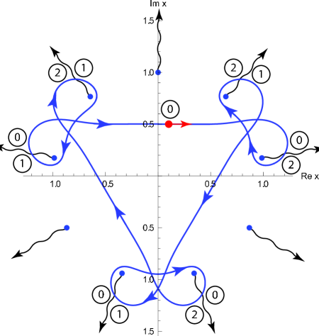
Figure 6: A classical ${\cal P}{\cal T}$-symmetric periodic trajectory in the complex-$x$ plane for the Hamiltonian $H_{3,\,{\rm classical}}=p^{3}-ix^{9}$ for a particle of energy $E=1$. The trajectory begins at $x=0.5\,i$ and proceeds to wind around six of the nine turning points. It never crosses itself because each of the turning points is a cube-root branch point, and thus the trajectory visits the three sheets of the Riemann surface, which are numbered 0, 1, and 2. The period of the motion is $T=3.377\,981\,999\,015\ldots$ .

The trajectory in Fig. 6 has an elaborate structure. It winds around six of the nine turning points in the negative (clockwise) direction. Because each of the nine turning points is also a branch point of cubic type, with each wind the direction of the path changes by $240^{\circ}$, as shown in Fig. 4. Thus, after the path leaves its starting point at $x=0.5\,i$, it winds in the negative direction and crosses from sheet zero to sheet two of the Riemann surface (which is equivalent to sheet $-1$). The number of the sheet is indicated in a circle on Fig. 6. The path then heads upward and to the left, but it does not cross itself because it is on the second sheet and no longer on the zeroth sheet. The path then proceeds to visit each sheet of the Riemann surface twice before returning to its starting point at $x=0.5\,i$ on the zeroth sheet.

We can calculate the period of this orbit exactly by distorting the path shown in Fig. 6 into a path that begins at the origin, travels outward to a turning point along a ray, encircles the turning point, and then returns to the origin, and then repeats this trip five more times. However, in evaluating the complex line integrals we must be careful to remember that the phase of the integrand changes as the path encircles the turning point. Upon adding together the contributions from all six turning points we obtain the exact result $T=2[\cos(\pi/18)+\cos(7\pi/18)]\Gamma(10/9)\Gamma(1/3)/\Gamma(4/9)=3.377\,981\,999\,015\ldots~{}.$

In Fig. 7 we plot the classical trajectory of a particle of energy $E=1$ governed by the Hamiltonian $K_{3,\,{\rm classical}}$ with $\eta=1$ and $\gamma=1$. This trajectory begins at $x=0$. The time for the particle to follow the path shown in this figure is $T=1.125\,994\ldots$, which is precisely $1/3$ of the period of the closed orbit shown in Fig. 6. We emphasize that the trajectory of this orbit is not yet closed. Figure 7 shows that the particle must trace this path three times before the orbit closes, and the time required to do this is exactly the period of the orbit shown in Fig. 6.

One might think (wrongly!) that there should be a total of six rather than three turning points on Fig. 7. We determine the positions of the turning points from the first of Hamilton’s equations

$$\dot{x}=\frac{\partial}{\partial p}K_{3,\,{\rm classical}}=3^{6}2ip^{5}x+3^{8}2p^{8}.$$ (37)

The turning points are the points where $\dot{x}=0$, and this seems to occur when $p=0$ and when $ix+9p^{3}=0$. However, if we then substitute each of these conditions into the equation $K_{3,\,{\rm classical}}=1$, we find that only the first of these conditions is consistent, so we learn that there are three turning points situated at the three roots of $-i$. The second condition is inconsistent.

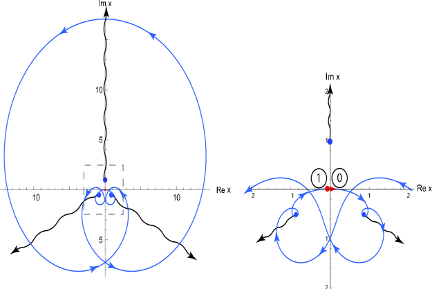
Figure 7: A classical ${\cal P}{\cal T}$-symmetric trajectory in the complex-$x$ plane for the Hamiltonian $K_{3,\,{\rm classical}}$ in (35) with $\eta=1$ and $\gamma=1$. The trajectory shown is that of a particle of energy $E=1$ beginning at $x=-i$. The trajectory follows an elaborate and complicated path as it winds around the three turning points, which are indicated by dots. The inset shows a blown-up version of the trajectory near the origin. Note that the trajectory never crosses itself because each of the turning points is also a cube-root branch point, and thus the trajectory lies in a three-sheeted Riemann surface. The period of the orbit is $T=1.125\,994\ldots$, which is exactly $1/3$ of the period of the closed orbit shown in Fig. 6. It is crucial to observe that the trajectory shown is not closed; the inset indicates that if the trajectory is on sheet 0 just to the right of the origin, it returns to this point on sheet 1. Thus, it must trace this path two more times before it closes. When it finally closes, the period of its orbit agrees exactly with that of the trajectory shown in Fig. 6.

4 Case $n=4$

In this section we consider the Hamiltonian

$$\hat{H}_{4}=\eta\hat{p}^{4}-\gamma\hat{x}^{16}.$$ (38)

The substitution $\hat{p}=-i\hbar\textstyle{\frac{\rm d}{{\rm d}x}}$ converts the formal eigenvalue problem $\hat{H}_{4}\psi=E\psi$ into the differential-equation eigenvalue problem

$$\eta\hbar^{4}\left(\textstyle{\frac{\rm d}{{\rm d}x}}\right)^{4}\psi(x)-\gamma x^{16}\psi(x)=E\psi(x).$$ (39)

The asymptotic behavior of the eigenfunctions $\psi(x)$ has the form $\exp(icx^{5}/5)$, where $c=\frac{1}{5\hbar}(\gamma/\eta)^{1/4}$ is a positive constant. Thus, the eigenfunctions vanish exponentially fast in a pair of ${\cal P}{\cal T}$-symmetric wedges in the lower-half complex-$x$ plane centered about $-3\pi/10$ and $-7\pi/10$.

Step 1: We map this differential-equation eigenvalue problem onto the real axis by taking $\alpha=\frac{1}{4}$ in (21) so that $x=(1-it)^{1/4}$. The mapped eigenvalue problem is

$$\eta\hbar^{4}\left[(1+it)^{3}\left(\textstyle{\frac{\rm d}{{\rm d}t}}\right)^{4}+\textstyle{\frac{9}{2}}i(1+it)^{2}\left(\textstyle{\frac{\rm d}{{\rm d}t}}\right)^{3}-\textstyle{\frac{51}{16}}(1+it)\left(\textstyle{\frac{\rm d}{{\rm d}t}}\right)^{2}-\textstyle{\frac{3}{32}}i\textstyle{\frac{\rm d}{{\rm d}t}}\right]\phi(t)$$

$$\qquad-4^{16}\gamma(1+it)^{4}\phi(t)=E\phi(t).$$ (40)

Step 2: Taking the Fourier Transform of (40), we get

$$\eta\hbar^{4}\left[\left(1+\hbar\textstyle{\frac{\rm d}{{\rm d}p}}\right)^{3}\textstyle{\frac{p^{4}}{\hbar^{4}}}-\textstyle{\frac{9}{2}}\left(1+\hbar\textstyle{\frac{\rm d}{{\rm d}p}}\right)^{2}\textstyle{\frac{p^{3}}{\hbar^{3}}}+\textstyle{\frac{51}{16}}\left(1+\hbar\textstyle{\frac{\rm d}{{\rm d}p}}\right)\textstyle{\frac{p^{2}}{\hbar^{2}}}-\textstyle{\frac{3}{32}}\textstyle{\frac{p}{\hbar}}\right]f(p)$$

$$\qquad-4^{16}\gamma\left(1+\hbar\textstyle{\frac{\rm d}{{\rm d}p}}\right)^{4}f(p)=Ef(p).$$ (41)

Step 3: We transform the dependent variable using $f(p)=Q(p)g(p)$ and choose $Q(p)$ to eliminate the third-derivative term $g^{\prime\prime\prime}(p)$. The function $Q(p)$ that does this is

$$Q(p)=\exp\left(-\textstyle{\frac{p}{\hbar}}+\textstyle{\frac{\eta p^{5}}{4^{17}5\gamma\hbar}}\right).$$ (42)

The result in (42) simplifies (41) to

$$-4^{16}\hbar^{4}\gamma g^{\prime\prime\prime\prime}(p)+\textstyle{\frac{3p^{16}\eta^{4}}{4^{52}\gamma^{3}}}g(p)+\textstyle{\frac{\hbar\eta^{3}}{4^{35}\gamma^{2}}}\left[8p^{12}g^{\prime}(p)+54p^{11}g(p)\right]$$

$$\quad+\textstyle{\frac{\hbar^{2}\eta^{2}}{4^{19}\gamma}}\left[24p^{8}g^{\prime\prime}(p)+240p^{7}g^{\prime}(p)+483p^{6}g(p)\right]$$

$$\quad-\textstyle{\frac{\hbar^{3}\eta}{32}}\left[-48p^{3}g^{\prime\prime}(p)-6p^{2}g^{\prime}(p)+87pg(p)\right]=Eg(p).$$ (43)

Step 4: Next, we perform the scaling transformation

$$p\to\textstyle{\frac{4^{4}\gamma^{1/4}}{\eta^{1/4}}}p$$ (44)

and obtain the real eigenvalue problem

$$-\eta\hbar^{4}g^{\prime\prime\prime\prime}(p)+4^{12}3\gamma p^{16}g(p)+\hbar 4^{9}\gamma^{3/4}\eta^{1/4}\left[8p^{12}g^{\prime}(p)+54p^{11}g(p)\right]$$

$$\quad+\hbar^{2}4^{5}\sqrt{\gamma\eta}\left[24p^{8}g^{\prime\prime}(p)+240p^{7}g^{\prime}(p)+483p^{6}g(p)\right]$$

$$\quad-8\hbar^{3}\gamma^{1/4}\eta^{3/4}\left[-48p^{3}g^{\prime\prime}(p)-6p^{2}g^{\prime}(p)+87pg(p)\right]=Eg(p),$$ (45)

whose boundary conditions are posed on the real axis. Finally, we identify the Hamiltonian that gives rise to this eigenvalue problem by substituting $\textstyle{\frac{\rm d}{{\rm d}p}}\to\frac{i}{\hbar}\hat{x}$:

$$\hat{K}_{4} = -\eta\hat{x}^{4}+4^{12}3\gamma\hat{p}^{16}+4^{9}\gamma^{3/4}\eta^{1/4}\left(8i\hat{p}^{12}\hat{x}+54\hbar\hat{p}^{11}\right)$$ (46)

$$\quad+4^{5}\sqrt{\gamma\eta}\left(-24\hat{p}^{8}\hat{x}^{2}+240\hbar i\hat{p}^{7}\hat{x}+483\hbar^{2}\hat{p}^{6}\right)$$

$$\quad-8\gamma^{1/4}\eta^{3/4}\left(48\hbar\hat{p}^{3}\hat{x}^{2}-6i\hbar^{2}\hat{p}^{2}\hat{x}+87\hbar^{3}\hat{p}\right).$$

We have thus shown that the eigenvalues of $\hat{K}_{4}$ are real and are identical to the eigenvalues of $\hat{H}_{4}$.

Notice that $\hat{K}_{4}$ has first-, second-, and third-order anomaly terms. In the classical limit $\hbar\to 0$ we obtain

$$K_{4,\,{\rm classical}}=-2^{13}3\sqrt{\gamma\eta}\,p^{8}x^{2}-\eta x^{4}+2^{21}i\gamma^{3/4}\eta^{1/4}p^{12}x+2^{24}3\gamma p^{16}.$$ (47)

We will now demonstrate that the two classical Hamiltonians, $H_{4,\,{\rm classical}}$ and $K_{4,\,{\rm classical}}$, are equivalent by showing that the classical periods of the motion are identical.

Let us first examine the complex particle motion due to $H_{4,\,{\rm classical}}$ for the case $\eta=1$ and $\gamma=1$. In Fig. 8 we plot a closed orbit of a particle of energy $E=1$ that begins at $0.8i$. The orbit takes the approximate shape of a rectangle and makes $270^{\circ}$ turns at the four corners. The period of this orbit is $T=1.697\,723\,019\,533\ldots$ . We can calculate this period exactly by distorting it into rays that go from the origin out to each of the turning points and back to the origin, taking great care to keep track of the phase of the integrand. The exact formula for the period is $T=[\cos(3\pi/16)+\cos(5\pi/16)]\Gamma(1/4)\Gamma(17/16)/\Gamma(5/16)$.

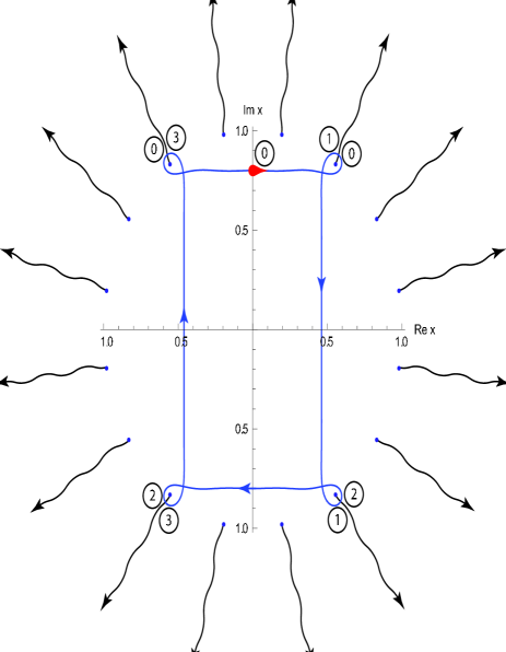
Figure 8: A classical ${\cal P}{\cal T}$-symmetric periodic trajectory in the complex-$x$ plane for the Hamiltonian $H_{4,\,{\rm classical}}=p^{4}-x^{16}$ for a particle of energy $E=1$. The trajectory begins at $x=0.8i$ and proceeds to wind around four of the 16 turning points. It never crosses itself because each of the turning points is a fourth-root branch point, and thus the trajectory visits the four sheets of the Riemann surface, which are numbered 0, 1, 2, and 3. The period of the motion is $T=1.697\,723\,019\,533\ldots$ .

Next, we examine the classical trajectories of $K_{4,\,{\rm classical}}$ for the case $\eta=1$ and $\gamma=1$. In Fig. 9 we plot the classical trajectory for a particle of $E=1$ that begins at $x=-i$. There are four turning points of fourth-root type. However, in this figure it is not possible to see the detailed structure of this trajectory near the origin. Therefore, in Fig. 10 we plot a blow-up of the square region in Fig. 9 near the origin.

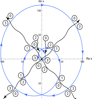
Figure 9: A classical trajectory in the complex-$x$ plane for the Hamiltonian $K_{4,\,{\rm classical}}$ in (47) with $\eta=1$ and $\gamma=1$. The trajectory represents a particle of energy $E=1$ that begins at $x=e^{-i\pi/4}$. The trajectory winds around the turning points in a complicated fashion (see nested insets in Figs. 10 and 11) but it never crosses itself because it is on a multisheeted Riemann surface with each of the turning points being a fourth-root branch point. The trajectory returns to its starting point in time $T=0.848\,86$, but it is not a closed trajectory; the trajectory begins on sheet 0 and returns on sheet two of the Riemann surface. To complete its periodic motion the trajectory must follow the same path one more time. The time needed to complete this double loop is exactly equal to the period of the orbit shown in Fig. 8.

In Fig. 10 we can now see the four turning points and a rather complicated trajectory. The regions surrounding the upper pair of turning points have a highly detailed structure, and thus the square region surrounding the upper-right turning point is blown up again in Fig. 11 (left side). The vicinity of the turning point contains additional structure, and this region must be blown up still more in Fig. 11 (right side).

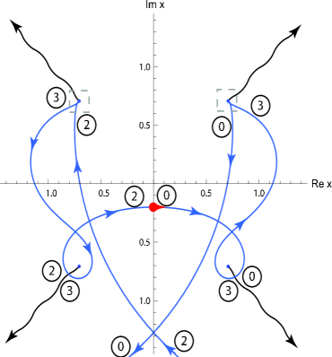
Figure 10: A blown-up view of the trajectory shown in Fig. 9 (see inset in Fig. 9). The four fourth-root turning points are visible in this figure. However, the trajectory has a complicated structure near the upper two turning points, and Fig. 11 shows a detail of the small region surrounding the upper-right turning point.

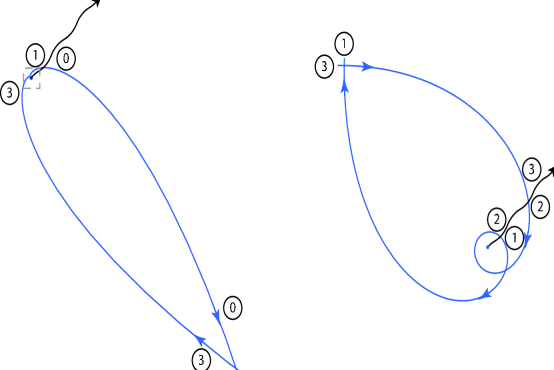
Figure 11: Left: A blown-up view of a portion of Fig. 10 (see inset in Fig. 10). Right: A blown-up view of the inset on the left side.

5 Summary

We have shown by using a number of examples that it is possible to construct an infinite tower of pairs of isospectral Hamiltonians $\hat{H}_{n}$ and $\hat{K}_{n}$, for which the first member of the pair is a complex ${\cal P}{\cal T}$-symmetric Hamiltonian. The differential-equation eigenvalue problem for the second Hamiltonian is entirely real, and therefore the eigenvalues of both Hamiltonians are real. The second member of the pair has quantum anomalies of order $\hbar^{n-1}$. We have also shown that at the classical level, where the anomaly terms in $\hat{K}_{n}$ are discarded, the Hamiltonians are equivalent by demonstrating that they have closed orbits of the same period.

Many unsolved problems remain. For example, we do not know if for every classical orbit of the Hamiltonians $H_{n,\,{\rm classical}}$ there is a corresponding classical orbit of the Hamiltonians $K_{n,\,{\rm classical}}$ of exactly the same period. Because complex coordinate space is a Riemann surface having an elaborate sheet structure, it is possible to find various classical orbits having many different periods. For example, for the classical Hamiltonian $H_{3,\,{\rm classical}}$ with $\eta=1$ and $\gamma=1$, we find that a particle of energy $E=1$ that starts at $x=1$ has a closed trajectory of period $T=6[\cos(\pi/18)+\cos(5\pi/18)]\Gamma(10/9)\Gamma(4/3)/\Gamma(4/9)=4.143\,708\,353\ldots$ . This orbit is shown in Fig. 12.

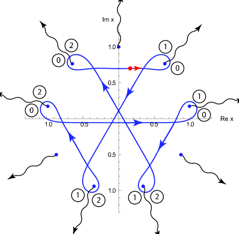
Figure 12: A classical ${\cal P}{\cal T}$-symmetric periodic trajectory in the complex-$x$ plane for the Hamiltonian $H_{3,\,{\rm classical}}=p^{3}-ix^{9}$ for a particle of energy $E=1$. The trajectory begins at $x=1$ and proceeds to wind around six of the nine turning points. It never crosses itself because each of the turning points is a cube-root branch point, and thus the trajectory visits the three sheets of a Riemann surface, which are numbered 0, 1, and 2. The period of the motion is $T=4.143\,708\,353\ldots$ .

We calculate the period of this orbit exactly by distorting the path shown in Fig. 12 into a path that begins at the origin, travels outward to a turning point along a ray, encircles the turning point, and then returns to the origin, and then repeats this trip five more times. In the complex line integrals the phase for each path advances as the path encircles the turning point. Upon adding together the contributions from all six turning points we obtain an analytic expression for the period of the motion. Although we are convinced that one exists, we have not yet been able to find a corresponding orbit of the Hamiltonian $K_{3,\,{\rm classical}}$.

CMB is supported by a grant from the U.S. Department of Energy.

References

[1] C. M. Bender and S. Boettcher, Phys. Rev. Lett., 80, 5243
(1998).
[2] C. M. Bender, S. Boettcher, and P. N. Meisinger,
J. Math. Phys. 40, 2201-2229 (1999).
[3] P. Dorey, C. Dunning, and R. Tateo, J. Phys. A: Math. Gen. 34, L391 (2001); ibid. 34, 5679 (2001).
[4] C. M. Bender, D. C. Brody, and H. F. Jones, Phys. Rev. Lett. 89, 270401 (2002); Am. J. Phys. 71, 1095 (2003).
[5] C. M. Bender, Contemp. Phys. 46, 277 (2005).
[6] C. M. Bender, Rep. Prog. Phys. 70, 947-1018 (2007).
[7] P. Dorey, C. Dunning, and R. Tateo, J. Phys. A: Math. Gen. 40, R205 (2007).
[8] A. A. Andrianov, Ann. Phys. (N.Y.) 140, 82 (1982).
[9] V. Buslaev and V. Grecchi, J. Phys. A 26, 5541 (1993).
[10] H. F. Jones and J. Mateo, Phys. Rev. D73, 085002 (2006).
[11] C. M. Bender, D. C. Brody, J.-H. Chen, H. F. Jones, K. A. Milton,
and M. C. Ogilvie, Phys. Rev. D 74, 025016 (2006).
[12] H. F. Jones, J. Mateo, R. J. Rivers, Phys. Rev. D 74,
125022 (2006).
[13] A. A. Andrianov, Phys. Rev. D 76, 025003 (2007).
[14] H. F. Jones and R. J. Rivers, Phys. Rev. D 75, 025023
(2007).
[15] F. Scholtz, H. Geyer, and F. Hahne, Ann. Phys. 213, 74
(1992).
[16] A. Mostafazadeh, J. Phys. A: Math. Gen. 36, 7081 (2003).
[17] H. F. Jones, J. Phys. A: Math. Gen. 38, 1741 (2005).
[18] A. Mostafazadeh, J. Phys. A: Math. Gen. 38, 6557 (2005);
Erratum ibid. 8185.
[19] C. M. Bender, S. F. Brandt, J.-H. Chen, and Q. Wang,
Phys. Rev. D 71, 025014 (2005).
[20] C. M. Bender and P. D. Mannheim, arXiv: hep-th/0706.0207.
[21] H. F. Jones, arXiv: hep-th/0711.4967.
[22] D. Krejcirik, H. Bila, and M. Znojil, J. Phys. A:
Math. Gen. 39, 10143 (2006).
[23] A. Mostafazadeh, J. Phys. A: Math. Gen. 39, 13495 (2006).
[24] D. P. Musumbu, H. B. Geyer, and W. D. Heiss, J. Phys. A:
Math. Theor. 40, F75 (2007).
[25] P. E. G. Assis and A. Fring, arXiv: 0708.2403.
[26] C. M. Bender, D. D. Holm, and D. W. Hook, J. Phys. A:
Math. Theor. 40, F81-F89 (2007).
[27] C. M. Bender, D. D. Holm, and D. W. Hook, J. Phys. A:
Math. Theor. 40, F793-F804 (2007).
[28] C. M. Bender, J.-H. Chen, D. W. Darg, and K. A. Milton,
J. Phys. A: Math. Gen. 39, 4219-4238 (2006).
[29] A. Fring, J. Phys. A: Math. Theor. 40, 4215 (2007).
[30] C. M. Bender and D. W. Darg, J. Math. Phys. 48, 042703
(2007).
[31] A. Nanayakkara, Czech. J. Phys. 54, 101 (2004) and
J. Phys. A: Math. Gen. 37, 4321 (2004).