Quantifying Homology Classes

Abstract.

We develop a method for measuring homology classes. This involves three problems. First, we define the size of a homology class, using ideas from relative homology. Second, we define an optimal basis of a homology group to be the basis whose elements’ size have the minimal sum. We provide a greedy algorithm to compute the optimal basis and measure classes in it. The algorithm runs in $O(\beta^{4}n^{3}\log^{2}n)$ time, where $n$ is the size of the simplicial complex and $\beta$ is the Betti number of the homology group. Third, we discuss different ways of localizing homology classes and prove some hardness results.

2008169-180Bordeaux 169

1. Introduction

The problem of computing the topological features of a space has recently drawn much attention from researchers in various fields, such as high-dimensional data analysis [3, 15], graphics [13, 5], networks [10] and computational biology [1, 8]. Topological features are often preferable to purely geometric features, as they are more qualitative and global, and tend to be more robust. If the goal is to characterize a space, therefore, features which incorporate topology seem to be good candidates.

Once we are able to compute topological features, a natural problem is to rank the features according to their importance. The significance of this problem can be justified from two perspectives. First, unavoidable errors are introduced in data acquisition, in the form of traditional signal noise, and finite sampling of continuous spaces. These errors may lead to the presence of many small topological features that are not “real”, but are simply artifacts of noise or of sampling [19]. Second, many problems are naturally hierarchical. This hierarchy – which is a kind of multiscale or multi-resolution decomposition – implies that we want to capture the large scale features first. See Figure 1 and 1 for examples.

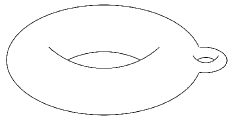
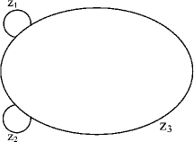
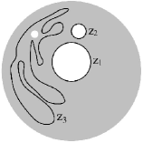
Figure 1. (a,b) A disk with three holes and a 2-handled torus are really more like an annulus and a 1-handled torus, respectively, because the large features are more important. (c) A topological space formed from three circles. (d) In a disk with three holes, cycles $z_{1}$ and $z_{2}$ are well-localized; $z_{3}$ is not.

The topological features we use are homology groups over $\mathbb{Z}_{2}$, due to their ease of computation. (Thus, throughout this paper, all the additions are mod 2 additions.) We would then like to quantify or measure homology classes, as well as collections of classes. Specifically, there are three problems we would like to solve:

1. Measuring the size of a homology class: We need a way to quantify the size of a given homology class, and this size measure should agree with intuition. For example, in Figure 1, the measure should be able to distinguish the one large class (of the 1-dimensional homology group) from the two smaller classes. Furthermore, the measure should be easy to compute, and applicable to homology groups of any dimension.

2. Choosing a basis for a homology group: We would like to choose a “good” set of homology classes to be the generators for the homology group (of a fixed dimension). Suppose that $\beta$ is the dimension of this group, and that we are using $\mathbb{Z}_{2}$ coefficients; then there are $2^{\beta}-1$ nontrivial homology classes in total. For a basis, we need to choose a subset of $\beta$ of these classes, subject to the constraint that these $\beta$ generate the group. The criterion of goodness for a basis is based on an overall size measure for the basis, which relies in turn on the size measure for its constituent classes. For instance, in Figure 1, we must choose three from the seven nontrivial $1$-dimensional homology classes: $\{[z_{1}],[z_{2}],[z_{3}],[z_{1}]+[z_{2}],[z_{1}]+[z_{3}],[z_{2}]+[z_{3}],[z_{1}]+[z_{2}]+[z_{3}]\}$. In this case, the intuitive choice is $\{[z_{1}],[z_{2}],[z_{3}]\}$, as this choice reflects the fact that there is really only one large cycle.

3. Localization: We need the smallest cycle to represent a homology class, given a natural criterion of the size of a cycle. The criterion should be deliberately chosen so that the corresponding smallest cycle is both mathematically natural and intuitive. Such a cycle is a “well-localized” representative of its class. For example, in Figure 1, the cycles $z_{1}$ and $z_{2}$ are well-localized representatives of their respective homology classes; whereas $z_{3}$ is not.

Furthermore, we make two additional requirements on the solution of aforementioned problems. First, the solution ought to be computable for topological spaces of arbitrary dimension. Second the solution should not require that the topological space be embedded, for example in a Euclidean space; and if the space is embedded, the solution should not make use of the embedding. These requirements are natural from the theoretical point of view, but may also be justified based on real applications. In machine learning, it is often assumed that the data lives on a manifold whose dimension is much smaller than the dimension of the embedding space. In the study of shape, it is common to enrich the shape with other quantities, such as curvature, or color and other physical quantities. This leads to high dimensional manifolds (e.g, 5-7 dimensions) embedded in high dimensional ambient spaces [4].

Although there are existing techniques for approaching the problems we have laid out, to our knowledge, there are no definitions and algorithms satisfying the two requirements. Ordinary persistence [12, 20, 6] provides a measure of size, but only for those inessential classes, i.e. classes which ultimately die. More recent work [7] attempts to remedy this situation, but not in an intuitive way. Zomorodian and Carlsson [21] use advanced algebraic topological machinery to solve the basis computation and localization problems. However, both the quality of the result and the complexity depend strongly on the choice of the given cover; there is, as yet, no suggestion of a canonical cover. Other works like [14, 19, 11] are restricted to low dimension.

Contributions.

In this paper, we solve these problems. Our contributions include:

• Definitions of the size of homology classes and the optimal homology basis.

• A provably correct greedy algorithm to compute the optimal homology basis and measure its classes. This algorithm uses the persistent homology.

• An improvement of the straightforward algorithm using finite field linear algebra.

• Hardness results concerning the localization of homology classes.

2. Defining the Problem

In this section, we provide a technique for ranking homology classes according to their importance. Specifically, we solve the first two problems mentioned in Section 1 by formally defining (1) a meaningful size measure for homology classes that is computable in arbitrary dimension; and (2) an optimal homology basis which distinguishes large classes from small ones effectively.

Since we restrict our work to homology groups over $\mathbb{Z}_{2}$, when we talk about a $d$-dimensional chain, $c$, we refer to either a collection of $d$-simplices, or a $n_{d}$-dimensional vector over $\mathbb{Z}_{2}$ field, whose non-zero entries corresponds to the included $d$-simplices. $n_{d}$ is the number of $d$-dimensional simplces in the given complex, $K$. The relevant background in homology and relative homology can be found in [16].

The Discrete Geodesic Distance

In order to measure the size of homology classes, we need a notion of distance. As we will deal with a simplicial complex $K$, it is most natural to introduce a discrete metric, and corresponding distance functions. We define the discrete geodesic distance from a vertex $p\in\operatorname*{vert}(K)$, $f_{p}:\operatorname*{vert}(K)\to\mathbb{Z}$, as follows. For any vertex $q\in\operatorname*{vert}(K)$, $f_{p}(q)=\operatorname*{dist}(p,q)$ is the length of the shortest path connecting $p$ and $q$, in the $1$-skeleton of $K$; it is assumed that each edge length is one, though this can easily be changed. We may then extend this distance function from vertices to higher dimensional simplices naturally. For any simplex $\sigma\in K$, $f_{p}(\sigma)$ is the maximal function value of the vertices of $\sigma$, $f_{p}(\sigma)=\max_{q\in\operatorname*{vert}(\sigma)}f_{p}(q)$. Finally, we define a discrete geodesic ball $B_{p}^{r}$, $p\in\operatorname*{vert}(K)$, $r\geq 0$, as the subset of $K$, $B_{p}^{r}=\{\sigma\in K\mid f_{p}(\sigma)\leq r\}$. It is straightforward to show that these subsets are in fact subcomplexes, namely, subsets that are still simplicial complexes.

2.1. Measuring the Size of a Homology Class

We start this section by introducing notions from relative homology. Given a simplicial complex $K$ and a subcomplex $L\subseteq K$, we may wish to study the structure of $K$ by ignoring all the chains in $L$. We study the group of relative chain as a quotient group, $\mathsf{C}_{d}(K,L)=\mathsf{C}_{d}(K)/\mathsf{C}_{d}(L)$, whose elements are relative chains. Analogous to the way we define the group of cycles $\mathsf{Z}_{d}(K)$, the group of boundaries $\mathsf{B}_{d}(K)$ and the homology group $\mathsf{H}_{d}(K)$ in $\mathsf{C}_{d}(K)$, we define the group of relative cycles, the group of relative boundaries and the relative homology group in $\mathsf{C}_{d}(K,L)$, denoted as $\mathsf{Z}_{d}(K,L)$, $\mathsf{B}_{d}(K,L)$ and $\mathsf{H}_{d}(K,L)$, respectively. We denote $\phi_{L}:\mathsf{C}_{d}(K)\to\mathsf{C}_{d}(K,L)$ as the homomorphism mapping $d$-chains to their corresponding relative chains, $\phi_{L}^{*}:\mathsf{H}_{d}(K)\to\mathsf{H}_{d}(K,L)$ as the induced homomorphism mapping homology classes of $K$ to their corresponding relative homology classes.

Using these notions, we define the size of a homology class as follows. Given a simplicial complex $K$, assume we are given a collection of subcomplexes $\mathcal{L}=\{L\subseteq K\}$. Furthermore, each of these subcomplexes is endowed with a size. In this case, we define the size of a homology class $h$ as the size of the smallest $L$ carrying $h$. Here we say a subcomplex $L$ carries $h$ if $h$ has a trivial image in the relative homology group $\mathsf{H}_{d}(K,L)$, formally, $\phi_{L}^{*}(h)=\mathsf{B}_{d}(K,L)$. Intuitively, this means that $h$ disappears if we delete $L$ from K, by contracting it into a point and modding it out.

Definition 2.1.

The size of a class $h$, $S(h)$, is the size of the smallest measurable subcomplex carrying $h$, formally, $S(h)=\min_{L\in\mathcal{L}}\operatorname*{size}(L)$ such that $\phi_{L}^{*}(h)=\mathsf{B}_{d}(K,L)$.

We say a subcomplex $L$ carries a chain $c$ if $L$ contains all the simplices of the chain, formally, $c\subseteq L$. Using standard facts from algebraic topology, it is straightforward to see that $L$ carries $h$ if and only if it carries a cycle of $h$. This gives us more intuition behind the measure definition.

In this paper, we take $\mathcal{L}$ to be the set of discrete geodesic balls, $\mathcal{L}=\{B_{p}^{r}\mid p\in\operatorname*{vert}(K),r\geq 0\}$. The size of a geodesic ball is naturally its radius $r$. The smallest geodesic ball carrying $h$ is denoted as $B_{min}(h)$ for convenience, whose radius is $S(h)$. In Figure 2, the three geodesic balls centered at $p_{1}$, $p_{2}$ and $p_{3}$ are the smallest geodesic balls carrying nontrivial homology classes $[z_{1}]$, $[z_{2}]$ and $[z_{3}]$, respectively. Their radii are the size of the three classes. In Figure 2, the smallest geodesic ball carrying a nontrivial homology class is the pink one centered at $q_{2}$, not the one centered at $q_{1}$. Note that these geodesic balls may not look like Euclidean balls in the embedding space.

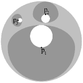
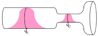
Figure 2. (a) On a disk with three holes, the three shaded regions are the three smallest geodesic balls measuring the three corresponding classes. (b) On a tube, the smallest geodesic ball is centered at $q_{2}$, not $q_{1}$.

2.2. The Optimal Homology Basis

For the $d$-dimensional $\mathbb{Z}_{2}$ homology group whose dimension (Betti number) is $\beta_{d}$, there are $2^{\beta_{d}}-1$ nontrivial homology classes. However, we only need $\beta_{d}$ of them to form a basis. The basis should be chosen wisely so that we can easily distinguish important homology classes from noise. See Figure 1 for an example. There are $2^{3}-1=7$ nontrivial homology classes; we need three of them to form a basis. We would prefer to choose $\{[z_{1}],[z_{2}],[z_{3}]\}$ as a basis, rather than $\{[z_{1}]+[z_{2}]+[z_{3}],[z_{2}]+[z_{3}],[z_{3}]\}$. The former indicates that there is one big cycle in the topological space, whereas the latter gives the impression of three large classes.

In keeping with this intuition, the optimal homology basis is defined as follows.

Definition 2.2.

The optimal homology basis is the basis for the homology group whose elements’ size have the minimal sum, formally,

$$\mathcal{H}_{d}=\operatorname*{argmin}_{\{h_{1},...,h_{\beta_{d}}\}}\sum_{i=1}^{\beta_{d}}S(h_{i}),s.t.\dim(\{h_{1},...,h_{\beta_{d}}\})=\beta_{d}.$$

This definition guarantees that large homology classes appear as few times as possible in the optimal homology basis. In Figure 1, the optimal basis will be $\{[z_{1}],[z_{2}],[z_{3}]\}$, which has only one large class.

For each class in the basis, we need a cycle representing it. As we has shown, $B_{min}(h)$, the smallest geodesic ball carrying $h$, carries at least one cycle of $h$. We localize each class in the optimal basis by its localized-cycles, which are cycles of $h$ carried by $B_{min}(h)$. This is a fair choice because it is consistent to the size measure of $h$ and it is computable in polynomial time. See Section 5 for further discussions.

3. The Algorithm

In this section, we introduce an algorithm to compute the optimal homology basis as defined in Definition 2.2. For each class in the basis, we measure its size, and represent it with one of its localized-cycles. We first introduce an algorithm to compute the smallest homology class, namely, Measure-Smallest($K$). Based on this procedure, we provide the algorithm Measure-All($K$), which computes the optimal homology basis. The algorithm takes $O(\beta_{d}^{4}n^{4})$ time, where $\beta_{d}$ is the Betti number for $d$-dimensional homology classes and $n$ is the cardinality of the input simplicial complex $K$.

Persistent Homology.

Our algorithm uses the persistent homology algorithm. In persistent homology, we filter a topological space with a scalar function, and capture the birth and death times of homology classes of the sublevel set during the filtration course. Classes with longer persistences are considered important ones. Classes with infinite persistences are called essential homology classes and corresponds to the intrinsic homology classes of the given topological space. Please refer to [12, 20, 6] for theory and algorithms of persistent homology.

3.1. Computing the Smallest Homology Class

The procedure Measure-Smallest($K$) measures and localizes, $h_{min}$, the smallest nontrivial homology class, namely, the one with the smallest size. The output of this procedure will be a pair $(S_{min},z_{min})$, namely, the size and a localized-cycle of $h_{min}$. According to the definitions, this pair is determined by the smallest geodesic ball carrying $h_{min}$, namely, $B_{min}(h_{min})$. We first present the algorithm to compute this ball. Second, we explain how to compute the pair $(S_{min},z_{min})$ from the computed ball.

Procedure Bmin($K$): Computing $B_{min}(h_{min})$.

It is straightforward to see that the ball $B_{min}(h_{min})$ is also the smallest geodesic ball carrying any nontrivial homology class of $K$. It can be computed by computing $B_{p}^{r(p)}$ for all vertices $p$, where $B_{p}^{r(p)}$ is the smallest geodesic ball centered at $p$ which carries any nontrivial homology class. When all the $B_{p}^{r(p)}$’s are computed, we compare their radii, $r(p)$’s, and pick the smallest ball as $B_{min}(h_{min})$.

For each vertex $p$, we compute $B_{p}^{r(p)}$ by applying the persistent homology algorithm to $K$ with the discrete geodesic distance from $p$, $f_{p}$, as the filter function. Note that a geodesic ball $B_{p}^{r}$ is the sublevel set $f_{p}^{-1}(-\infty,r]\subseteq K$. Nontrivial homology classes of $K$ are essential homology classes in the persistent homology algorithm. (In the rest of this paper, we may use “essential homology classes” and “nontrivial homology classes of $K$” interchangable.) Therefore, the birth time of the first essential homology class is $r(p)$, and the subcomplex $f_{p}^{-1}(-\infty,r(p)]$ is $B_{p}^{r(p)}$.

Computing $(S_{min},z_{min})$.

We compute the pair from the computed ball $B_{min}(h_{min})$. For simplicity, we denote $p_{min}$ and $r_{min}$ as the center and radius of the ball. According to the definition, $r_{min}$ is exactly the size of $h_{min}$, $S_{min}$. Any nonbounding cycle (a cycle that is not a boundary) carried by $B_{min}(h_{min})$ is a localized-cycle of $h_{min}$. We first computes a basis for all cycles carried by $B_{min}(h_{min})$, using a reduction algorithm. Next, elements in this basis are checked one by one until we find one which is nounbounding in $K$. This checking uses the algorithm of Wiedemann[18] for rank computation of sparse matrices over $\mathbb{Z}_{2}$ field.

3.2. Computing the Optimal Homology Basis

In this section, we present the algorithm for computing the optimal homology basis defined in Definition 2.2, namely, $\mathcal{H}_{d}$. We first show that the optimal homology basis can be computed in a greedy manner. Second, we introduce an efficient greedy algorithm.

3.2.1. Computing $\mathcal{H}_{d}$ in a Greedy Manner

Recall that the optimal homology basis is the basis for the homology group whose elements’ size have the minimal sum. We use matroid theory [9] to show that we can compute the optimal homology basis with a greedy method. Let $H$ be the set of nontrivial $d$-dimensional homology classes (i.e. the homology group minus the trivial class). Let $L$ be the family of sets of linearly independent nontrivial homology classes. Then we have the following theorem, whose proof is omitted due to space limitations. The same result has been mentioned in [14].

Theorem 3.1.

The pair $(H,L)$ is a matroid when $\beta_{d}>0$.

We construct a weighted matroid by assigning each nontrivial homology class its size as the weight. This weight function is strictly positive because a nontrivial homology class can not be carried by a geodesic ball with radius zero. According to matroid theory, we can compute the optimal homology basis with a naive greedy method: check the smallest nontrivial homology classes one by one, until $\beta_{d}$ linearly independent ones are collected. The collected $\beta_{d}$ classes $\{h_{i_{1}},h_{i_{2}},...,h_{i_{\beta_{d}}}\}$ form the optimal homology basis $\mathcal{H}_{d}$. (Note that the $h$’s are ordered by size, i.e. $S(h_{i_{k}})\leq S(h_{i_{k+1}})$.) However, this method is exponential in $\beta_{d}$. We need a better solution.

3.2.2. Computing $\mathcal{H}_{d}$ with a Sealing Technique

In this section, we introduce a polynomial greedy algorithm for computing $\mathcal{H}_{d}$. Instead of computing the smallest classes one by one, our algorithm uses a sealing technique and takes time polynomial in $\beta_{d}$. Intuitively, when the smallest $l$ classes in $\mathcal{H}_{d}$ are picked, we make them trivial by adding new simplices to the given complex. In the augmented complex, any linear combinations of these picked classes becomes trivial, and the smallest nontrivial class is the $(l+1)$’th one in $\mathcal{H}_{d}$.

The algorithm starts by measuring and localizing the smallest homology class of the given simplicial complex $K$ (using the procedure Measure-Smallest($K$) introduced in Section 3.1), which is also the first class we choose for $\mathcal{H}_{d}$. We make this class trivial by sealing one of its cycles – i.e. the localized-cycle we computed – with new simplices. Next, we measure and localize the smallest homology class of the augmented simplicial complex $K^{\prime}$. This class is the second smallest homology class in $\mathcal{H}_{d}$. We make this class trivial again and proceed for the third smallest class in $\mathcal{H}_{d}$. This process is repeated for $\beta_{d}$ rounds, yielding $\mathcal{H}_{d}$.

We make a homology class trivial by sealing the class’s localized-cycle, which we have computed. To seal this cycle $z$, we add (a) a new vertex $v$; (b) a $(d+1)$-simplex for each $d$-simplex of $z$, with vertex set equal to the vertex set of the $d$-simplex together with $v$; (c) all of the faces of these new simplices. In Figure 3 and 3, a $1$-cycle with four edges, $z_{1}$, is sealed up with one new vertex, four new triangles and four new edges.

It is essential to make sure the new simplices does not influence our measurement. We assign the new vertices $+\infty$ geodesic distance from any vertex in the original complex $K$. Furthermore, in the procedure Measure-Smallest($K^{\prime}$), we will not consider any geodesic ball centered at these new vertices. In other words, the geodesic distance from these new vertices will never be used as a filter function. Whenever we run the persistent homology algorithm, all of the new simplices have $+\infty$ filter function values, formally, $f_{p}(\sigma)=+\infty$ for all $p\in\operatorname*{vert}(K)$ and $\sigma\in K^{\prime}\backslash K$.

The algorithm is illustrated in Figure 3 and 3. The 4-edge cycle, $z_{1}$, and the 8-edge cycle, $z_{2}$, are the localized-cycles of the smallest and the second smallest homology classes ($S([z_{1}])=2$,$S([z_{2}])=4$). The nonbounding cycle $z_{3}=z_{1}+z_{2}$ corresponds to the largest nontrivial homology class $[z_{3}]=[z_{1}]+[z_{2}]$ ($S([z_{3}])=5$). After the first round, we choose $[z_{1}]$ as the smallest class in $\mathcal{H}_{1}$. Next, we destroy $[z_{1}]$ by sealing $z_{1}$, which yields the augmented complex $K^{\prime}$. This time, we choose $[z_{2}]$, giving $\mathcal{H}_{1}=\{[z_{1}],[z_{2}]\}$.

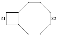
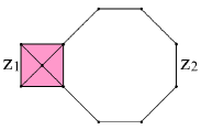
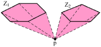
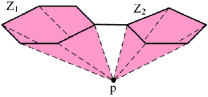
Figure 3. (a,b) the original complex $K$ and the augmented complex $K^{\prime}$ after destroying the smallest class, $[z_{1}]$. (c) If the original complex $K$ consists of the two cycles $z_{1}$ and $z_{2}$, destroying a larger class $[z_{1}]+[z_{2}]$ will make all other classes trivial too. (d) The original complex $K$ consists of the two cycles and an edge connecting them. Destroying $[z_{1}]+[z_{2}]$ will make all other classes trivial and create a new class.

Correctness.

We prove in Theorem 3.3 the correctness of our greedy method. We begin by proving a lemma that destroying the smallest nontrivial class will neither destroy any other classes nor create any new classes. Please note that this is not a trivial result. The lemma does not hold if we seal an arbitrary class instead of the smallest one. See Figure 3 and 3 for examples. Our proof is based on the assumption that the smallest nontrivial class $h_{min}$ is the only one carried by $B_{min}(h_{min})$.

Lemma 3.2.

Given a simplicial complex $K$, if we seal its smallest homology class $h_{min}(K)$, any other nontrivial homology class of $K$, $h$, is still nontrivial in the augmented simplicial complex $K^{\prime}$. In other words, any cycle of $h$ is still nonbounding in $K^{\prime}$.

This lemma leads to the correctness of our algorithm, namely, Theorem 3.3. We prove this theorem by showing that the procedure Measure-All($K$) produces the same result as the naive greedy algorithm.

Theorem 3.3.

The procedure Measure-All($K$) computes $\mathcal{H}_{d}$.

4. An Improvement Using Finite Field Linear Algebra

In this section, we present an improvement on the algorithm presented in the previous section, more specifically, an improvement on computing the smallest geodesic ball carrying any nontrivial class (the procedure Bmin). The idea is based on the finite field linear algebra behind the homology.

We first observe that for neighboring vertices, $p_{1}$ and $p_{2}$, the birth times of the first essential homology class using $f_{p_{1}}$ and $f_{p_{2}}$ as filter functions are close (Theorem 4.1). This observation suggests that for each $p$, instead of computing $B_{p}^{r(p)}$, we may just test whether the geodesic ball centered at $p$ with a certain radius carries any essential homology class. Second, with some algebraic insight, we reduce the problem of testing whether a geodesic ball carries any essential homology class to the problem of comparing dimensions of two vector spaces. Furthermore, we use Theorem 4.3 to reduce the problem to rank computations of sparse matrices on the $\mathbb{Z}_{2}$ field, for which we have ready tools from the literature. In what follows, we assume that $K$ has a single component; multiple components can be accommodated with a simple modification.

Complexity.

In doing so, we improve the complexity to $O(\beta_{d}^{4}n^{3}\log^{2}n)$. More detailed complexity analysis is omitted due to space limitations.

Next, we present details of the improvement. In Section 4.1, we prove Theorem 4.1 and provide details of the improved algorithm. In Section 4.2, we explain how to test whether a certain subcomplex carries any essential homology class of $K$. For convenience, in this section, we use “carrying nonbounding cycles” and “carrying essential homology classes” interchangeably, because a geodesic ball carries essential homology classes of $K$ if and only if it carries nonbounding cycles of $K$.

4.1. The Stability of Persistence Leads to An Improvement

Cohen-Steiner et al.[6] proved that the change, suitably defined, of the persistence of homology classes is bounded by the changes of the filter functions. Since the filter functions of two neighboring vertices, $f_{p_{1}}$ and $f_{p_{2}}$, are close to each other, the birth times of the first nonbounding cycles in both filters are close as well. This leads to Theorem 4.1. A simple proof is provided.

Theorem 4.1.

If two vertices $p_{1}$ and $p_{2}$ are neighbors, the birth times of the first nonbounding cycles for filter functions $f_{p_{1}}$ and $f_{p_{2}}$ differ by no more than 1.

Proof 4.2.

$p_{1}$ and $p_{2}$ are neighbors implies that for any point $q$, $f_{p_{2}}(q)\leq f_{p_{2}}(p_{1})+f_{p_{1}}(q)=1+f_{p_{1}}(q)$, in which the inequality follows the triangular inequality. Therefore, $B_{p_{1}}^{r(p_{1})}$ is a subset of $B_{p_{2}}^{r(p_{1})+1}$. The former carries nonbounding cycles implies that the latter does too, and thus $r(p_{2})\leq r(p_{1})+1$. Similarly, we have $r(p_{1})\leq r(p_{2})+1$. ∎

This theorem suggests a way to avoid computing $B_{p}^{r(p)}$ for all $p\in\operatorname*{vert}(K)$ in the procedure Bmin. Since our objective is to find the minimum of the $r(p)$’s, we do a breadth-first search through all the vertices with global variables $r_{min}$ and $p_{min}$ recording the smallest $r(p)$ we have found and its corresponding center $p$, respectively. We start by applying the persistent homology algorithm on $K$ with filter function $f_{p_{0}}$, where $p_{0}$ is an arbitrary vertex of $K$. Initialize $r_{min}$ as the birth time of the first nonbounding cycle of $K$, $r(p_{0})$, and $p_{min}$ as $p_{0}$. Next, we do a breadth-first search through the rest vertices. For each vertex $p_{i},i\neq 0$, there is a neighbor $p_{j}$ we have visited (the parent vertex of $p_{i}$ in the breath-first search tree). We know that $r(p_{j})\geq r_{min}$ and $r(p_{i})\geq r(p_{j})-1$ (Theorem 4.1). Therefore, $r(p_{i})\geq r_{min}-1$. We only need to test whether the geodesic ball $B_{p_{i}}^{r_{min}-1}$ carries any nonbounding cycle of $K$. If so, $r_{min}$ is decremented by one, and $p_{min}$ is updated to $p_{i}$. After all vertices are visited, $p_{min}$ and $r_{min}$ give us the ball we want.

However, testing whether the subcomplex $B_{p_{i}}^{r_{min}-1}$ carries any nonbounding cycle of $K$ is not as easy as computing nonbounding cycles of the subcomplex. A nonbounding cycle of $B_{p}^{r_{min}-1}$ may not be nonbounding in $K$ as we require. For example, in Figure 4 and 4, the simplicial complex $K$ is a torus with a tail. The pink geodesic ball in the first figure does not carry any nonbounding cycle of $K$, although it carries its own nonbounding cycles. The geodesic ball in the second figure is the one that carries nonbounding cycles of $K$. Therefore, we need algebraic tools to distinguish nonbounding cycles of $K$ from those of the subcomplex $B_{p_{i}}^{r_{min}-1}$.

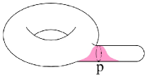
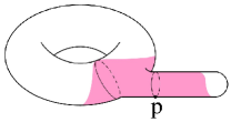
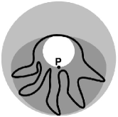
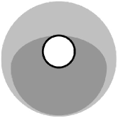
Figure 4. (a,b) In a torus with a tail, only the ball in the second figure carries nonbounding cycles of $K$, although in both figures the balls have nontrivial topology. (c,d) The cycles with the minimal radius and the minimal diameter, $z_{r}$ and $z_{d}$ (Used in Section 5).

4.2. Procedure Contain-Nonbounding-Cycle: Testing Whether a Subcomplex Carries Nonbounding Cycles of $K$

In this section, we present the procedure for testing whether a subcomplex $K_{0}$ carries any nonbounding cycle of $K$. A chain in $K_{0}$ is a cycle if and only if it is a cycle of $K$. However, solely from $K_{0}$, we are not able to tell whether a cycle carried by $K_{0}$ bounds or not in $K$. Instead, we write the set of cycles of $K$ carried by $K_{0}$, $\mathsf{Z}_{d}^{K_{0}}(K)$, and the set of boundaries of $K$ carried by $K_{0}$, $\mathsf{B}_{d}^{K_{0}}(K)$, as sets of linear combinations with certain constraints. Consequently, we are able to test whether any cycle carried by $K_{0}$ is nonbounding in $K$ by comparing their dimensions. Formally, we define $\mathsf{B}_{d}^{K_{0}}(K)=\mathsf{B}_{d}(K)\cap\mathsf{C}_{d}(K_{0})$ and $\mathsf{Z}_{d}^{K_{0}}(K)=\mathsf{Z}_{d}(K)\cap\mathsf{C}_{d}(K_{0})$.

Let $\hat{H}_{d}=[z_{1},...,z_{\beta_{d}}]$ be the matrix whose column vectors are arbitrary $\beta_{d}$ nonbounding cycles of $K$ which are not homologous to each other. The boundary group and the cycle group of $K$ are column spaces of the matrices $\partial_{d+1}$ and $\hat{Z}_{d}=[\partial_{d+1},\hat{H}_{d}]$, respectively. Using finite field linear algebra, we have the following theorem, whose proof is omitted due to space limitations.

Theorem 4.3.

$K_{0}$ carries nonbounding cycles of $K$ if and only if

$$\operatorname*{rank}(\hat{Z}_{d}^{K\backslash K_{0}})-\operatorname*{rank}(\partial_{d+1}^{K\backslash K_{0}})\neq\beta_{d}.$$

where $\partial_{d+1}^{i}$ and $\hat{Z}_{d}^{i}$ are the $i$-th rows of the matrices $\partial_{d+1}$ and $\hat{Z}_{d}$, respectively.

We use the algorithm of Wiedemann[18] for the rank computation. In our algorithm, the boundary matrix $\partial_{d+1}$ is given. The matrix $\hat{H}_{d}$ can be precomputed as follows. We perform a column reduction on the boundary matrix $\partial_{d}$ to compute a basis for the cycle group $\mathsf{Z}_{d}(K)$. We check elements in this basis one by one until we collect $\beta_{d}$ of them forming $\hat{H}_{d}$. For each cycle $z$ in this cycle basis, we check whether $z$ is linearly independent of the $d$-boundaries and the nonbounding cycles we have already chosen. More details are omitted due to space limitations.

5. Localizing Classes

In this section, we address the localization problem. We formalize the localization problem as a combinatorial optimization problem: Given a simplcial complex $K$, compute the representative cycle of a given homology class minimizing a certain objective function. Formally, given an objective function defined on all the cycles, $\operatorname*{cost}:\mathsf{Z}_{d}(K)\to\mathbb{R}$, we want to localize a given class with its optimally localized cycle, $z_{opt}(h)=\operatorname*{argmin}_{z\in h}\operatorname*{cost}(z)$. In general, we assume the class $h$ is given by one of its representative cycles, $z_{0}$.

We explore three options of the objective function $\operatorname*{cost}(z)$, i.e. the volume, diameter and radius of a given cycle $z$. We show that the cycle with the minimal volume and the cycle with the minimal diameter are NP-hard to compute. The cycle with the minimal radius, which is the localized-cycle we defined and computed in previous sections, is a fair choice. Due to space limitations, we omit proofs of theorems in this section.

Definition 5.1 (Volume).

The volume of $z$ is the number of its simplices, $\operatorname*{vol}(z)=\operatorname*{card}(z)$.

For example, the volume of a 1-dimensional cycle, a 2-dimensional cycle and a 3-dimensional cycle are the numbers of their edges, triangles and tetrahedra, respectively. A cycle with the smallest volume, denoted as $z_{v}$, is consistent to a “well-localized” cycle in intuition. Its 1-dimensional version, the shortest cycle of a class, has been studied by researchers [14, 19, 11]. However, we prove in Theorem 5.2 that computing $z_{v}$ of $h$ is NP-hard. The proof is by reduction from the NP-hard problem MAX-2SAT-B [17]. More generally, we can extend the the volume to be the sum of the weights assigned to simplices of the cycle, given an arbitrary weight function defined on all the simplices of $K$. The corresponding smallest cycle is still NP-hard to compute.

Theorem 5.2.

Computing $z_{v}$ for a given $h$ is NP-hard.

When it is NP-hard to compute $z_{v}$, one may resort to the geodesic distance between elements of $z$. The second choice of the objective function is the diameter.

Definition 5.3 (Diameter).

The diameter of a cycle is the diameter of its vertex set, $\operatorname*{diam}(z)=\operatorname*{diam}(\operatorname*{vert}(z))$, in which the diameter of a set of vertices is the maximal geodesic distance between them, formally, $\operatorname*{diam}(S)=\max_{p,q\in S}\operatorname*{dist}(p,q)$.

Intuitively, a representative cycle of $h$ with the minimal diameter, denoted $z_{d}$, is the cycle whose vertices are as close to each other as possible. The intuition will be further illustrated by comparison against the radius criterion. We prove in Theorem 5.4 that computing $z_{d}$ of $h$ is NP-hard, by reduction from the NP-hard Multiple-Choice Cover Problem (MCCP) of Arkin and Hassin [2].

Theorem 5.4.

Computing $z_{d}$ for a given $h$ is NP-hard.

The third option of the objective function is the radius.

Definition 5.5 (Radius).

The radius of a cycle is the radius of the smallest geodesic ball carrying it, formally, $\operatorname*{rad}(z)=\min_{p\in\operatorname*{vert}(K)}\max_{q\in\operatorname*{vert}(z)}\operatorname*{dist}(p,q)$, where $\operatorname*{vert}(K)$ and $\operatorname*{vert}(z)$ are the sets of vertices of the given simplicial complex $K$ and the cycle $z$, respectively.

The representative cycle with the minimal radius, denoted as $z_{r}$, is the same as the localized-cycle defined and computed in previous sections. Intuitively, $z_{r}$ is the cycle whose vertices are as close to a vertex of $K$ as possible. However, $z_{r}$ may not necessarily be localized in intuition. It may wiggle a lot while still being carried by the smallest geodesic ball carrying the class. See Figure 4, in which we localize the only nontrivial homology class of an annulus (the light gray area). The dark gray area is the smallest geodesic ball carrying the class, whose center is $p$. Besides, the cycle with the minimal diameter (Figure 4) avoids this wiggling problem and is concise in intuition. This in turn justifies the choice of diameter. We can prove that $z_{r}$ can be computed in polynomial time and is a 2-approximation of $z_{d}$.

Theorem 5.6.

We can compute $z_{r}$ in polynomial time.

Theorem 5.7.

$\operatorname*{diam}(z_{r})\leq 2\operatorname*{diam}(z_{d})$.

This bound is a tight bound. In Figure 4 and 4, the diameter of the cycle $z_{r}$ is twice of the radius of the dark gray geodesic ball. The diameter of the cycle $z_{d}$ is the same as the radius of the ball. We have $\operatorname*{diam}(z_{r})=2\operatorname*{diam}(z_{d})$.

References

- [1] P. K. Agarwal, H. Edelsbrunner, J. Harer, and Y. Wang. Extreme elevation on a 2-manifold. Discrete & Computational Geometry, 36:553–572, 2006.
- [2] E. M. Arkin and R. Hassin. Minimum-diameter covering problems. Networks, 36(3):147–155, 2000.
- [3] G. Carlsson. Persistent homology and the analysis of high dimensional data. Symposium on the Geometry of Very Large Data Sets, Febrary 2005. Fields Institute for Research in Mathematical Sciences.
- [4] G. Carlsson, T. Ishkhanov, V. de Silva, and L. J. Guibas. Persistence barcodes for shapes. International Journal of Shape Modeling, 11(2):149–188, 2005.
- [5] C. Carner, M. Jin, X. Gu, and H. Qin. Topology-driven surface mappings with robust feature alignment. In IEEE Visualization, p. 69, 2005.
- [6] D. Cohen-Steiner, H. Edelsbrunner, and J. Harer. Stability of persistence diagrams. Discrete & Computational Geometry, 37:103–120, 2007.
- [7] D. Cohen-Steiner, H. Edelsbrunner, and J. Harer. Extending persistent homology using Poincaré and Lefschetz duality. Foundations of Computational Mathematics, to appear.
- [8] D. Cohen-Steiner, H. Edelsbrunner, and D. Morozov. Vines and vineyards by updating persistence in linear time. In Symposium on Computational Geometry, pp. 119–126, 2006.
- [9] T. H. Cormen, C. E. Leiserson, R. L. Rivest, and C. Stein. Introduction to Algorithms. MIT Press, 2001.
- [10] V. de Silva and R. Ghrist. Coverage in sensor networks via persistent homology. Algebraic & Geometric Topology, 2006.
- [11] T. K. Dey, K. Li, and J. Sun. On computing handle and tunnel loops. In IEEE Proc. NASAGEM, 2007.
- [12] H. Edelsbrunner, D. Letscher, and A. Zomorodian. Topological persistence and simplification. Discrete & Computational Geometry, 28(4):511–533, 2002.
- [13] J. Erickson and S. Har-Peled. Optimally cutting a surface into a disk. Discrete & Computational Geometry, 31(1):37–59, 2004.
- [14] J. Erickson and K. Whittlesey. Greedy optimal homotopy and homology generators. In SODA, pp. 1038–1046, 2005.
- [15] R. Ghrist. Barcodes: the persistent topology of data. Amer. Math. Soc Current Events Bulletin.
- [16] J. R. Munkres. Elements of Algebraic Topology. Addison-Wesley, Redwook City, California, 1984.
- [17] C. Papadimitriou and M. Yannakakis. Optimization, approximation, and complexity classes. In Proc. 20th ACM Symposium on Theory of computing, pp. 229–234, New York, NY, USA, 1988. ACM Press.
- [18] D. H. Wiedemann. Solving sparse linear equations over finite fields. IEEE Transactions on Information Theory, 32(1):54–62, 1986.
- [19] Z. J. Wood, H. Hoppe, M. Desbrun, and P. Schröder. Removing excess topology from isosurfaces. ACM Trans. Graph., 23(2):190–208, 2004.
- [20] A. Zomorodian and G. Carlsson. Computing persistent homology. Discrete & Computational Geometry, 33(2):249–274, 2005.
- [21] A. Zomorodian and G. Carlsson. Localized homology. In Shape Modeling International, pp. 189–198, 2007.