title

Geometric Set Cover and Hitting Sets
for Polytopes in $\mathbb{R}^{3}$

Abstract.

Suppose we are given a finite set of points $P$ in $\mathbb{R}^{3}$ and a collection of polytopes $\mathcal{T}$ that are all translates of the same polytope $T$. We consider two problems in this paper. The first is the set cover problem where we want to select a minimal number of polytopes from the collection $\mathcal{T}$ such that their union covers all input points $P$. The second problem that we consider is finding a hitting set for the set of polytopes $\mathcal{T}$, that is, we want to select a minimal number of points from the input points $P$ such that every given polytope is hit by at least one point.

We give the first constant-factor approximation algorithms for both problems. We achieve this by providing an epsilon-net for translates of a polytope in $\mathbb{R}^{3}$ of size $O(\frac{1}{\epsilon})$.

2008479-490Bordeaux 479

Introduction

Suppose we are given a set of $n$ points $P$ in $\mathbb{R}^{3}$ and a collection of polytopes $\mathcal{T}$ that are all translates of the same polytope $T$. We consider two problems in this paper. The first is the set cover problem where we want to select a minimal number of polytopes from the collection $\mathcal{T}$ such that their union covers all input points $P$. The second problem that we consider is finding a hitting set for the set of polytopes $\mathcal{T}$, that is, we want to select a minimal number of points from the input points $P$ such that every given polytope is hit by at least one point.

Both problems, the set cover problem and the hitting set problem which are in fact dual to each other are very fundamental problems and have been studied intensively. In a more general setting, where the sets could be arbitrary subsets, both problems are known to be NP-hard, in fact they are even hard to approximate within $o(\log n)$ [11]. Even when the sets are induced by geometric objects it is widely believed that the corresponding set cover problem as well as the hitting set problem are NP-hard. Several geometric versions of these problems were even proven to be hard to approximate. Hence, we are looking for algorithms that approximate both problems. We give the first constant-factor approximation algorithms for the set cover problem and the hitting set problem for translates of a polytope in $\mathbb{R}^{3}$. The central idea to our approximation algorithms are small epsilon-nets.

A set of elements $P$ (also called points) along with a collection $\mathcal{T}$ of subsets of $P$ (also called ranges) is in general called a set system $(P,\mathcal{T})$ and for geometric settings also known as range spaces. One essential characteristic of these set systems is the Vapnik-Chervonenkis dimension, or VC-dimension [17]. The VC-dimension is the cardinality of the largest subset $A\subseteq P$ for which $\{T\cap A:T\in\mathcal{T}\}$ is the powerset of $A$. If the set $A$ is finite, we say that the set system $(P,\mathcal{T})$ has bounded VC-dimension, otherwise we say the VC-dimension of $(P,\mathcal{T})$ is unbounded. For instance, the set system induced by translates of a polytope has VC-dimension three as well as the set system induced by halfspaces in $\mathbb{R}^{2}$. A set $N\subseteq P$ is called an epsilon-net for a given set system $(P,\mathcal{T})$ if $N\cap T\neq\emptyset$ for every subset $T\in\mathcal{T}$ for which $\|T\|\geq\epsilon\cdot\|P\|$. In other words, an epsilon-net is a hitting set for all subsets $T\in\mathcal{T}$ whose cardinality is an $\epsilon$-fraction of the cardinality of the input point set $P$.

It is known that there exist epsilon-nets of size $O\left(\frac{d}{\epsilon}\log\frac{d}{\epsilon}\right)$ for any set system of VC-dimension $d$ [2, 10]. This bound is in fact tight for arbitrary set systems as there exist set systems that do not admit epsilon-nets of size less than this bound [16]. Such an epsilon-net can be simply found by random sampling [12].

However, for special set systems that are induced by geometric objects there do exist epsilon-nets of smaller size, namely of size $O(\frac{1}{\epsilon})$. It has been shown by Pach and Woeginger [16] that halfspaces in $\mathbb{R}^{2}$ and translates of polytopes in $\mathbb{R}^{2}$ admit epsilon-net of size $O(\frac{1}{\epsilon})$. Matoušek et al. [14] gave an algorithm for computing small epsilon-nets for pseudo-disks in $\mathbb{R}^{2}$ and halfspaces in $\mathbb{R}^{3}$. The result for halfspaces in $\mathbb{R}^{3}$ also follows from a more general statement by Matoušek [13].

Among other reasons for finding epsilon-nets of small size is the fact that an epsilon-net of size $g(\epsilon)$ immediately implies an approximation algorithm for the corresponding hitting set with approximation guarantee of $O(g(1/c)/c)$, where $c$ denotes the optimal solution to the hitting set [15]. This means, that for arbitrary set systems of fixed VC-dimension we have an algorithm for the hitting set problem with approximation $O(\log c)$. And for set systems that admit epsilon-nets of size $O(1/\epsilon)$ we get an approximation algorithm to the hitting set problem with constant approximation guarantee.

Clarkson and Varadarajan [5] developed a technique that connects the complexity of a union of geometric objects to the size of the epsilon-net for the dual set system. Using this result, they are able to develop, among other approximation algorithms for geometric objects in $\mathbb{R}^{2}$, a constant-factor approximation algorithm for the set cover problem induced by translates of unit cubes in $\mathbb{R}^{3}$.

We extend their result to not only the set cover problem but also the hitting set problem for arbitrary translates of a polytope in $\mathbb{R}^{3}$. We do not require the polytope to be convex or fat. This is the first constant-factor approximation algorithm for these two problems. We achieve this by giving an epsilon-net for translates of a polytope in $\mathbb{R}^{3}$ of size $O(\frac{1}{\epsilon})$. We reduce the problem of finding epsilon-nets for translates of a polytope to a family of non-piercing objects in $\mathbb{R}^{2}$ and then generalize the epsilon-net finder for pseudo-disks of Matoušek et al. [14] to our setting.

The set cover problem which is studied by Hochbaum and Maass [9] where one is allowed to move the objects is fundamentally different. They give a PTAS for their problem.

1. Small Epsilon-Nets for Polytopes in $\mathbb{R}^{3}$

Let $P$ be a set of $n$ points in $\mathbb{R}^{3}$ and let $\mathcal{T}$ be a family of polytopes that are all translates of the same bounded polytope $T_{0}$. We want to find a set of polytopes of minimal cardinality among the collection $\mathcal{T}$ that covers all input points $P$. First, we find a small epsilon-net for this set system and use this later for the constant-factor approximation of the hitting set problem. Finally, we show how this then can be translated into a solution for the set cover problem.

Throughout this paper we denote by $T$ the polytope as well as the subset of points from $P$ that $T$ covers and by $\mathcal{T}$ the family of polytopes as well as the corresponding family of subsets of $P$. This will make the paper easier to read and it will be clear from the context whether we talk about the geometric object or the corresponding set of points.

1.1. From Polytopes in $\mathbb{R}^{3}$ to Non-Piercing Objects in $\mathbb{R}^{2}$

So given such a set system $(P,\mathcal{T})$ we want to find an epsilon-net for it, i.e. we are looking for a set $N\subseteq P$ such that every subset of points $T\in\mathcal{T}$ with $\|T\|\geq\epsilon\cdot\|P\|$ is stabbed by at least one point from $N$.

We can cut the polytope $T$ into, lets say $k$ polytopes $T_{1},T_{2},\ldots,T_{k}$. If the polytope $T$ contains $\epsilon n$ input points then one of the polytopes $T_{1},T_{2},\ldots,T_{k}$ must contain at least $\frac{\epsilon}{k}\cdot n$ input points. Hence, in order to find an $\epsilon$-net for the set system $(P,\mathcal{T})$ induced by translates of $T$, it suffices to find $\frac{\epsilon}{k}$-net for the set systems induced by the translates of $T_{1},T_{2},\ldots,T_{k}$.

Following this reasoning we can reduce our problem for finding an epsilon-net for the set system induced by translates of arbitrary polytopes to translates of convex polytopes by cutting the possibly non-convex polytope into a set of convex polytopes. Note that the number of these convex polytopes only depends on the polytope $T$ and hence is constant for fixed $T$.

Wlog. let $T$ be from now on a convex polytope. We can place a cubical grid onto the space $\mathbb{R}^{3}$ such that for any translate of $T$ every cubical grid cell contains at most vertex of $T$. This can be achieved by making the grid fine enough. Clearly, the maximal number $t$ of grid cells that can be intersected by $T$ is bounded and only depends on $T$. Again, if $T$ contains $\epsilon n$ input points then at least one of the cells must contain at least $\frac{\epsilon}{t}\cdot n$ of the input points. Hence, we can restrict ourselves to finding epsilon-nets for translates of triangular cones where all input points lie in a cube in $\mathbb{R}^{3}$. This just adds a multiplicative constant to the size of the final epsilon-net.

The case when the cubical cell only contains a halfspace or the intersection of two halfspaces can be either seen as a special case of a cone or, in fact, be even treated separately in a much simpler way. The case of a translate of a halfspace reduces to a one-dimensional problem an admits an epsilon-net of size 1 and the case of two intersecting halfspaces reduces to a problem on intervals which admits an epsilon-net of size $O(1/\epsilon)$.

In the following we will construct an epsilon-net for the set system $(P,\mathcal{C})$ that is induced by translates of a triangular cone $C$.

Given a cone $C$, we call a set of points $P$ in non-$C$-degenerate position if every translate of $C$ has at most three points of $P$ on its boundary. We can always perturb the input points $P$ in such a way that they are in non-$C$-degenerate position and the collection of subsets of the form $P\cap C_{T}$ where $C_{T}$ is a translate of $C$ does not decrease [6]. Hence, we can restrict ourselves on non-$C$-degenerate set of points $P$.

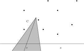
Figure 1. The cone $C$ and its internal ray $r$.

We place a coordinate system such that the input points all have $z$-coordinate greater than $0$ and a ray $r$ emitting from the apex of the cone $C$ and lying entirely in the cone should intersect the plane $z=0$. We refer to such a cone as a cone that opens to the bottom and the ray $r$ as its internal ray. Figure 1 illustrates this setup for the two-dimensional case.

The following two definitions are helpful generalizations the lower envelope.

Given a finite point set $P$ and a triangular cone $C$ that opens to the bottom consider the arrangement of all translates of $C$ that have a point of $P$ on its boundary but no point of $P$ in its interior. The upper set of plane segments that can be seen from above is called the lower envelope of $P$ with respect to cone $C$.

Figure 3 illustrates the definition of the lower envelope in the two-dimensional case. This definition is similar to the definition of alpha-shapes where the cone is replaced by a ball. We call all points that lie on the lower envelope with respect to cone $C$ lower envelope points and denote this set by $L$.

Figure 2. The lower envelope with respect to cone $C$, the corresponding cones are drawn dotted.

Figure 3. The flattened lower envelope with respect to cone $C$, lower envelope is drawn dotted.

Let $C$ be a triangular cone that opens to the bottom and let $P\subseteq\mathbb{R}^{3}$ be a finite set of points in non-$\mathcal{C}$-degenerate position. Let $C^{\prime}$ be a cone that is flatter that $C$ by small $\delta$ and such that it contains $C$ and the combinatorial structure of $P$ and $C^{\prime}$ is the same as for $P$ and $C$. See figure 3 for an illustration. Then, the lower envelope of $P$ with respect to $C^{\prime}$ is called the flattened lower envelope of $P$ with respect to cone $C$. Such a cone $C^{\prime}$ always exists for a finite point set that is in non-$\mathcal{C}$-degenerate position. From now on we will abbreviate the term lower envelope with respect to cone $C$ by lower envelope since we will throughout this paper only talk about the same cone $C$. The flattened lower envelope can be basically seen as a slightly flattened version of the lower envelope.

The next lemma shows that we can reduce the problem of finding an epsilon-net with respect to cones of arbitrary point sets to lower envelope points.

Lemma 1.1.

If for every finite point set $P^{\prime}\subseteq\mathbb{R}^{3}$ of lower envelope points in non-$C$-degenerate position there exists an epsilon-net with respect to translates of a cone $C$ of size $s(\epsilon)$ then there exists an epsilon-net with respect to translates of a cone $C$ of size $3s(\epsilon)$ for every finite point set $P\subseteq\mathbb{R}^{3}$ in non-$C$-degenerate position.

Figure 4. The projection of points onto flattened lower envelope.

.

Proof 1.2.

Let $P\subseteq\mathbb{R}^{3}$ be such a finite point set in non-$\mathcal{C}$-degenerate position and let $C$ denote the cone. Let $L$ denote the set of lower envelope points. Let $\bar{L}=P\setminus L$ be the set of all non-lower envelope points. We project all non-lower envelope points $\bar{L}$ along the internal ray $r$ of cone $C$ onto the flattened lower envelope (cf. figure 4). We denote the projection of a point $p$ by $p^{\prime}$. Let $P^{\prime}$ be union of the projected points and $L$. Clearly, $P^{\prime}$ is a set of lower envelope points in non-$C$-degenerate position.

Suppose we have an epsilon-net $N^{\prime}$ for this point set $P^{\prime}$. From this epsilon-net $N^{\prime}$ we will construct an epsilon-net $N$ for the original point set $P$. If a point from the set $L$ is in the epsilon-net $N^{\prime}$, we also add it to the epsilon-net $N$ for $P$. If however, a projected point $p^{\prime}$ is in $N^{\prime}$ then we add to $N$ the three points $p_{1},p_{2}$ and $p_{3}$ from the lower envelope $L$ that determine the cone $C$ on whose boundary also $p^{\prime}$ lies. Note that whenever an arbitrary cone contains the point $p^{\prime}$ then it has to contain one of the three points $p_{1},p_{2}$ or $p_{3}$.

We have the following two properties:

1. If a cone contains at least $\epsilon n$ points from the set $P$ then it contains at least $\epsilon n$ points from the set $P^{\prime}$.

2. If a cone contains a point from the epsilon-net $N^{\prime}$ for $P^{\prime}$ then the cone contains a point from the epsilon-net $N$ for $P$.

Both properties prove that the set $N$ is indeed an epsilon-net for $P$.

The preceding lemma assures that we can restrict ourselves on a finite set of lower envelope points in non-$C$-degenerate position. For such a set system we will now construct a corresponding set system of points in the plane and a collection of regions in the plane.

Let $C$ be a cone and let $P^{\prime}$ be a finite set of lower envelope points in non-$C$-degenerate position and let $\mathcal{C}$ be a collection of translates of $C$. We define a projection $\tau$ from the flattened lower envelope onto the plane $z=0$ by projecting each point along the internal ray $r$. Let the projection of all points $p^{\prime}\in P^{\prime}$ which all lie on the be denoted as the set $S$. For each cone of the collection the image of the intersection of the cone with the flattened lower envelope is an object $D\subseteq\mathbb{R}^{2}$ and the family $\mathcal{C}$ of cones induces a family of objects which we will denote by $\mathcal{D}$. Using the flattened lower envelope instead of the lower envelope avoids degeneracy. The intersection of an arbitrary cone with the flattened lower envelope is always a collection of line segments. Furthermore, it makes everything continuous in the sense that if a cone is moved continuously in $\mathbb{R}^{3}$ then the intersection of the cone with the flattened lower envelope moves continuously as well as its image of the projection $\tau$. Note, that $\tau$ is injective.

Analogously, we call a set of points $S\subseteq\mathbb{R}^{2}$ in non-$\mathcal{D}$-degenerate position if every $D\in\mathcal{D}$ has at most three points on its boundary. We have the following lemma:

Lemma 1.3.

If for every finite point set $S\subseteq\mathbb{R}^{2}$ in non-$\mathcal{D}$-degenerate position there exists an epsilon-net with respect to the family of objects $\mathcal{D}$ produced by the projection $\tau$ of size $s(\epsilon)$ then there exists an epsilon-net with respect to cones of size $s(\epsilon)$ for every point set of lower envelope points $P^{\prime}\subseteq\mathbb{R}^{3}$ in non-$\mathcal{C}$-degenerate position.

Proof 1.4.

The proof follows easily from the fact that the image of a cone $C$ under the projection $\tau$ contains exactly those points that are the image of the points that are contained in $C$.

We refer to a cone $C$ as the corresponding cone of the object $D=\tau(C)$. We will prove a few useful properties of the so constructed set system $(S,\mathcal{D})$.

Notice, that the intersection of two triangular cones is again a cone. Furthermore, the intersection of a possibly infinite family of triangular cones is either empty or again a triangular cone since all cones are closed. The intersection of the boundary of a cone with the flattened lower envelope is either empty or a set of line segments that form one simple closed cycle. Hence, the image of a cone under the projection $\tau$ is a closed and connected region whose boundary is a closed and connected cycle.

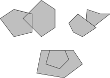
Figure 5. A set of non-piercing objects

.

Definition 1.5.

Two geometric objects(sets) $A\subseteq\mathbb{R}^{2}$ and $B\subseteq\mathbb{R}^{2}$ that are bounded by Jordan curves are said to be non-piercing if the boundary of $A$ and $B$ cross at most twice. A family of geometric objects is called non-piercing if every two objects from this family are non-piercing. See figure 5 for an illustration.

Lemma 1.6.

The projection $\tau$ produces a family $\mathcal{D}$ of non-piercing objects.

Proof 1.7.

Consider two cones $C_{1}$ and $C_{2}$ that intersect each other. If one is contained in the other, i.e. $C_{1}\subseteq C_{2}$ then we are done, as $\tau(C_{1})\subseteq\tau(C_{2})$ and hence their boundaries cannot cross. So if $C_{1}$ and $C_{2}$ intersect and none is subset of the other then the intersection of their boundaries are two rays emitting from the same point. Each of these rays intersects the flattened lower envelope exactly once. Hence, as the projection $\tau$ is injective the boundary of the two images of the cones $C_{1}$ and $C_{2}$ under the projection $\tau$ intersect exactly twice. Thus, the objects are non-piercing.

1.2. Small Epsilon-Nets for Non-Piercing Objects in $\mathbb{R}^{2}$

In this subsection we will derive a few properties of the projection that are necessary to apply the algorithm of Matoušek et al. [14] for finding a small epsilon-net for pseudo-disks. These properties also hold in general for any family of non-piercing objects with the additional property that for any three points there always exists an object that has these three points on its boundary. However the proofs are a bit more involved. Since this does not lie in the scope of this paper, we omit this here and focus only on the special family of non-piercing objects that is produced by the projection described above.

Consider the family of all cones that have $p$ and $q$ on its boundary. The intersection of all these cones is a cone $C_{pq}$ that has $p$ and $q$ on its boundary. Connect $p$ and $q$ by a Jordan curve $E_{pq}$ such that it lies entirely in the cone $C_{pq}$ and on the flattened lower envelope, for instance part of the boundary of $C_{pq}$ that intersects the flattened lower envelope. The image of $E_{pq}$ under the projection $\tau$ is a curve $\tau(E_{pq})$ embedded in the plane.

Let $\mathcal{D}$ be a family of non-piercing objects and let $S\subseteq\mathbb{R}^{2}$ be a finite set of points. We call two points $p,q\in\mathbb{R}^{2}$ $\mathcal{D}$-Delaunay neighbors if there exists an object $D\in\mathcal{D}$ that has $p$ and $q$ on its boundary and no other point of $S$ in its interior. The $\mathcal{D}$-Delaunay graph of $S$, in short $\mathcal{D}$-$\operatorname{DT}(S)$, is the graph that is embedded in the plane, has $S$ as its vertex set and the edges $\tau(E_{pq})$ between all $\mathcal{D}$-Delaunay neighbors $p$ and $q$. Due to the definition of the $\mathcal{D}$-Delaunay edge between two $\mathcal{D}$-Delaunay neighbors $p$ and $q$ it is guaranteed that whenever a object $D\in\mathcal{D}$ contains $p$ as well as $q$ then it also must contain the $\mathcal{D}$-Delaunay edge $\tau(E_{pq})$. In the following we will prove that this $\mathcal{D}$-Delaunay graph is in fact a triangulation of the vertex set $S$.

Lemma 1.8.

The $\mathcal{D}$-Delaunay graph of the given finite point set $S$ in non-$\mathcal{D}$-degenerate position is a triangulation.

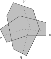
Figure 6. Two intersecting $\mathcal{D}$-Delaunay edges and their defining objects

.

Proof 1.9.

First, we will prove that $\mathcal{D}$-$\operatorname{DT}(S)$ is planar. Suppose otherwise, i.e. two edges $\tau(E_{pq})$ and $\tau(E_{rs})$ intersect each other in the plane. Since the cone $C_{pq}$ does not have any point in its interior and $C_{rs}$ also does not have any point in its interior and since each of these cones has at most $3$ points on its boundary the objects $\tau(C_{pq})$ and $\tau(C_{rs})$ would have to pierce each other, see figure 6 for an illustration. Here, it is actually essential, that the set $S$ is in non-$\mathcal{D}$-degenerate position. Thus, the graph is planar.

The graph $\mathcal{D}$-$\operatorname{DT}(S)$ itself consists of an outer face which is defined by cones of the lower envelope that have at most 2 points on their boundary and all other faces are triangles defined by the cones of the lower envelope that have exactly three points on its boundary. Suppose an inner face $F$ is not bounded by a triangle. Then, one can place the apex of a cone in such a way onto the flattened lower envelope such that its image under the projection $\tau$ is a point which lies inside this face $F$. By moving the cone upward one can ensure that the cone will finally have three points on its boundary whose image under the projection $\tau$ are three vertices of the face $F$ but no point in its interior. Hence, the face $F$ must be bounded by a triangle. Hence, $\mathcal{D}$-$\operatorname{DT}(S)$ is a triangulation of the set $S$.

We call the points of $S$ that lie define the outer face the convex hull of $S$ with respect to cone $C$ and we denote it by $\operatorname{conv}_{C}(S)$. It is a generalization of the standard convex hull and we will make use of it later. For a standard triangulation one requires that the outer face is determined by the convex hull. Here, we replaced the standard convex hull by the convex hull with respect to cone $C$. This is the appropriate generalization that we need.

Lemma 1.10.

Let $D$ be an object produced by the projection $\tau$. The subgraph $G$ of $\mathcal{D}$-$\operatorname{DT}(S)$ induced by the points of $S$ that lie in $D$ is connected.

Proof 1.11.

We prove the connectivity using induction over the number of points that lie in $D$. If $D$ contains at most 2 points that it must be connected by definition and the fact that we can slide down the corresponding cone until both points lie on the boundary. So lets assume that every object $D$ that contains at most $k$ points from the set $S$ induces a connected subgraph $G$. Now consider an object $D$ that contains $k+1$ points of $S$. Consider the cone that is the intersection of all cones that contain exactly those $k+1$ points. This cone has exactly three points on its boundary. We can move the cone by a small $\delta$ in such a way that each of the three points can be excluded separately. As all of these induced graphs are connected by induction hypothesis, the whole subgraph induced by $D$ must be connected.

We need two more lemmas. Both lemmas basically rely on the fact that projection $\tau$ is continuous.

Lemma 1.12.

Let $S$ be a finite point set.

1. For any object $D\in\mathcal{D}$, there exists an object $D^{\prime}\in\mathcal{D}$ with $S\cap D^{\prime}=S\cap\operatorname{int}D^{\prime}=S\cap D$.

2. For any object $D^{\prime}\in\mathcal{D}$, there exists an object $D\in\mathcal{D}$ with $S\cap D^{\prime}=S\cap\operatorname{int}D^{\prime}=S\cap\operatorname{int}D$.

Proof 1.13.

Let $C$ be the corresponding cone of $D$. If we move $C$ upward along the internal ray $r$ by a small $\delta$ then the corresponding object $D^{\prime}$ of this cone will satisfy (1). On the other hand, if we move the cone $C$ downward along the ray $r$ by a small $\delta$ then the corresponding object $D^{\prime}$ will satisfy (2).

Lemma 1.14.

Let $S$ be a finite point set in non-$\mathcal{D}$-degenerate position, let $(p,q)$ be a $\mathcal{D}$-Delaunay edge in $\mathcal{D}$-$\operatorname{DT}(S)$. Then, there exists an object $D$ with $p$ and $q$ on its boundary and with $S\cap D=\{p,q\}$.

Proof 1.15.

Let $D$ be the object that assures that ${p,q}$ is a $\mathcal{D}$-Delaunay edge, i.e. $D$ has $p$ and $q$ on its boundary. Since the point set $S$ is in non-$\mathcal{D}$-degenerate position $D$ has at most three points on its boundary. If $D$ has exactly two points on its boundary we are done. So lets assume that $D$ has exactly three points on its boundary. Let $C$ be the corresponding cone of $D$ and let the corresponding points of $p$ and $q$ be $p^{\prime}\in\mathbb{R}^{3}$ and $q^{\prime}\in\mathbb{R}^{3}$. Neither $p^{\prime}$ nor $q^{\prime}$ can lie on the intersection of two of the defining planes of cone $C$ because otherwise the cone could still be moved in an upward direction such that all three points still lie on the boundary until the cone hits a fourth point. But this would mean that the point set was in $\mathcal{C}$-degenerate position. Hence, $p^{\prime}$ and $q^{\prime}$ lie in the interior of two of the plane segments of cone $C$. If we now move the cone $C$ downward by a small $\delta$ such that it still touches $p^{\prime}$ and $q^{\prime}$ then the corresponding object of this cone will only have $p$ and $q$ on its boundary.

Having these properties, we can basically directly apply the algorithm for finding an epsilon-net for pseudo-disks from [14]. We will describe the algorithm here and prove its correctness for our setting.

We are given a finite point set $S$ in non-$\mathcal{D}$-degenerate position and we want to find a subset $N\subseteq S$ of size $O(1/\epsilon)$ that stabs any object $D$ that contains at least $\epsilon n$ points of $S$.

Let $\delta=\epsilon/6$. First, let $S_{1},\ldots,S_{j}$ be pairwise disjoint subsets of $S$ with the following properties: Each $S_{i}$ contains $\delta n$ points, their union contains the convex hull of $S$ with respect to cone $C$, i.e. $\operatorname{conv}_{C}(S)\subseteq\bigcup_{1\leq i\leq j}S_{i}$ and each $S_{i}$ is representable by $S\cap\tau(C_{i})$ for an appropriate cone $C_{i}$. Such sets can be easily constructed by repeatedly biting off points from $\operatorname{conv}_{C}(S)$ with a suitable cone $C_{i}$. Notice, that all these objects $D_{i}=\tau(C_{i})$ belong to the collection $\mathcal{D}$.

Next, find a maximal pairwise disjoint collection $S_{j+1},\ldots,S_{k}$ of subsets of the remaining points $S\setminus\bigcup_{1\leq i\leq j}S_{i}$ satisfying $S_{i}=S\cap D_{i}$ for some object $D_{i}$ and each subset containing $\delta n$ points. Obviously, there are at most $1/\delta+1$ many subsets $S_{i}$ in total. For an illustration we refer to figure 8. We assign all points in $S_{i}$ the color $i$ and call all other points colorless. Let $\bar{S}$ be the set of all colored points. Note, that if an object contains only colorless points then it contains less that $\delta n$ points, since the collection of subsets $S_{i}$ was maximal.

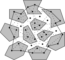
Figure 7. The sets $S_{i}$ and the convex hull $\operatorname{conv}_{C}(S)$ with respect to cone $C$. The $\mathcal{D}$-Delaunay triangulation is drawn dotted.

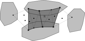
Figure 8. The corridor $R$ which is split into two sub-corridors and two tri-colored triangles. The corners of the sub-corridors are marked by crosses.

Let $G$ be the $\mathcal{D}$-Delaunay graph of the set of colored points $\bar{S}$, i.e. $G=\operatorname{DT}(\bar{S})$. $G$ is indeed a triangulation (cf. lemma 1.8). In this graph we call a triangle uni-colored, bi-colored or tri-colored depending upon the number of colors its vertices have. In a similar way we call edges uni-colored or bi-colored. We call a maximal connected chain of bi-colored triangles in $G$ sharing bi-colored edges a corridor (cf. figure 8). Since the graph $G$ is planar and each of the induced subgraphs $G\cap D_{i}$ is connected according to lemma 1.10 the number of such corridors is at most $3k-6$ ([14]). All colorless points are contained in the corridors and the tri-colored triangles because any uni-colored triangle is contained it its color-defining object. We break each corridor $R$ into a minimum number of sub-corridors, i.e. sub-chains of the chain that forms $R$, so that each sub-corridor contains at most $\delta n$ colorless points. Since there are less than $n$ colorless points and since the total number of corridors is $3k-6$ the total number of sub-corridors is $O(1/\delta)$.

Each sub-corridor is bounded by two chains of uni-colored edges which we call sides and by two bi-colored edges which we call ends of the sub-corridor. The endpoints of the sides are called corners. Let $N\subseteq S$ be the set of all corners of all sub-corridors. Since each sub-corridor has at most 4 corners the size of $N$ is $O(1/\epsilon)$. The set $N$ is an epsilon-net for the set of non-piercing objects $\mathcal{D}$.

The proof that $N$ is indeed an epsilon-net relies in principle on the fact that the collection $\mathcal{D}$ are non-piercing objects and follows along the lines of [14].

Proof 1.16.

Let $D$ be an object that has no points of $S$ on its boundary (cf. lemma 1.12) and assume that $D$ does not contain any points from $N$. The theorem is proven when we can show that $D$ then contains less than $\epsilon n$ points of $S$. If $D$ contains no colored point then we are done, because the sets $S_{i}$ were a maximal. Hence, $D$ must contain at least one colored point. If it contains two colored points, lets say $z_{1}$ of color 1 and $z_{2}$ of color 2, we can draw the following picture: Let $D_{1}$ be the color defining object of color 1 and $D_{2}$ the color defining object of color $2$. Then $D$ intersects $D_{1}$ and $D_{2}$ but cannot pierce them. The area between $D_{1}$ and $D_{2}$ is a sub-corridor whose ends we denote by $(a_{1},a_{2})$ and $(b_{1},b_{2})$. Lemma 1.14 assures that there is an object $D_{a}$ that has $a_{1}$ and $a_{2}$ on its boundary and there is an object $D_{b}$ that has $b_{1}$ and $b_{2}$ on its boundary. Since $D$ also does not contain any point from $N$ which are the corners of the sub-corridors, i.e. it does not contain $a_{1},a_{2},b_{1}$ or $b_{2}$ and since $D$ and $D_{a}$ as well as $D$ and $D_{b}$ are non-piercing it must lie between two ends of one sub-corridor. See figure 10 for an illustration. Now, as all objects $D_{1}$, $D_{2}$, $D_{a}$ and $D_{b}$ contain at most $\delta n$ points and the sub-corridor also contains at most $\delta n$ points $D$ can contain at most $5\cdot\delta n=5/6\epsilon n<\epsilon n$ points of $S$.

Figure 9. The case where $D$ contains colored points of at least two colors.

Figure 10. The case where $D$ contains colored points of exactly one color.

The case where $D$ only contains points of one color and colorless points is very similar. There is basically only one setup and it is depicted in figure 10. Arguing as above it easy to see in this case that $D$ cannot contain more than $4\cdot\delta n<\epsilon n$ points from $S$.

Hence, we have the following theorem

Theorem 1.17.

Let $\mathcal{D}$ be the set of non-piercing objects in $\mathbb{R}^{2}$, that is produced by the projection $\tau$. For every finite point set in non-$\mathcal{D}$-degenerate position there exists an epsilon-net of size $O(1/\epsilon)$.

Together with lemma 1.1 and lemma 1.3 this immediately implies our main theorem

Theorem 1.18.

Given a finite point set $P\subseteq\mathbb{R}^{3}$ and a polytope $T\subseteq\mathbb{R}^{3}$. The set system $(P,\mathcal{T})$ induced by a set of translates of polytope $T$ admits an epsilon-net of size $O(1/\epsilon)$.

2. From Epsilon-Nets to Hitting Sets

In this section we will describe a constant factor approximation algorithm to the hitting set problem using the epsilon-net of size $O(1/\epsilon)$ from the previous section. Recall that in the hitting set problem we are given a set of points $P\in\mathbb{R}^{3}$ and a set polytopes that are all translates of the same polytope and we would like to select a subset $H\subseteq P$ of the input points of minimal cardinality such that every polytope is stabbed by a point in $H$. We denote the corresponding set system by $(P,\mathcal{T})$. The fractional hitting set problem is a relaxation of the original hitting set problem and is defined by the following linear program:

$$\min \sum_{p\in P}x(p)$$ (1)

$$\operatorname{s.t.} \forall T\in\mathcal{T} \sum_{p\in T}x(p)\geq 1$$ (2)

$$\forall p\in P x(p)\geq 0$$ (3)

Let $\operatorname{OPT}$ denote the optimal size of the hitting set and $\operatorname{OPT}^{*}$ the optimal value of the fractional hitting set problem. It is known that the integrality gap is constant for set systems that admit an epsilon-net of size $O(1/\epsilon)$ [15].

Let $w:P\to\mathbb{R}_{\geq 0}$ be a weight function for the set $P$. We define the weight $w(A)$ of a subset $A\subseteq P$ to be the sum of the weights of the elements of $A$. The weighted version of an epsilon-net is as follows: Consider a set system $(P,\mathcal{T})$ and a weight function $w:P\to\mathbb{R}_{\geq 0}$. A set $H\subseteq P$ is called an epsilon-net with respect to $w$ if $H\cap R\neq\emptyset$ for every subset $T\in\mathcal{T}$ for which $w(T)\geq\epsilon\cdot w(S)$. There are algorithms that compute a hitting set provided one has an epsilon-net finder. The core idea to all these algorithms is to find a weight function $w:P\to\mathbb{R}_{\geq 0}$ that assigns weights to the elements of $P$ and finds an appropriate $\epsilon$ such that every set in $\mathcal{T}$ has weight at least $\epsilon\cdot w(S)$. Once such weights are found it is then obvious that an epsilon-net to this set system is automatically a hitting set.

The algorithm given by Brönnimann and Godrich [3] computes these weights iteratively. Initially, all elements have weight $1$. Then, in each iteration an epsilon-net is computed and then checked whether it is also a proper hitting set. If not, i.e. there is a set which is not hit, then the weights of its elements are doubled. This is done until a hitting set is found. This algorithm can be seen as a deterministic analogue of the randomized natural selection technique used for instance by Clarkson [4].

Another algorithm is by Even et al. [7]. Here, the weights of the elements and $\epsilon$ are directly found by the following linear program:

$$\max\epsilon$$ (4)

$$\operatorname{s.t.} \forall T\in\mathcal{T} w(T)\geq\epsilon$$ (6)

$$\sum_{p\in P}w(p)=1$$

$$\forall p\in P w(p)\geq 0$$ (7)

It suffices to approximate the solution to this linear problem. There are numerous algorithms that find an approximate solution to such a covering linear program efficiently [18, 8].

One can reduce the problem of finding a weighted epsilon-net to the unweighted case. One just makes multiple copies of a point according to its assigned weight and it can be shown that the cardinality of this multiset can be bounded by $2n$ [5]. Hence, an $\frac{\epsilon}{2}$-net for this set system gives a hitting set for the original hitting set problem. Hence, we have

Theorem 2.1.

There exists a polynomial time algorithm that computes a constant-factor approximation to the hitting set problem for translates of polytopes in $\mathbb{R}^{3}$.

3. From Hitting Set to Set Cover

The dual set system of a set system $(P,\mathcal{T})$ is the set system $(\mathcal{T},P^{*})$ where $P^{*}=\{\mathcal{T}_{p}:p\in P\}$ and $\mathcal{T}_{p}$ consists of all subsets of $\mathcal{T}$ that contain $p$.

Obviously, a set cover for the primal set system is a hitting set for the dual set system. Hence, in order to solve the set cover problem for a set system it suffices to solve the hitting set problem for the dual set system. For arbitrary set systems, the dual set system can be of quite different structure. In general it is only known that the VC-dimension of the dual set system is less than $2^{d+1}$, where $d$ is the VC-dimension of the primal set system [1].

However, we observe that if the set system is induced by translates of a polytope, then the dual is again induced by translates of a polytope. To see this, let $(P,\mathcal{T})$ be the primal set system. One just reduces each polytope $T\in\mathcal{T}$ to a point, for instance each to its lowest vertex. Let this be the set $P^{\prime}$. Then, replace each point of $P$ by a translate of the polytope $T^{\prime}$ which is the inversion of $T$ in a point. One easily verifies that the so constructed set system $(P^{\prime},\mathcal{T}^{\prime})$ of points $P^{\prime}$ and collection of translates of polytope $T^{\prime}$ is indeed equivalent to the dual $(\mathcal{T},P^{*})$. This holds in fact for all $\mathbb{R}^{d}$. Hence, we can find a constant-factor approximation to the set cover problem for translates of a polytope in $\mathbb{R}^{3}$ in polynomial time. This brings us to our final theorem

Theorem 3.1.

There exists a polynomial time algorithm that computes a constant-factor approximation to the set cover problem for translates of polytopes in $\mathbb{R}^{3}$.

4. Conclusions and Open Problems

In this paper we have given the first constant-factor approximation algorithm for finding a set cover for a set of points in $\mathbb{R}^{3}$ by a given collection of translates of a polytope as well as the first constant-factor approximation algorithm for the corresponding hitting set problem. We achieved this result by providing an epsilon-net of size $O(\frac{1}{\epsilon})$ for the corresponding set system which is optimal up to a multiplicative constant. Eventhough we can approximate a unit ball in $\mathbb{R}^{3}$ up to any given precision by a polytope, the corresponding question, whether there exists a constant-factor approximation algorithm for unit balls in $\mathbb{R}^{3}$ still remains open.

References

- [1] P. Assouad. Densité et dimension. Ann. Inst. Fourier, 33(3):233–282, 1983.
- [2] A. Blumer, A. Ehrenfeucht, D. Haussler, and M. K. Warmuth. Learnability and the vapnik-chervonenkis dimension. J. ACM, 36(4):929–965, 1989.
- [3] H. Brönnimann and M. T. Goodrich. Almost optimal set covers in finite vc-dimension: (preliminary version). In SoCG ’94, pages 293–302, New York, NY, USA, 1994. ACM Press.
- [4] K. Clarkson. Las vegas algorithms for linear and integer programming when the dimension is small. J. ACM, 42(2):488–499, 1995.
- [5] K. L. Clarkson and K. Varadarajan. Improved approximation algorithms for geometric set cover. In SoCG ’05, pages 135–141, New York, NY, USA, 2005. ACM Press.
- [6] H. Edelsbrunner and E. Welzl. On the number of line separations of a finite set in the plane. J. Comb. Theory, Ser. A, 38(1):15–29, 1985.
- [7] G. Even, D. Rawitz, and S. Shahar. Hitting sets when the vc-dimension is small. Inf. Process. Lett., 95(2):358–362, 2005.
- [8] N. Garg and J. Könemann. Faster and simpler algorithms for multicommodity flow and other fractional packing problems. In FOCS ’98, page 300, Washington, DC, USA, 1998. IEEE Computer Society.
- [9] D. S. Hochbaum and W. Maass. Approximation schemes for covering and packing problems in image processing and vlsi. J. ACM, 32(1):130–136, 1985.
- [10] J. Komlós, J. Pach, and G. J. Woeginger. Almost tight bounds for epsilon-nets. Discrete and Computational Geometry, 7:163–173, 1992.
- [11] C. Lund and M. Yannakakis. On the hardness of approximating minimization problems. J. ACM, 41(5):960–981, 1994.
- [12] J. Matousek. Lectures on Discrete Geometry. Springer-Verlag New York, Inc., Secaucus, NJ, USA, 2002.
- [13] J. Matoušek. Reporting points in halfspaces. Comput. Geom. Theory Appl., 2(3):169–186, 1992.
- [14] J. Matoušek, R. Seidel, and E. Welzl. How to net a lot with little: Small epsilon-nets for disks and halfspaces. In SoCG ’90, pages 16–22, 1990.
- [15] J. Pach and P. K. Agarwal. Combinatorial Geometry. Wiley, New York, 1995.
- [16] J. Pach and G. Woeginger. Some new bounds for epsilon-nets. In SoCG ’90, pages 10–15, New York, USA, 1990. ACM Press.
- [17] V. N. Vapnik and A. Ya. Chervonenkis. On the uniform convergence of relative frequencies of events to their probability. Theory Probab. Appl., 16:264–280, 1971.
- [18] N. E. Young. Randomized rounding without solving the linear program. In SODA ’95, pages 170–178, Philadelphia, PA, USA, 1995. Society for Industrial and Applied Mathematics.