Computing Minimum Spanning Trees with Uncertainty

Abstract.

We consider the minimum spanning tree problem in a setting where information about the edge weights of the given graph is uncertain. Initially, for each edge $e$ of the graph only a set $A_{e}$, called an uncertainty area, that contains the actual edge weight $w_{e}$ is known. The algorithm can ‘update’ $e$ to obtain the edge weight $w_{e}\in A_{e}$. The task is to output the edge set of a minimum spanning tree after a minimum number of updates. An algorithm is $k$-update competitive if it makes at most $k$ times as many updates as the optimum. We present a $2$-update competitive algorithm if all areas $A_{e}$ are open or trivial, which is the best possible among deterministic algorithms. The condition on the areas $A_{e}$ is to exclude degenerate inputs for which no constant update competitive algorithm can exist.

Next, we consider a setting where the vertices of the graph correspond to points in Euclidean space and the weight of an edge is equal to the distance of its endpoints. The location of each point is initially given as an uncertainty area, and an update reveals the exact location of the point. We give a general relation between the edge uncertainty and the vertex uncertainty versions of a problem and use it to derive a $4$-update competitive algorithm for the minimum spanning tree problem in the vertex uncertainty model. Again, we show that this is best possible among deterministic algorithms.

2008277-288Bordeaux 277

1. Introduction

In many applications one has to deal with computational problems where some parts of the input data are imprecise or uncertain. For example, in a geometric problem involving sets of points, the locations of the points might be known only approximately; effectively this means that instead of the location of a point, only a region or area containing that point is known. In other applications, only estimates of certain input parameters may be known, for example in form of a probability distribution. There are many different approaches to dealing with problems of this type, including e.g. stochastic optimization and robust optimization.

Pursuing a different approach, we consider a setting in which the algorithm can obtain exact information about an input data item using an update operation, and we are interested in the update complexity of an algorithm, i.e., our goal is to compute a correct solution using a minimum number of updates. The updates are adaptive, i.e., one selects the next item to update based on the result of the updates performed so far, so we refer to the algorithm as an on-line algorithm. There are a number of application areas where this setting is meaningful. For example, in a mobile ad-hoc network an algorithm may have knowledge about the approximate locations of all nodes, and it is possible (but expensive) to find out the exact current location of a node by communicating to that node and requesting that information. To assess the performance of an algorithm, we compare the number of updates that the algorithm makes to the optimal number of updates. Here, optimality is defined in terms of an adversary, who, knowing the values of all input parameters, makes the fewest updates needed to present a solution to the problem that is provably correct, in that no additional areas need to be updated to verify the correctness of the solution claimed by the adversary. We say that an algorithm is $k$-update competitive if, for each input instance, the algorithm makes at most $k$ times as many updates as the optimum number of updates for that input instance. The notions of update complexity and $k$-update competitive algorithms were implicit in Kahan’s model for data in motion [6] and studied further for two-dimensional geometric problems by Bruce et al. [2].

In this paper, we consider the classical minimum spanning tree (MST) problem in two settings with uncertain information. In the first setting, the edge weights are initially given as uncertainty areas, and the algorithm can obtain the exact weight of an edge by updating the edge. If the uncertainty areas are trivial (i.e., contain a single number) or (topologically) open, we give a $2$-update competitive algorithm and show that this is best possible for deterministic algorithms. Without this restriction on the areas, it is easy to construct degenerate inputs for which there is no constant update competitive algorithm. Although degeneracy could also be excluded by other means (similar to the “general position” assumption in computational geometry), our condition is much cleaner.

In the second setting that we consider, the vertices of the graph correspond to points in Euclidean space, and the locations of the points are initially given as uncertainty areas. The weight of an edge equals the distance between the points corresponding to its vertices. The algorithm can update a vertex to reveal its exact location. We give a general relation between the edge uncertainty version and the vertex uncertainty version of a problem. For trivial or open uncertainty areas we obtain a $4$-update competitive algorithm for the MST problem with vertex uncertainty and show again that this is optimal for deterministic algorithms.

Related Work.  We do not attempt to survey the vast literature dealing with problems on uncertain data, but focus on work most closely related to ours. Kahan [6] studied the problem of finding the maximum, the median and the minimum gap of a set of $n$ real values constrained to fall in a given set of $n$ real intervals. In the spirit of competitive analysis, he defined the lucky ratio of an update strategy as the worst-case ratio between the number of updates made by the strategy and the optimal number of updates of a non-deterministic strategy. In our terminology, a strategy with lucky ratio $k$ is $k$-update competitive. Kahan gave strategies with optimal lucky ratios for the problems considered [6].

Bruce et al. studied the problems of computing maximal points or the points on the convex hull of a set of uncertain points [2] and presented $3$-update competitive algorithms. They introduced a general method, called the witness algorithm, for dealing with problems involving uncertain data, and derived their $3$-update competitive algorithms using that method. The algorithms we present in this paper are based on the method of the witness algorithm of [2], but the application to the MST problem is non-trivial.

Feder et al. [5, 4], consider two problems in a similar framework to ours. Firstly, they consider the problem of computing the median of $n$ numbers to within a given tolerance. Each input number lies in an interval, and an update reveals the exact value, but different intervals have different update costs. They consider off-line algorithms, which must decide the sequence of updates prior to seeing the answers, as well as on-line ones, aiming to minimize the total update cost. In [4], off-line algorithms for computing the length of a shortest path from a source $s$ to a given vertex $t$ are considered. Again, the edge lengths lie in intervals with different update costs, and they study the computational complexity of minimizing the total update cost.

One difference between the framework of Feder et al. and ours is that they require the computation of a specific numeric value (the value of the median, the length of a shortest path). We, on the other hand, aim to obtain a subset of edges that form an MST. In general, our version of the problem may require far fewer updates. Indeed, for the MST with vertex uncertainties, it is obvious that one must update all non-trivial areas to compute the cost of the MST exactly. However, the cost of the MST may not be needed in many cases: if the MST is to be used as a routing structure in a wireless ad-hoc network, then it suffices to determine the edge set. Also, our algorithms aim towards on-line optimality against an adversary, whereas their off-line algorithms aim for static optimality.

Further work in this vein attempts to compute other aggregate functions to a given degree of tolerance, and establishes tradeoffs between update costs and error tolerance or presents complexity results for computing optimal strategies, see e.g. [10, 8].

Another line of work considers the robust spanning tree problem with interval data. For a given graph with weight intervals specified for its edges, the goal is to compute a spanning tree that minimizes the worst-case deviation from the minimum spanning tree (also called the regret), over all realizations of the edge weights. This is an off-line problem, and no update operations are involved. The problem is proved $\mathcal{NP}$-hard in [1]. A $2$-approximation algorithm is given in [7]. Further work has considered heuristics or exact algorithms for the problem, see e.g. [12].

In the setting of geometric problems with imprecise points, Löffler and van Kreveld have studied the problem of computing the largest or smallest convex hull over all possible locations of the points inside their uncertainty areas [9]. Here, the option of updating a point does not exist, and the goal is to design fast algorithms computing an extremal solution over all possible choices of exact values of the input data.

The remainder of the paper is organized as follows. In Section 2, we define our problems and introduce the witness algorithm of [2] in general form. Sections 3 and 4 give our results for MSTs with edge and vertex uncertainty, respectively.

2. Preliminaries

The mst-edge-uncertainty problem is defined as follows: Let $G=(V,E)$ be a connected, undirected, weighted graph. Initially the edge weights $w_{e}$ are unknown; instead, for each edge $e$ an area $A_{e}$ is given with $w_{e}\in A_{e}$. When updating an edge $e$, the value of $w_{e}$ is revealed. The aim is to find (the edge set of) an MST for $G$ with the least number of updates.

In applications such as mobile ad-hoc networks it is natural to assume the vertices of our graph are embedded in two or three dimensional space. This leads to the mst-vertex-uncertainty problem defined as follows: Let $G=(V,E)$ be a connected, undirected, weighted graph. The vertices correspond to points in Euclidean space. We refer to the point $p_{v}$ corresponding to a vertex $v$ as its location. The weight of an edge is the Euclidean distance between the locations of its vertices. Initially the locations of the vertices are not known; instead, for each vertex $v$ an area $A_{v}$ is given with $p_{v}\in A_{v}$, where $p_{v}$ is the actual location of vertex $v$. When a vertex $v$ is updated, the location $p_{v}$ is revealed. The aim is to find an MST for $G$ with the least number of updates.

Formally we are interested in on-line update problems of the following type: Each problem instance $P=(C,A,\phi)$ consists of an ordered set of data $C=\{c_{1},\dots,c_{n}\}$, also called a configuration, and a function $\phi$ such that $\phi(C)$ is the set of solutions for $P$. (The function $\phi$ is the same for all instances of a problem and can thus be taken to represent the problem.) At the beginning the set $C$ is not known to the algorithm; instead, an ordered set of areas $A=\{A_{1},\dots,A_{n}\}$ is given, such that $c_{i}\in C$ is an element of $A_{i}$. The sets $A_{i}$ are called areas of uncertainty or uncertainty areas for $C$. We say that an uncertainty area $A_{i}$ that consists of a single element is trivial. For example, in the mst-edge-uncertainty problem, $C$ consists of the given graph $G=(V,E)$ and its $|E|$ actual edge weights. The ordered set of areas $A$ specifies the graph $G$ exactly (so we assume complete knowledge of $G$) and, for each edge $e\in E$, contains an area $A_{e}$ giving the possible values the weight of $e$ may take. Then $\phi(C)$ is the set of MSTs of the graph with edge weights given by $C$, each tree represented as a set of edges.

For a given set of uncertainty areas $A=\{A_{1},\dots,A_{n}\}$, an area $A_{i}$ can be updated, which reveals the exact value of $c_{i}$. After updating $A_{i}$, the new ordered set of areas of uncertainty for $C$ is $\{A_{1},\dots,A_{i-1},\{c_{i}\},A_{i+1},\dots,A_{n}\}$. Updating all non-trivial areas would reveal the configuration $C$ and would obviously allow us to calculate an element of $\phi(C)$ (under the natural assumption that $\phi$ is computable). The aim of the on-line algorithm is to minimize the number of updates needed in order to compute an element of $\phi(C)$.

An algorithm is $k$-update competitive for a given problem $\phi$ if for every problem instance $P=(C,A,\phi)$ the algorithm needs at most $k\cdot\mathit{OPT}+c$ updates, where $c$ is a constant and $\mathit{OPT}$ is the minimum number of updates needed to verify an element of $\phi(C)$. (For our algorithms we can take $c=0$, but our lower bounds apply also to the case where $c$ can be an arbitrary constant.) Note that the primary aim is to minimize the number of updates needed to calculate a solution. We do not consider running time or space requirements in detail, but note that our algorithms are clearly polynomial, provided that one can obtain the infimum and supremum of an area in $O(1)$ time, an assumption which holds e.g. if areas are open intervals.

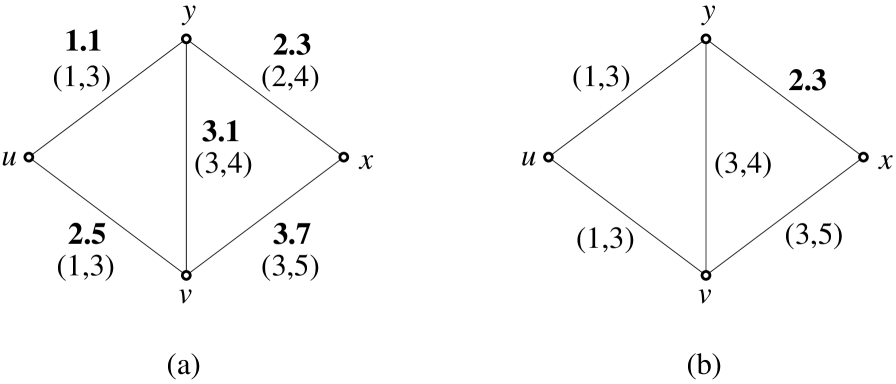
Figure 1. (a) Instance of mst-edge-uncertainty   (b) Updating the edge $\{x,y\}$ suffices to verify an MST

As an example, consider the instance of mst-edge-uncertainty shown in Figure 1(a), where each edge is labeled with its actual weight (in bold) and its uncertainty area (an open interval). Updating the edge $\{x,y\}$ leads to the situation shown in Figure 1(b) and suffices to verify that the edges $\{u,y\}$, $\{u,v\}$ and $\{x,y\}$ form an MST regardless of the exact weights of the edges that have not yet been updated. If no edge is updated, one cannot exclude that an MST includes the edge $\{v,x\}$ instead of $\{x,y\}$, as the former could have weight $3.3$ and the latter weight $3.9$, for example. Therefore, for the instance of mst-edge-uncertainty in Figure 1(a) the minimum number of updates is $1$.

2.1. The Witness Algorithm

The witness algorithm for problems with uncertain input was first introduced in [2]. This section describes the witness algorithm in a more general setting and notes some of its properties. We call $W\subseteq A$ a witness set of $(A,\phi)$ if for every possible configuration $C$ (where $c_{i}\in A_{i}$) no element of $\phi(C)$ can be verified without updating an element of $W$. In other words, any set of updates that suffices to verify a solution must update at least one area of $W$. The witness algorithm for a problem instance $P=(C,A,\phi)$ is shown in Figure 2.

if an element of $\phi(C)$ can not be calculated from $A$ then

find a witness set $W$

update all areas in $W$

let $A^{\prime}$ be the areas of uncertainty after updating $W$

restart the algorithm with $P^{\prime}=(C,A^{\prime},\phi)$

end if

return an element of $\phi(C)$ that can be calculated from $A$

Figure 2. The general witness algorithm

For two ordered sets of areas $A=\{A_{1},A_{2},\dots,A_{n}\}$ and $B=\{B_{1},B_{2},\dots,B_{n}\}$ we say that $B$ is at least as narrow as $A$ if $B_{i}\subseteq A_{i}$ for all $1\leq i\leq n$. The following lemma is easy to prove.

Lemma 2.1.

Let $P=(C,A,\phi)$ be a problem instance and $B$ be a narrower set of areas than $A$. Further let $W$ be a witness set of $(B,\phi)$. Then $W$ is also a witness set of $(A,\phi)$.

Theorem 2.2.

If there is a global bound $k$ on the size of any witness set used by the witness algorithm, then the witness algorithm is $k$-update competitive.

Theorem 2.2 was proved in a slightly different setting in [2], but the proof carries over to the present setting in a straightforward way by using Lemma 2.1.

3. Minimum Spanning Trees with Edge Uncertainty

In this section we present an algorithm u-red for the problem mst-edge-uncertainty. In the case that all areas of uncertainty are either open or trivial, algorithm u-red is $2$-update competitive, which we show is optimal. Furthermore, we show that for arbitrary areas of uncertainty there is no constant update competitive algorithm.

First, let us recall a well known property, usually referred to as the red rule [11], of MSTs:

Proposition 3.1.

Let $G$ be a weighted graph and let $C$ be a cycle in $G$. If there exists an edge $e\in C$ with $w_{e}>w_{e^{\prime}}$ for all $e^{\prime}\in C-\{e\}$, then $e$ is not in any MST of $G$.

We will use the following notations and definitions: A graph $\mathcal{U}=(V,E)$ with an area $A_{e}$ for each edge $e\in E$ is called an edge-uncertainty graph. We say a weighted graph $G=(V,E)$ with edge weights $w_{e}$ is a realization of $\mathcal{U}$ if $w_{e}\in A_{e}$ for every $e\in E$. Note that $w_{e}$ is associated with $G$ and $A_{e}$ with $\mathcal{U}$. We also say that an edge $e$ is trivial if the area $A_{e}$ is trivial.

For an edge $e$ in an edge-uncertainty graph we denote the upper limit of $A_{e}$ by $U_{e}=\sup A_{e}$ and the lower limit of $A_{e}$ by $L_{e}=\inf A_{e}$.

We extend the notion of an MST to edge-uncertainty graphs in the following way: Let $\mathcal{U}$ be an edge-uncertainty graph. We say $T$ is an MST of $\mathcal{U}$ if $T$ is an MST of every realization of $\mathcal{U}$. Clearly not every edge-uncertainty graph has an MST.

Let $C$ be a cycle in $\mathcal{U}$. We say the edge $e\in C$ is an always maximal edge in $C$ if $L_{e}\geq U_{c}$ for all $c\in C-\{e\}$. Therefore in every realization $G$ of $\mathcal{U}$ we have $w_{e}\geq w_{c}$ for all $c\in C-\{e\}$.

Note that a cycle can have more than one always maximal edge and not every cycle has an always maximal edge. The following lemma deals with cycles of the latter kind:

Lemma 3.2.

Let $\mathcal{U}$ be an edge-uncertainty graph. Let $C$ be a cycle in $\mathcal{U}$. Let $C$ not have an always maximal edge. Then for any $f\in C$ with $U_{f}=\max\{U_{c}\mid c\in C\}$ we have that $f$ is non-trivial and there exists an edge $g\in C-\{f\}$ with $U_{g}>L_{f}$.

Proof 3.3.

Let $f\in C$ be an edge with $U_{f}=\max\{U_{c}\mid c\in C\}$. If $L_{f}=U_{f}$ the edge $f$ would be always maximal. Hence $L_{f}$ must be strictly smaller than $U_{f}$ and $f$ is non-trivial. Since there is no always maximal edge in $C$, we have that $L_{f}<\max\{U_{c}\mid c\in C-\{f\}\}$. Therefore there exists at least one edge $g$ in $C-\{f\}$ with $L_{f}<U_{g}$.

Proposition 3.4.

Let $\mathcal{U}$ be an edge-uncertainty graph with an MST $T$. Let $f=\{u,v\}$ be an edge of $\mathcal{U}$ such that $f\not\in T$. Let $P$ be the path in $T$ connecting $u$ and $v$, then $U_{p}\leq L_{f}$ for all $p\in P$.

Proof 3.5.

Assume there exists a $p\in P$ with $U_{p}>L_{f}$. Then there exists a realization $G$ of $\mathcal{U}$ with $w_{p}>w_{f}$. Hence by removing the edge $p$ and adding the edge $f$ to $T$ we obtain a spanning tree that is cheaper than $T$. So $T$ is not an MST for $G$. This is a contradiction since $T$ is an MST of $\mathcal{U}$ and therefore of any realization of $\mathcal{U}$.

Our algorithm u-red applies the red rule to the given uncertainty graph, but we have to be careful about the order in which edges are considered. The order we use is as follows: Let $\mathcal{U}$ be an edge-uncertainty graph and let $e,f$ be two edges in $\mathcal{U}$. We say

• $e<f$ if $L_{e}<L_{f}$ or ($L_{e}=L_{f}$ and $U_{e}<U_{f}$),

• $e\leq f$ if $e<f$ or ($L_{e}=L_{f}$ and $U_{e}=U_{f}$).

Edges with the same upper and lower weight limit are ordered arbitrarily.

01 Index all edges such that $e_{1}\leq e_{2}\leq\dots\leq e_{m}$.

02 Let $\Gamma$ be $\mathcal{U}$ without any edge

03 for $i$ from $1$ to $m$ do
04           add $e_{i}$ to $\Gamma$

05           if $\Gamma$ has a cycle $C$ then
06                  if $C$ contains an always maximal edge $e$ then
07                           delete $e$ from $\Gamma$

08                  else

09                           let $f\in C$ such that $U_{f}=\max\{U_{c}|c\in C\}$

10                           let $g\in C-\{f\}$ such that $U_{g}>L_{f}$

11                           update $f$ and $g$

12                           restart the algorithm

13                  end if

14          end if
15 end for

16 return $\Gamma$

Figure 3. Algorithm u-red

Algorithm u-red is shown in Figure 3. Observe that:

• In case no update is made the algorithm u-red will perform essentially Kruskal’s algorithm [3]. When a cycle is created there will be an always maximal edge in that cycle. Due to the order in which the algorithm adds the edges to $\Gamma$ the edge $e_{i}$ that closes a cycle $C$ must be an always maximal edge in $C$. So where Kruskal’s algorithm does not add an edge to $\Gamma$ when it would close a cycle, the u-red algorithm adds this edge to $\Gamma$ but then deletes it or an equally weighted edge in the cycle from $\Gamma$.

• By Lemma 3.2 the edges $f,g$ in line $9$ and $10$ exist and $f$ is non-trivial.

• The algorithm will terminate. The algorithm either updates at least one non-trivial edge $f$ and restarts, or does not perform any updates. Hence the algorithm u-red will eventually return an MST of $G$.

• During the run of the algorithm the graph $\Gamma$ is either a forest or contains one cycle. In case the most recently added edge closes a cycle either one edge of the cycle will be deleted or after some updates the algorithm restarts and $\Gamma$ has no edges. Hence at any given time there is at most one cycle in $\Gamma$.

As the algorithm may restart itself, we say a run is completed if the algorithm restarts or returns the MST. In case of a restart, another run of the algorithm starts.

Before showing that the algorithm u-red is $2$-update competitive under the restriction to open or trivial areas, we discuss some technical preliminaries. In each run the algorithm considers all edges in a certain order $e_{1},\dots,e_{m}$. During the run of the algorithm we refer to the currently considered edge as $e_{i}$. Let $u$ and $v$ be two distinct vertices. In case $u$ and $v$ are in the same connected component of the subgraph with edges $e_{1},\ldots,e_{i-1}$, then they are also connected in the current $\Gamma$. Furthermore, we need some properties of a path connecting $u$ and $v$ in $\Gamma$ under certain conditions. The next two lemmas establish these properties. They are technical and are solely needed in the proof of Lemma 3.9.

Lemma 3.6.

Let $h=\{u,v\}$ and $e$ be two edges in $\mathcal{U}$. Let $h\neq e$ and $L_{h}<U_{e}$. Let the algorithm be in a state such that $h$ has been considered. Then $u$ and $v$ are connected in the current $\Gamma-\{e\}$.

Proof 3.7.

If the edge $h$ is in the current $\Gamma$ then clearly $u$ and $v$ are connected in $\Gamma-\{e\}$, so assume that $h$ is no longer in $\Gamma$. Therefore it must have been an always maximal edge in a cycle $C$. In order for $h$ to be an always maximal edge in $C$ we must have that $L_{c}\leq U_{c}\leq L_{h}$ for all $c\in C-\{h\}$. So since $L_{h}<U_{e}$ we have that $L_{c}<U_{e}$. Also the edge $h$ can not be an always maximal edge in $C$ if $C$ contains $e$.

Clearly $C-\{h\}$ is a path in $U$ connecting $u$ and $v$ and does not contain $e$. Since the edges in $C-\{h\}$ might have been deleted from the current $\Gamma$ themselves we have to use this argument repeatedly, but eventually we get a path in the current $\Gamma-\{e\}$ connecting $u$ and $v$.

The next lemma follows directly from Lemma 3.6.

Lemma 3.8.

Let $u,v$ be vertices and $e$ be an edge in $\mathcal{U}$. Let $P$ be a path in $\mathcal{U}-\{e\}$ connecting $u$ and $v$ with $L_{p}<U_{e}$ for all $p\in P$. Let the algorithm be in a state such that all edges of $P$ have been considered, then there exists a path $P^{\prime}$ in the current $\Gamma$ connecting $u$ and $v$ with $e\not\in P^{\prime}$.

Lemma 3.9.

Assume that all uncertainty areas are open or trivial. The edges $f$ and $g$ as described in the algorithm u-red at line $9$ and $10$ form a witness set.

Proof 3.10.

We have the following situation: There exist a cycle $C$ in $\Gamma$ with no always maximal edge. Let $m=\max\{U_{c}~{}|~{}c\in C\}$. The edges $f$ and $g$ are in $C$ with $U_{f}=m$ and $U_{g}>L_{f}$. By Lemma 3.2 the area $A_{f}$ is non-trivial.

We now assume that the set $\{f,g\}$ is not a witness set. So we can update some edges, but not $f$ or $g$ such that the resulting edge-uncertainty graph $\mathcal{U}^{\prime}$ has an MST $T$. Let $U^{\prime}_{e}$ and $L^{\prime}_{e}$ denote the upper and lower limit of an area for an edge $e$ with regard to $\mathcal{U}^{\prime}$. Since both edges $f$ and $g$ are not updated we note that

$$L_{f}=L^{\prime}_{f},U_{f}=U^{\prime}_{f},L_{g}=L^{\prime}_{g},U_{g}=U^{\prime}_{g}.$$

Since all areas in $\mathcal{U}^{\prime}$ and $\mathcal{U}$ are either trivial or open, and $C$ has no always maximal edge, the weight of every edge in $C$ must be less than $m$. In particular we have that for all $c\in C$

$$U^{\prime}_{c}<m\mbox{ or }L^{\prime}_{c}<U_{c}=m.$$

Since $U_{f}=m$ there exists a realization $G^{\prime}$ of $\mathcal{U}^{\prime}$ and $\mathcal{U}$, where the weight of $f$ is greater than the weight of any other edge in $C$. By Proposition 3.1 the edge $f$ is not in any MST of $G^{\prime}$ and therefore also not in $T$.

Let $u$ and $v$ be the vertices of $f$. By Proposition 3.4 there exists a path $P$ in $\mathcal{U}^{\prime}$ connecting $u$ and $v$ with $U^{\prime}_{p}\leq L_{f}$ for all $p\in P$. Since $U_{g}>L_{f}$ and neither $f$ nor $g$ are updated the edge $g$ is not in the path $P$. We now argue that all edges of $P$ must have been already considered by the algorithm. For this we look at the following two cases:

Case 1) Let $p\in P$ and $L^{\prime}_{p}<L_{f}$. Since $L_{p}\leq L^{\prime}_{p}$ we have that $L_{p}<L_{f}$.

Case 2) Let $p\in P$ and $L^{\prime}_{p}=L_{f}$. Since $U^{\prime}_{p}\leq L_{f}$ we have that $L^{\prime}_{p}=U^{\prime}_{p}=L_{f}$. Either the area $A_{p}$ is also trivial ($L_{p}=U_{p}=L^{\prime}_{p}=U^{\prime}_{p}=L_{f}$) or $A_{p}$ is open and contains the point $L^{\prime}_{p}$, in this case $L_{p}<L^{\prime}_{p}$.

So for all $p\in P$ we have $L_{p}<L_{f}\mbox{ or }L_{p}=U_{p}=L_{f}<U_{f}$. Therefore all edges of $P$ will be considered before $f$. We also note that $L_{p}\leq L^{\prime}_{p}\leq L_{f}<U_{g}$ for all $p\in P$. By Lemma 3.8 there exists a path $P^{\prime}$ in $\Gamma$ connecting $u$ and $v$ and $g\not\in P^{\prime}$. Hence $\Gamma$ has two cycles, which is a contradiction.

Using Theorem 2.2, this leads directly to the following result.

Theorem 3.11.

Under the restriction to open and trivial areas the algorithm u-red is $2$-update competitive.

We remark that the analysis of algorithm u-red actually works also in the more general setting where it is only required that every area is trivial or satisfies the following condition: the area contains neither its infimum nor its supremum. It remains to show that under the restriction to open and trivial areas there is no algorithm for the mst-edge-uncertainty problem that is $(2-\epsilon)$-update competitive.

Figure 4. Lower bound construction

Example 3.12.

The graph $G$ displayed in Figure 4 consists of a path and, for each vertex of the path, a gadget connected to that vertex. Each gadget is a triangle with sides $a,b$ and $c$ and areas $A_{a}=\{1\}$, $A_{b}=(3,7)$ and $A_{c}=(5,9)$. In each gadget $a$ and either $b$ or $c$ are part of the minimum spanning tree. If the algorithm updates $b$ we let the weight of $b$ be $6$. So $c$ needs to be updated, which reveals a weight for $c$ of $8$. However, by updating only $c$ the edge $b$ would be part of the minimum spanning tree regardless of its exact weight. If the algorithm updates $c$ first, we let the weight of $c$ be $6$. The necessary update of $b$ reveals a weight of $4$, and updating only $b$ would have been enough. So in each gadget every algorithm makes two updates where only one is needed by $\mathit{OPT}$. Hence no deterministic algorithm is $(2-\epsilon)$-update competitive.

The following example shows that without restrictions on the areas there is no algorithm for the mst-edge-uncertainty problem that is constant update competitive.

Example 3.13.

Figure 5(a) shows an example of an edge-uncertainty graph for which no algorithm can be constant update competitive. The minimum spanning tree consists of all edges incident with $u$ and all edges incident with $v$ plus one more edge. Let us assume the weight of one of the remaining $k=(n-2)/2$ edges is $2$ and the weight of the others is $3$. Any algorithm would need to update these edges until it finds the edge with weight $2$. This in the worst case could be the last edge and $k$ updates were made. However $\mathit{OPT}$ will only update the edge with weight $2$ and therefore $\mathit{OPT}=1$.

(a)                                                               (b)

Figure 5. Non-existence of constant update competitive algorithms

Note that this example actually shows that there is no algorithm that is better then $(n-2)/2$-update competitive, where $n$ is the number of vertices of the given graph. By adding edges with uncertainty area $[2,4]$ such that the neighbors of $u$ and the neighbors of $v$ form a complete bipartite graph, we even get a lower bound of $\Omega(n^{2})$.

The construction in Example 3.13 works also if the intervals $[2,4]$ are replaced by half-open intervals $[2,4)$. Thus, the example demonstrates that with closed lower limits on the areas there is no constant update competitive algorithm for the mst-edge-uncertainty problem. The following example does the same for closed upper limits.

Example 3.14.

The graph shown in Figure 5(b) is one big cycle with $k$ edges and the uncertainty area of each edge is $(2,4]$. Let us assume exactly one edge $e$ has weight $4$ and the others are of weight $3$. In the worst case any algorithm has to update all $k$ edges before finding $e$. However $\mathit{OPT}$ is $1$ by just updating $e$.

4. Minimum Spanning Tree with Vertex Uncertainty

In this section we consider the model of vertex-uncertainty graphs. The models of vertex-uncertainty and edge-uncertainty are closely related. Clearly a vertex uncertainty graph $\mathcal{U}$ has an associated edge-uncertainty graph $\bar{\mathcal{U}}$ where the area for each edge $e=\{u,v\}$ is determined by the combinations of possible locations of $u$ and $v$ in $\mathcal{U}$, i.e., the areas $\bar{A}$ in $\bar{\mathcal{U}}$ are defined as $\bar{A}_{\{u,v\}}=\{d(u^{\prime},v^{\prime})|u^{\prime}\in A_{u},v^{\prime}\in A_{v}\}$.

An update of an edge $e=\{u,v\}$ in $\bar{\mathcal{U}}$ can be performed (simulated) by updating $u$ and $v$ in $\mathcal{U}$; these two vertex updates might also reveal additional information about the weights of other edges incident with $u$ or $v$. Furthermore, note that if neither of the two vertices $u$ and $v$ in $\mathcal{U}$ is updated, no information about the weight of $e$ can be obtained. Thus, we get:

Lemma 4.1.

Let $\phi$ be a graph problem such that the set of solutions for a given edge-weighted graph $G=(V,E)$ depends only on the graph and the edge weights (but not the locations of the vertices). Let $\mathcal{U}$ be a vertex-uncertainty graph that is an instance of $\phi$. If $\bar{W}\subseteq E$ is a witness set for $\bar{\mathcal{U}}$, then $W=\bigcup_{\{u,v\}\in\bar{W}}\{u,v\}$ is a witness set for $\mathcal{U}$.

Using Theorem 2.2 we obtain the following result.

Theorem 4.2.

Let $\phi$ be a graph problem such that the set of solutions for a given edge-weighted graph depends only on the graph and the edge weights (but not the locations of the vertices). Let $A$ be a $k$-update competitive algorithm for the problem $\phi$ with respect to edge-uncertainty graphs. If $A$ is a witness algorithm, then by simulating an edge update by updating both its endpoints the algorithm $A$ is $2k$-update competitive for vertex-uncertainty graphs.

By standard properties of Euclidean topology, the following lemma clearly holds.

Lemma 4.3.

Let $\mathcal{U}$ be a vertex uncertainty graph with only trivial or open areas. Then $\bar{\mathcal{U}}$ also has only trivial or open areas.

Theorem 4.4.

Under the restriction to trivial or open areas the algorithm u-red is $4$-update competitive for the mst-vertex-uncertainty problem, which is optimal.

Proof 4.5.

Combining Theorems 3.11 and 4.2 together with Lemma 4.3, we get that u-red is $4$-update competitive for the mst-vertex-uncertainty problem when restricted to trivial or open areas. It remains to show that this is optimal.

(a)                                                            (b)

Figure 6. (a) Lower bound construction   (b) Edges that are in any minimum spanning tree

We show that no algorithm can be better than $4$-update competitive. In Figure 6(a) we give a construction in the Euclidean plane for which any algorithm can be forced to make 4 updates, while $\mathit{OPT}$ is 1. The black dots on the left and right represent trivial areas. The distance between two neighboring trivial areas is $1$. There are four non-trivial areas $A,B,C$ and $D$. Each of these areas is a long, thin open area of length $2$ and small positive width. The distance between each non-trivial area and its closest trivial area is $1$ as well. Let $G$ be the complete graph with one vertex for each of the trivial and non-trivial areas.

Independent of the exact locations of the vertices in the non-trivial areas $A,B,C$ and $D$, the edges indicated in Figure 6(b) must be part of any MST. Note that the distance between the vertex of a non-trivial area and its trivial neighbor is in $(1,3)$ and thus less than $3$.

We now consider the distances between the non-trivial areas. We let $d(X,Y)$ be the area of all possible distances between two vertex areas $X$ and $Y$. So $d(A,B)=(7,11)$, $d(C,D)=(4,8)$. Note that the distance between the vertices in $A$ and $D$ and the distance between the vertices in $B$ and $C$ are greater than $8$, so either the edge $AB$ or the edge $CD$ is part of the minimum spanning tree.

Every algorithm will update the areas $A,B,C$ and $D$ in a certain order until it is clear that either the distance between the vertices of $A$ and $B$ is smaller or equal to the distance between the vertices of $C$ and $D$, or vice versa. In order to force the algorithm to update all four areas, we let the locations of the vertices revealed in any of the first 3 updates made by the algorithm be as follows:

• $A$ or $D$: the vertex will be located far to the right,

• $B$ or $C$: the vertex will be located far to the left.

Here, ‘far to the right’ or ‘far to the left’ means that the location is very close (distance $\varepsilon>0$, for some small $\varepsilon$) to the right or left end of the area, respectively.

We show that it is impossible for the algorithm to output a correct minimum spanning tree after only three updates. Consider the situation after the algorithm has updated three of the four non-trivial areas. Since the choice of the locations of the vertices in the areas is independent of the sequence of updates, we have to consider four cases depending on which of the four areas has not yet been updated. We use $A^{\prime},B^{\prime},C^{\prime}$ and $D^{\prime}$ to refer to the areas $A,B,C$ and $D$ after they have been updated. If the area $A$ is the only area that has not yet been updated, we have that $d(A,B^{\prime})=(7+\epsilon,9+\epsilon)$ and $d(C^{\prime},D^{\prime})=\{8-2\epsilon\}$. Clearly the area $A$ needs to be updated. By having the vertex of area $A$ on the far left, updating only area $A$ instead of the areas $B,C,D$ results in $d(A^{\prime},B)=(9-\epsilon,11-\epsilon)$ and $d(C,D)=(4,8)$. Hence $\mathit{OPT}$ would only update the area $A$ and know that the edge $AB$ is not part of the minimum spanning tree. The other three cases are similar. So for the construction in Figure 6(a), no algorithm can guarantee to make less than $4$ updates even though a single update is enough for the optimum. Furthermore, we can create $k$ disjoint copies of the construction and connect them using lines of trivial areas spaced $1$ apart. As long as the copies are sufficiently far apart, they will not interfere with each other. Hence, for a graph with $k$ copies there is no algorithm that can guarantee less than $4k$ updates when at the same time $\mathit{OPT}=k$.

References

- [1] I. Aron and P. Van Hentenryck. On the complexity of the robust spanning tree problem with interval data. Operations Research Letters, 32(1):36–40, 2004.
- [2] R. Bruce, M. Hoffmann, D. Krizanc, and R. Raman. Efficient update strategies for geometric computing with uncertainty. Theory of Computing Systems, 38(4):411–423, 2005.
- [3] T. H. Cormen, C. E. Leiserson, R. L. Rivest, C. Stein. Introduction to Algorithms. MIT Press, 2001.
- [4] T. Feder, R. Motwani, L. O’Callaghan, C. Olston, and R. Panigrahy. Computing shortest paths with uncertainty. Journal of Algorithms, 62(1):1–18, 2007.
- [5] T. Feder, R. Motwani, R. Panigrahy, C. Olston, and J. Widom. Computing the median with uncertainty. SIAM Journal on Computing, 32(2):538–547, 2003.
- [6] S. Kahan. A model for data in motion. In Proceedings of the 23rd Annual ACM Symposium on Theory of Computing (STOC’91), pp. 267–277, 1991.
- [7] A. Kasperski and P. Zieliński. An approximation algorithm for interval data minmax regret combinatorial optimization problems. Information Processing Letters, 97(5):177–180, 2006.
- [8] S. Khanna and W.-C. Tan. On computing functions with uncertainty. In Proceedings of the 20th Symposium on Principles of Database Systems (PODS’01), pp. 171–182, 2001.
- [9] M. Löffler and M. J. van Kreveld. Largest and smallest tours and convex hulls for imprecise points. In 10th Scand. Workshop on Algorithm Theory (SWAT’06), LNCS 4059, pp. 375–387. Springer, 2006.
- [10] C. Olston and J. Widom. Offering a precision-performance tradeoff for aggregation queries over replicated data. In Proc. 26th Intern. Conference on Very Large Data Bases (VLDB’00), pp. 144–155, 2000.
- [11] R. E. Tarjan. Data structures and network algorithms. SIAM, Philadelphia, PA, 1983.
- [12] H. Yaman, O. Karasan, and M. Pinar. The robust spanning tree problem with interval data. Operations Research Letters, 29(1):31–40, 2001.