Limit distributions of two-dimensional quantum walks

Abstract

One-parameter family of discrete-time quantum-walk models on the square lattice, which includes the Grover-walk model as a special case, is analytically studied. Convergence in the long-time limit $t\rightarrow\infty$ of all joint moments of two components of walker’s pseudovelocity, $X_{t}/t$ and $Y_{t}/t$, is proved and the probability density of limit distribution is derived. Dependence of the two-dimensional limit density function on the parameter of quantum coin and initial four-component qudit of quantum walker is determined. Symmetry of limit distribution on a plane and localization around the origin are completely controlled. Comparison with numerical results of direct computer-simulations is also shown.

I INTRODUCTION

Quantum walks are expected to provide mathematical models for quantum algorithms, which could be used in quantum computers in the future Tra ; Kem03 ; Amb03 ; BCA03 ; Ken06 . Though the systematic study of quantization of random walks is not old ADZ93 ; Mey96 ; NV00 ; ABNVW01 , one-dimensional models have been well studied and mathematical properties are clarified Kon07 ; Str06 . For example, convergence of all moments of pseudovelocity in the long-time limit was proved for the standard two-component quantum-walk model and the weak limit-theorem is established Kon02 ; Kon05 ; GJS04 ; KFK05 . The weak limit-theorem was generalized for the multi-component quantum-walk models associated with rotation matrices MKK07 ; SKKK08 .

One of the recent topics of quantum walks is systematic study of higher dimensional models MBSS02 ; TFMK03 ; GJS04 ; CLXGKK05 ; VBBB05 ; MVB05 . Among them the Grover-walk model has been extensively studied, since it is related to Grover’s search algorithm Gro97 ; SKW03 ; CG04a ; CG04b ; Tulsi08 . Inui $et$ $al$.IKK04 studied the two-dimensional Grover-walk model analytically and clarified an interesting phenomenon called localization MBB07 . In two dimensions effect of random environment on quantum systems is non-trivial and decoherence in two-dimensional quantum walks generated by broken-line-type noise was studied by Oliveira et al. OPD06 .

We noted that at the end of the paper by Inui $et$ $al$.IKK04 a one-parameter family of two-dimensional quantum-walk models was introduced, which includes the Grover walk as a special case; with the parameter $p=1/2$ of a quantum coin. In general the quantum walker on the square lattice, which hops to one of the four nearest-neighbor sites at each time step, is described by a four-component wave function. In the present paper, we will determine the dependence of long-time behavior of quantum walker both on the parameter $p$ and a four-component initial wave function (four-component qudit) completely and establish the weak limit-theorem for the family of two-dimensional models.

This paper is organized as follows. In Sec.II we define the discrete-time two-dimensional quantum-walk models. By calculating the eigenvalues and eigenvectors of the time-evolution matrix of quantum walk in the wave-number space, long-time behavior of joint moments of $x$ and $y$ components of pseudovelocity is analyzed in Sec.III. There the weak limit-theorem for the two-dimensional models is proved and dependence of the limit distributions of pseudovelocities on the parameter $p$ of quantum coin and on an initial qudit of walker is clarified. In order to demonstrate the usefulness of our results to control the long-time behavior of quantum walks, we show pairs of figures of direct computer-simulation results and of obtained limit distributions in Sec.IV. Using the results we can discuss symmetry of limit distributions on a plane systematically depending on the parameter $p$ and initial qudits of walker. Concluding remarks are given in Sec.V. Appendix A is used to show calculation of some integrals.

II TWO-DIMENSIONAL QUANTUM WALK MODELS

II.1 General setting on the square lattice

We begin with defining the two-dimensional discrete-time quantum walk on the square lattice ${\bf Z}^{2}=\{(x,y):x,y\in{\bf Z}\}$, where ${\bf Z}$ denotes a set of all integers ${\bf Z}=\{\cdots,-2,-1,0,1,2,\cdots\}$. Corresponding to the fact that there are four nearest-neighbor sites for each site $(x,y)\in{\bf Z}^{2}$, we assign a four-component wave function

$$\Psi(x,y,t)=\left(\begin{array}[]{c}\psi_{1}(x,y,t)\cr\psi_{2}(x,y,t)\cr\psi_{3}(x,y,t)\cr\psi_{4}(x,y,t)\end{array}\right)$$

to a quantum walker, each component of which is a complex function of location $(x,y)\in{\bf Z}^{2}$ and discrete time $t=0,1,2,\cdots$. A quantum coin will be given by a $4\times 4$ unitary matrix, $A=(A_{jk})_{j,k=1}^{4}$, and a spatial shift-operator on ${\bf Z}^{2}$ is represented in the wave-number space $(k_{x},k_{y})\in[-\pi,\pi)^{2}$ by a matrix

$$S(k_{x},k_{y})= \left(\begin{array}[]{cccc}e^{ik_{x}}&0&0&0\\ 0&e^{-ik_{x}}&0&0\\ 0&0&e^{ik_{y}}&0\\ 0&0&0&e^{-ik_{y}}\end{array}\right),$$ (5)

where $i=\sqrt{-1}$. We assume that at the initial time $t=0$ the walker is located at the origin with a four-component qudit ${}^{\!T}\phi_{0}=(q_{1},q_{2},q_{3},q_{4})\in{\bf C}^{4}$, $\sum_{j=1}^{4}|q_{j}|^{2}=1$. In the present paper, the transpose of vector/matrix is denoted by putting a superscript $T$ on the left, and ${\bf R}$ and ${\bf C}$ denote the sets of all real and complex numbers, respectively. Let

$$V(k_{x},k_{y})\equiv S(k_{x},k_{y})A.$$ (6)

Then, in the wave-number space, the wave function of the walker at time $t$ is given by

$$\hat{\Psi}(k_{x},k_{y},t)=\Big{(}V(k_{x},k_{y})\Big{)}^{t}\phi_{0},\quad t=0,1,2,\cdots.$$ (7)

Time evolution in the real space ${\bf Z}^{2}$ is then obtained by performing the Fourier transformation

$$\Psi(x,y,t) = \int_{-\pi}^{\pi}\frac{dk_{x}}{2\pi}\int_{-\pi}^{\pi}\frac{dk_{y}}{2\pi}e^{i(k_{x}x+k_{y}y)}\hat{\Psi}(k_{x},k_{y},t).$$

Note that the inverse Fourier transformation should be

$$\hat{\Psi}(k_{x},k_{y},t) = \sum_{(x,y)\in{\bf Z}^{2}}\Psi(x,y,t)e^{-i(k_{x}x+k_{y}y)}.$$

Now the stochastic process of two-dimensional quantum walk is defined on ${\bf Z}^{2}$ as follows. Let $X_{t}$ and $Y_{t}$ be $x$ and $y$-coordinate of the position of the walker at time $t$, respectively. The probability that we find the walker at site $(x,y)\in{\bf Z}^{2}$ at time $t$ is given by

$$P(x,y,t)\equiv{\rm Prob}\Big{(}(X_{t},Y_{t})=(x,y)\Big{)}=\Psi^{\dagger}(x,y,t)\Psi(x,y,t),$$

where $\Psi^{\dagger}(x,y,t)={}^{T}\!\bar{\Psi}(x,y,t)$ is the hermitian conjugate of $\Psi(x,y,t)$. The joint moments of $X_{t}$ and $Y_{t}$ are given by

$$\left\langle X_{t}^{\alpha}Y_{t}^{\beta}\right\rangle \equiv \sum_{(x,y)\in{\bf Z}^{2}}x^{\alpha}y^{\beta}P(x,y,t)$$ (8)

$$= \int_{-\pi}^{\pi}\frac{dk_{x}}{2\pi}\int_{-\pi}^{\pi}\frac{dk_{y}}{2\pi}\hat{\Psi}^{\dagger}(k_{x},k_{y},t)\left(i\frac{\partial}{\partial k_{x}}\right)^{\alpha}\left(i\frac{\partial}{\partial k_{y}}\right)^{\beta}\hat{\Psi}(k_{x},k_{y},t),$$

for $\alpha,\beta=0,1,2,\cdots$.

II.2 Generalized Grover walks

Inui $et$ $al$.IKK04 introduced a one-parameter family of quantum-walk models on ${\bf Z}^{2}$ as a generalization of Grover model by specifying the quantum coin as

$$A = \left(\begin{array}[]{cccc}-p&q&\sqrt{\mathstrut pq}&\sqrt{\mathstrut pq}\\ q&-p&\sqrt{\mathstrut pq}&\sqrt{\mathstrut pq}\\ \sqrt{\mathstrut pq}&\sqrt{\mathstrut pq}&-q&p\\ \sqrt{\mathstrut pq}&\sqrt{\mathstrut pq}&p&-q\end{array}\right),\quad q=1-p,$$ (13)

where $p\in(0,1)$. When $p=1/2$, $A$ is reduced to the quantum-coin matrix used to generate the Grover walk on ${\bf Z}^{2}$. In general the generator of the process (6) is given as

$$V(k_{x},k_{y})=\left(\begin{array}[]{cccc}-pe^{ik_{x}}&qe^{ik_{x}}&\sqrt{\mathstrut pq}e^{ik_{x}}&\sqrt{\mathstrut pq}e^{ik_{x}}\\ qe^{-ik_{x}}&-pe^{-ik_{x}}&\sqrt{\mathstrut pq}e^{-ik_{x}}&\sqrt{\mathstrut pq}e^{-ik_{x}}\\ \sqrt{\mathstrut pq}e^{ik_{y}}&\sqrt{\mathstrut pq}e^{ik_{y}}&-qe^{ik_{y}}&pe^{ik_{y}}\\ \sqrt{\mathstrut pq}e^{-ik_{y}}&\sqrt{\mathstrut pq}e^{-ik_{y}}&pe^{-ik_{y}}&-qe^{-ik_{y}}\end{array}\right),$$ (14)

$q=1-p,0<p<1$.

III LIMIT DISTRIBUTION IN $t\rightarrow\infty$

III.1 Calculation of moments and their long-time limits

In order to analyze the long-time behavior of the present two-dimensional quantum walks, we use the method originally given by Grimmett et al. GJS04 , which has been developed in KFK05 ; MKK07 ; SKKK08 . It is easy to diagonalize the time-evolution matrix (14). The four eigenvalues are obtained as

$$\lambda_{1}=1,\quad\lambda_{2}=-1,\quad\lambda_{3}=e^{i\omega(k_{x},k_{y})},\quad\lambda_{4}=e^{-i\omega(k_{x},k_{y})},$$

where $\omega(k_{x},k_{y})$ is determined by the equation

$$\cos\omega(k_{x},k_{y})=-(p\cos k_{x}+q\cos k_{y}).$$ (15)

The eigenvectors corresponding to the eigenvalues $\lambda_{j}$, $1\leq j\leq 4$, are given by the following column vectors

$${\bf v}_{j}(k_{x},k_{y})=N_{j}\left(\begin{array}[]{cccc}q(e^{ik_{y}}\lambda_{j}+1)(e^{ik_{x}}\lambda_{j}+1)(e^{-ik_{y}}\lambda_{j}+1)\\ q(e^{ik_{y}}\lambda_{j}+1)(e^{-ik_{x}}\lambda_{j}+1)(e^{-ik_{y}}\lambda_{j}+1)\\ \sqrt{\mathstrut pq}(e^{ik_{y}}\lambda_{j}+1)(e^{-ik_{x}}\lambda_{j}+1)(e^{ik_{x}}\lambda_{j}+1)\\ \sqrt{\mathstrut pq}(e^{-ik_{x}}\lambda_{j}+1)(e^{ik_{x}}\lambda_{j}+1)(e^{-ik_{y}}\lambda_{j}+1)\end{array}\right)$$ (20)

with appropriate normalization factors $N_{j},1\leq j\leq 4$. Define the $4\times 4$ unitary matrix $R(k_{x},k_{y})\equiv({\bf v}_{1},{\bf v}_{2},{\bf v}_{3},{\bf v}_{4})$ from the four column vectors (20). Then the time-evolution matrix (14) is diagonalized, and by the unitarity of $R(k_{x},k_{y})$, $R^{\dagger}(k_{x},k_{y})=[R(k_{x},k_{y})]^{-1}$, (7) is written as

$$\hat{\Psi}(k_{x},k_{y},t) = R(k_{x},k_{y})\left(\begin{array}[]{cccc}\lambda_{1}^{t}&0&0&0\\ 0&\lambda_{2}^{t}&0&0\\ 0&0&\lambda_{3}^{t}&0\\ 0&0&0&\lambda_{4}^{t}\end{array}\right)R^{\dagger}(k_{x},k_{y})\phi_{0}$$

$$= \sum_{j=1}^{4}\left(\lambda_{j}\right)^{t}{\bf v}_{j}C_{j}(k_{x},k_{y}),$$

where $C_{j}(k_{x},k_{y})\equiv{\bf v}^{\dagger}_{j}(k_{x},k_{y})\phi_{0}$. For $\alpha,\beta=1,2,\cdots$, we see

$$\left(i\frac{\partial}{\partial k_{x}}\right)^{\alpha}\left(i\frac{\partial}{\partial k_{y}}\right)^{\beta}\hat{\Psi}(k_{x},k_{y},t)$$

$$\qquad=\left(-\frac{\partial\omega(k_{x},k_{y})}{\partial k_{x}}\right)^{\alpha}\left(-\frac{\partial\omega(k_{x},k_{y})}{\partial k_{y}}\right)^{\beta}(\lambda_{3})^{t}{\bf v}_{3}(k_{x},k_{y})C_{3}(k_{x},k_{y})t^{\alpha+\beta}$$

$$\qquad+\left(\frac{\partial\omega(k_{x},k_{y})}{\partial k_{x}}\right)^{\alpha}\left(\frac{\partial\omega(k_{x},k_{y})}{\partial k_{y}}\right)^{\beta}(\lambda_{4})^{t}{\bf v}_{4}(k_{x},k_{y})C_{4}(k_{x},k_{y})t^{\alpha+\beta}+O(t^{\alpha+\beta-1}),$$

since $\lambda_{1}=1$ and $\lambda_{2}=-1$ are independent of $k_{x},k_{y}$. Since $R(k_{x},k_{y})$ is unitary, its column vectors make a set of orthonormal vectors; ${\bf v}^{\dagger}_{m}(k_{x},k_{y}){\bf v}_{m^{\prime}}(k_{x},k_{y})=\delta_{mm^{\prime}}.$ Then we have

$$\hat{\Psi}^{\dagger}(k_{x},k_{y},t)\left(i\frac{\partial}{\partial k_{x}}\right)^{\alpha}\left(i\frac{\partial}{\partial k_{y}}\right)^{\beta}\hat{\Psi}(k_{x},k_{y},t)$$

$$= \left\{(-1)^{\alpha+\beta}|C_{3}(k_{x},k_{y})|^{2}+|C_{4}(k_{x},k_{y})|^{2}\right\}\left(\frac{\partial\omega(k_{x},k_{y})}{\partial k_{x}}\right)^{\alpha}\left(\frac{\partial\omega(k_{x},k_{y})}{\partial k_{y}}\right)^{\beta}t^{\alpha+\beta}+O(t^{\alpha+\beta-1}).$$

The pseudovelocity of quantum walker at time $t$ is defined as

$${\bf V}_{t}=\left(\frac{X_{t}}{t},\frac{Y_{t}}{t}\right),\quad t=1,2,3,\cdots.$$ (26)

Eq.(8) gives the following expression for joint moments of $x$ and $y$ components of pseudovelocity, $(X_{t}/t)^{\alpha}(Y_{t}/t)^{\beta}$, in the long-time limit

$$\lim_{t\to\infty}\left\langle\left(\frac{X_{t}}{t}\right)^{\alpha}\left(\frac{Y_{t}}{t}\right)^{\beta}\right\rangle = \int_{-\pi}^{\pi}\frac{dk_{x}}{2\pi}\int_{-\pi}^{\pi}\frac{dk_{y}}{2\pi}\left\{(-1)^{\alpha+\beta}|C_{3}(k_{x},k_{y})|^{2}+|C_{4}(k_{x},k_{y})|^{2}\right\}$$

$$\quad\times\left(\frac{\partial\omega(k_{x},k_{y})}{\partial k_{x}}\right)^{\alpha}\left(\frac{\partial\omega(k_{x},k_{y})}{\partial k_{y}}\right)^{\beta}.$$

Here from (15) we have $\omega(k_{x},k_{y})=\,{\rm arccos}\left\{-(p\cos k_{x}+q\cos k_{y})\right\}$ and then

$$\frac{\partial\omega(k_{x},k_{y})}{\partial k_{x}} = -\frac{p\sin k_{x}}{\sqrt{1-(p\cos k_{x}+q\cos k_{y})^{2}}},$$

$$\frac{\partial\omega(k_{x},k_{y})}{\partial k_{y}} = -\frac{q\sin k_{y}}{\sqrt{1-(p\cos k_{x}+q\cos k_{y})^{2}}}$$

by the formula $(d/dx){\rm arccos}x=\mp 1/\sqrt{\mathstrut 1-x^{2}}.$

We change the variable of integral from $k_{x},k_{y}$ to $v_{x},v_{y}$ by

$$v_{x} = \frac{p\sin k_{x}}{\sqrt{1-(p\cos k_{x}+q\cos k_{y})^{2}}},$$

$$v_{y} = \frac{q\sin k_{y}}{\sqrt{1-(p\cos k_{x}+q\cos k_{y})^{2}}}.$$ (27)

It should be noted that this map $(k_{x},k_{y})\in[-\pi,\pi)^{2}\mapsto(v_{x},v_{y})$ is one-to-two and the image is a union of interior points of an ellipse

$$\frac{v_{x}^{2}}{p}+\frac{v_{y}^{2}}{q}<1$$ (28)

and the four points $\{(p,q),(p,-q),(-p,q),(-p,-q)\}$. We found that the following relations are derived from (27),

$$\sin k_{x} = \frac{2v_{x}\sqrt{pq-qv_{x}^{2}-pv_{y}^{2}}}{p\sqrt{(v_{x}+v_{y}+1)(v_{x}-v_{y}+1)(v_{x}+v_{y}-1)(v_{x}-v_{y}-1)}},$$

$$\cos k_{x} = \frac{(1+q)v_{x}^{2}+pv_{y}^{2}-p}{p\sqrt{(v_{x}+v_{y}+1)(v_{x}-v_{y}+1)(v_{x}+v_{y}-1)(v_{x}-v_{y}-1)}},$$

$$\sin k_{y} = \frac{2v_{y}\sqrt{pq-qv_{x}^{2}-pv_{y}^{2}}}{q\sqrt{(v_{x}+v_{y}+1)(v_{x}-v_{y}+1)(v_{x}+v_{y}-1)(v_{x}-v_{y}-1)}},$$

$$\cos k_{y} = -\frac{qv_{x}^{2}+(1+p)v_{y}^{2}-q}{q\sqrt{(v_{x}+v_{y}+1)(v_{x}-v_{y}+1)(v_{x}+v_{y}-1)(v_{x}-v_{y}-1)}}.$$ (29)

They are useful to calculate the Jacobian associated with the inverse map $(v_{x},v_{y})\mapsto(k_{x},k_{y})$ and we have obtained

$$J \equiv \left|\begin{array}[]{rr}\partial v_{x}/\partial k_{x}&\partial v_{x}/\partial k_{y}\\ \partial v_{y}/\partial k_{x}&\partial v_{y}/\partial k_{y}\end{array}\right|$$

$$= \frac{1}{4}\Big{|}(v_{x}+v_{y}+1)(v_{x}-v_{y}+1)(v_{x}+v_{y}-1)(v_{x}-v_{y}-1)\Big{|}.$$

If we assume that by this change of variable $C_{j}(k_{x},k_{y})$ are replaced by $\hat{C}_{j}(v_{x},v_{y})$, $j=3,4$, the integral is written as

$$\lim_{t\to\infty}\left\langle\left(\frac{X_{t}}{t}\right)^{\alpha}\left(\frac{Y_{t}}{t}\right)^{\beta}\right\rangle$$ (33)

$$= 2\int_{-\infty}^{\infty}\frac{dv_{x}}{2\pi}\int_{-\infty}^{\infty}\frac{dv_{y}}{2\pi}\frac{1}{J}\left\{|\hat{C}_{3}(v_{x},v_{y})|^{2}+(-1)^{\alpha+\beta}|\hat{C}_{4}(v_{x},v_{y})|^{2}\right\}v_{x}^{\alpha}v_{y}^{\beta}{\bf 1}_{\{v_{x}^{2}/p+v_{y}^{2}/q<1\}}$$

$$= \int_{-\infty}^{\infty}dv_{x}\int_{-\infty}^{\infty}dv_{y}v_{x}^{\alpha}v_{y}^{\beta}\mu_{p}(v_{x},v_{y}){\cal M}(v_{x},v_{y}),$$

where ${\bf 1}_{\{\Omega\}}$ denotes the indicator function of a condition $\Omega$; ${\bf 1}_{\{\Omega\}}=1$ if $\Omega$ is satisfied and ${\bf 1}_{\{\Omega\}}=0$ otherwise. Here $\mu_{p}(v_{x},v_{y})$ is given by

$$\mu_{p}(v_{x},v_{y})=\frac{2}{\pi^{2}(v_{x}+v_{y}+1)(v_{x}-v_{y}+1)(v_{x}+v_{y}-1)(v_{x}-v_{y}-1)}{\bf 1}_{\{v_{x}^{2}/p+v_{y}^{2}/q<1\}},$$ (34)

since we can confirm that $(v_{x}+v_{y}+1)(v_{x}-v_{y}+1)(v_{x}+v_{y}-1)(v_{x}-v_{y}-1)>0$, when $v_{x}^{2}/p+v_{y}^{2}/q<1,q=1-p,0<p<1$. This function $\mu_{p}(v_{x},v_{y})$ gives the fundamental density-function for long-time limit distribution of pseudovelocity (see Appendix A). Figure 1 shows it when $p=1/4$. It should be noted that the fundamental density-function $\mu_{p}(v_{x},v_{y})$ depends on the parameter $p$ but does not on an initial qudit ${}^{\!T}\phi_{0}=(q_{1},q_{2},q_{3},q_{4})$. The dependence on an initial qudit is expressed by the weight function ${\cal M}(v_{x},v_{y})$ given below.

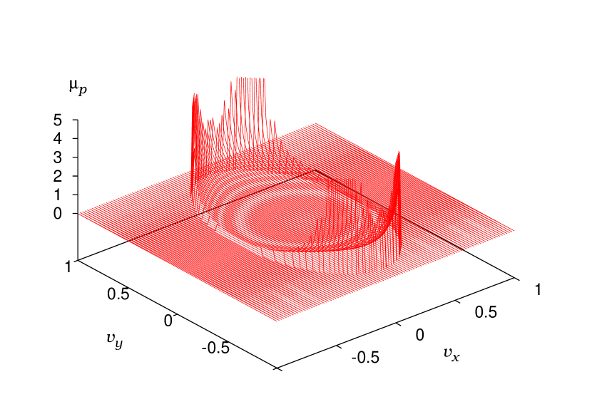
Figure 1: (Color online) The two-dimensional fundamental density-function $\mu_{p}(v_{x},v_{y})$ of limit distribution of pseudovelocities, when $p=1/4$.

III.2 Weight function ${\cal M}(v_{x},v_{y})$

Using (29), the weight function ${\cal M}(v_{x},v_{y})$ is explicitly determined as follows;

$${\cal M}(v_{x},v_{y})={\cal M}_{1}+{\cal M}_{2}v_{x}+{\cal M}_{3}v_{y}+{\cal M}_{4}v_{x}^{2}+{\cal M}_{5}v_{y}^{2}+{\cal M}_{6}v_{x}v_{y}$$ (35)

with

$$\mathcal{M}_{1} = \frac{1}{2}+\mathrm{Re}(q_{1}\bar{q}_{2}+q_{3}\bar{q}_{4}),$$

$$\mathcal{M}_{2} = -\Big{(}|q_{1}|^{2}-|q_{2}|^{2}\Big{)}+\frac{q}{\sqrt{\mathstrut pq}}\mathrm{Re}(q_{1}\bar{q}_{3}+q_{1}\bar{q}_{4}-q_{2}\bar{q}_{3}-q_{2}\bar{q}_{4}),$$

$$\mathcal{M}_{3} = -\Big{(}|q_{3}|^{2}-|q_{4}|^{2}\Big{)}+\frac{p}{\sqrt{\mathstrut pq}}\mathrm{Re}(q_{1}\bar{q}_{3}-q_{1}\bar{q}_{4}+q_{2}\bar{q}_{3}-q_{2}\bar{q}_{4}),$$

$$\mathcal{M}_{4} = \frac{1}{2}\Big{(}|q_{1}|^{2}+|q_{2}|^{2}-|q_{3}|^{2}-|q_{4}|^{2}\Big{)}-\frac{1+q}{p}\mathrm{Re}(q_{1}\bar{q}_{2})-\mathrm{Re}(q_{3}\bar{q}_{4})$$

$$- \frac{q}{\sqrt{\mathstrut pq}}\mathrm{Re}(q_{1}\bar{q}_{3}+q_{1}\bar{q}_{4}+q_{2}\bar{q}_{3}+q_{2}\bar{q}_{4}),$$

$$\mathcal{M}_{5} = -\frac{1}{2}\Big{(}|q_{1}|^{2}+|q_{2}|^{2}-|q_{3}|^{2}-|q_{4}|^{2}\Big{)}-\mathrm{Re}(q_{1}\bar{q}_{2})-\frac{1+p}{q}\mathrm{Re}(q_{3}\bar{q}_{4})$$

$$- \frac{p}{\sqrt{\mathstrut pq}}\mathrm{Re}(q_{1}\bar{q}_{3}+q_{1}\bar{q}_{4}+q_{2}\bar{q}_{3}+q_{2}\bar{q}_{4}),$$

$$\mathcal{M}_{6} = -\frac{1}{\sqrt{\mathstrut pq}}\mathrm{Re}(q_{1}\bar{q}_{3}-q_{1}\bar{q}_{4}-q_{2}\bar{q}_{3}+q_{2}\bar{q}_{4}),$$ (36)

where ${\rm Re}(z)$ denotes the real part of $z\in{\bf C}$ and $\overline{z}$ denotes the complex conjugate of $z\in{\bf C}$. The weight function defines the following real symmetric matrices ${\bf{M}}_{n}$, through the relations $\mathcal{M}_{n}=\phi^{\dagger}_{0}{\bf{M}}_{n}\phi_{0}$, $1\leq n\leq 6$,

$${\bf{M}}_{1} = \frac{1}{2}\left(\begin{array}[]{cccc}1&1&0&0\\ 1&1&0&0\\ 0&0&1&1\\ 0&0&1&1\end{array}\right),\quad{\bf{M}}_{2}=-\frac{1}{2\sqrt{\mathstrut pq}}\left(\begin{array}[]{cccc}2\sqrt{\mathstrut pq}&0&-q&-q\\ 0&-2\sqrt{\mathstrut pq}&q&q\\ -q&q&0&0\\ -q&q&0&0\end{array}\right),$$ (45)

$${\bf{M}}_{3} = -\frac{1}{2\sqrt{\mathstrut pq}}\left(\begin{array}[]{cccc}0&0&-p&p\\ 0&0&-p&p\\ -p&-p&2\sqrt{\mathstrut pq}&0\\ p&p&0&-2\sqrt{\mathstrut pq}\end{array}\right),\quad{\bf{M}}_{4}=-\frac{1}{2}\left(\begin{array}[]{cccc}-1&\frac{1+q}{p}&\frac{q}{\sqrt{pq}}&\frac{q}{\sqrt{pq}}\\ \frac{1+q}{p}&-1&\frac{q}{\sqrt{pq}}&\frac{q}{\sqrt{pq}}\\ \frac{q}{\sqrt{pq}}&\frac{q}{\sqrt{pq}}&1&1\\ \frac{q}{\sqrt{pq}}&\frac{q}{\sqrt{pq}}&1&1\end{array}\right),$$ (54)

$${\bf{M}}_{5} = -\frac{1}{2}\left(\begin{array}[]{cccc}1&1&\frac{p}{\sqrt{pq}}&\frac{p}{\sqrt{pq}}\\ 1&1&\frac{p}{\sqrt{pq}}&\frac{p}{\sqrt{pq}}\\ \frac{p}{\sqrt{pq}}&\frac{p}{\sqrt{pq}}&-1&\frac{1+p}{q}\\ \frac{p}{\sqrt{pq}}&\frac{p}{\sqrt{pq}}&\frac{1+p}{q}&-1\end{array}\right),\quad{\bf{M}}_{6}=\frac{1}{2\sqrt{\mathstrut pq}}\left(\begin{array}[]{cccc}0&0&-1&1\\ 0&0&1&-1\\ -1&1&0&0\\ 1&-1&0&0\end{array}\right).$$ (63)

Such matrix representations will be useful, when we generalize the present results to other models, whose quantum coins are given by larger matrices SKKK08 .

The integral $\int_{-\infty}^{\infty}dv_{x}\int_{-\infty}^{\infty}dv_{y}\mu_{p}(v_{x},v_{y}){\cal M}(v_{x},v_{y})$ is generally less than one, since the contributions from the eigenvalues $\lambda_{1}$ and $\lambda_{2}$ have not been included. The difference

$$\Delta=1-\int_{-\infty}^{\infty}dv_{x}\int_{-\infty}^{\infty}dv_{y}\mu_{p}(v_{x},v_{y}){\cal M}(v_{x},v_{y})$$ (64)

gives the weight of a point mass at $v_{x}=v_{y}=0$ in the distribution. That is, $\Delta$ gives the probability of localization around the origin of the present two-dimensional quantum walks IKK04 ; MKK07 (see Sec.III.D below).

III.3 Weak limit-theorem and symmetry of limit distribution

The result is summarized as the following limit theorem.

Theorem  Let

$$\nu(v_{x},v_{y})=\mu_{p}(v_{x},v_{y}){\cal M}(v_{x},v_{y})+\Delta\delta(v_{x})\delta(v_{y}),$$ (65)

where $\mu_{p}(v_{x},v_{y})$, ${\cal M}(v_{x},v_{y})$, and $\Delta$ are given by (34), (35) with (36), and (64), respectively, and $\delta(z)$ denotes Dirac’s delta function. Then

$$\lim_{t\to\infty}\left\langle\left(\frac{X_{t}}{t}\right)^{\alpha}\left(\frac{Y_{t}}{t}\right)^{\beta}\right\rangle=\int_{-\infty}^{\infty}dv_{x}\int_{-\infty}^{\infty}dv_{y}v_{x}^{\alpha}v_{y}^{\beta}\nu(v_{x},v_{y})$$ (66)

for all $\alpha,\beta=0,1,2,\cdots$.

As mentioned in an earlier paper MKK07 , distribution of quantum walks itself does not converge in the long-time limit, since time evolution of quantum system is simply given by a unitary transformation. The above theorem is regarded as a weak limit-theorem in the sense that, if we evaluate moments of pseudovelocity in oscillatory distributions of realized quantum walks, the results shall be converge to the values calculated by the formula (66) with the density function (65) in $t\to\infty$. If we integrate $\nu(v_{x},v_{y})$ over any region $D$ on a plane ${\bf R}^{2}$, then we obtain the probability that the pseudovelocity ${\bf V}_{t}=(X_{t}/t,Y_{t}/t)\in D$ in the $t\to\infty$ limit.

The polynomial form of (35) leads to the following classification of symmetry realized in the limit distribution.

(i)  When $\mathcal{M}_{3}=\mathcal{M}_{6}=0$, the limit of probability density $\nu(v_{x},v_{y})$ has the reflection symmetry for the $v_{x}$-axis; $\nu(v_{x},-v_{y})=\nu(v_{x},v_{y})$.

(ii)  When $\mathcal{M}_{2}=\mathcal{M}_{6}=0$, the limit of probability density $\nu(v_{x},v_{y})$ has the reflection symmetry for the $v_{y}$-axis; $\nu(-v_{x},v_{y})=\nu(v_{x},v_{y})$.

(iii)  When $\mathcal{M}_{2}=\mathcal{M}_{3}=\mathcal{M}_{6}=0$, the limit of probability density $\nu(v_{x},v_{y})$ has the reflection symmetries both for the $v_{x}$-axis and the $v_{y}$-axis; $\nu(v_{x},-v_{y})=\nu(-v_{x},v_{y})=\nu(v_{x},v_{y})$.

(iv)  When $\mathcal{M}_{2}=\mathcal{M}_{3}=0$, the limit of probability density $\nu(v_{x},v_{y})$ has the bi-rotational symmetry for the $v_{z}$-axis, which is perpendicular both to $v_{x}$- and $v_{y}$-axes; $\nu(-v_{x},-v_{y})=\nu(v_{x},v_{y})$.

III.4 Localization probability around the origin

By symmetry of the fundamental density-function (34), (64) with (35) becomes

$$\Delta=1-{\cal M}_{1}-{\cal M}_{4}K_{x}-{\cal M}_{5}K_{y}$$

with

$$K_{x} = \int_{-\infty}^{\infty}dv_{x}\int_{-\infty}^{\infty}dv_{y}\mu_{p}(v_{x},v_{y})v_{x}^{2},$$

$$K_{y} = \int_{-\infty}^{\infty}dv_{x}\int_{-\infty}^{\infty}dv_{y}\mu_{p}(v_{x},v_{y})v_{y}^{2}.$$

As shown in Appendix A, these integrals are readily performed and we obtain the following explicit expression for the probability of localization around the origin,

$$\Delta=1-{\cal M}_{1}-\frac{2}{\pi}(\arcsin\sqrt{p}-\sqrt{pq}){\cal M}_{4}-\frac{2}{\pi}(\arcsin\sqrt{q}-\sqrt{pq}){\cal M}_{5}.$$ (67)

The localization probability $\Delta$ is a function of the parameter $p\in(0,1)$ and an initial four-component qudit ${}^{T}\!\phi_{0}=(q_{1},q_{2},q_{3},q_{4})\in{\bf C}^{4},\sum_{j=1}^{4}|q_{j}|^{2}=1$ through (36). For example, (67) gives

$$\Delta=\frac{1}{\pi}(1-2\sqrt{pq})\left\{\frac{1}{p}\arcsin\sqrt{p}+\frac{1}{q}\arcsin\sqrt{q}-\frac{1}{\sqrt{pq}}\right\}$$

for ${}^{T}\!\phi_{0}=(1,1,-1,-1)/2$, and

$$\Delta=\frac{1}{\pi}(1+2\sqrt{pq})\left\{\frac{1}{p}\arcsin\sqrt{p}+\frac{1}{q}\arcsin\sqrt{q}-\frac{1}{\sqrt{pq}}\right\}$$

for ${}^{T}\!\phi_{0}=(1,1,1,1)/2$, respectively, where $q=1-p$. As shown in Fig.2, for ${}^{T}\!\phi_{0}=(1,1,-1,-1)/2$, the localization probability $\Delta$ attains the minimum $=0$ for the Grover-walk model, $p=q=1/2$, while for ${}^{T}\!\phi_{0}=(1,1,1,1)/2$, it attains the maximum $=2(\pi-2)/\pi=0.726\cdots$ for the Grover-walk model.

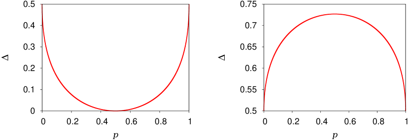
Figure 2: (Color online) Dependence of localization probability around the origin $\Delta$ on the parameter $p\in(0,1)$. (a) The case ${}^{T}\!\phi_{0}=(1,1,-1,-1)/2$. When $p=1/2$ (the Grover-walk model), $\Delta=0$. (b) The case ${}^{T}\!\phi_{0}=(1,1,1,1)/2$. When $p=1/2$ (the Grover-walk model), $\Delta=2(\pi-2)/\pi=0.726\cdots$.

If we make the initial qudit depend on the parameter as

$${}^{T}\!\phi_{0}=\left(\sqrt{\frac{p}{2}},\sqrt{\frac{p}{2}},-\sqrt{\frac{q}{2}},-\sqrt{\frac{q}{2}}\right),\quad q=1-p,$$ (68)

for example, then $\Delta\equiv 0$ for ${\cal M}_{1}=1,{\cal M}_{4}={\cal M}_{5}=0$, and thus the quantum walker is extended with probability one for all $p\in(0,1)$.

It should be noted that $\Delta$ is defined as the intensity of Dirac’s delta-function at the origin found in the limit density-function of pseudovelocity (see Eq.(65)). It implies that $\Delta$ gives the probability that the quantum walker loses its velocity and stays around the starting point, i.e. the origin. Therefore, $\Delta$ is, in general, greater than the time-averaged probability that the walker stays exactly at the starting point, $\overline{P}_{\infty}$, which was calculated in IKK04 . For example, for the Grover-walk model with the initial qudit ${}^{T}\!\phi_{0}=(1,1,1,1)/2$, $\Delta=2(\pi-2)/\pi=0.726\cdots$, as mentioned above, while $\overline{P}_{\infty}=2\{(\pi-2)/\pi\}^{2}=0.264...$ as reported in Sec.V.C in IKK04 .

IV COMPARISON WITH COMPUTER SIMULATIONS

In order to demonstrate the validity of the above results, here we show comparison with numerical results of direct computer simulations MKK07 . In Figs.3-6, the left figures show the distribution of pseudovelocity ${\bf V}_{t}=(X_{t}/t,Y_{t}/t)$ at time step $t=30$ numerically obtained by computer simulations and the right figures the long-time limits of probability densities $\nu(v_{x},v_{y})$ determined by our theorem. The four figures show the symmetries (i)-(iv) classified in Sec.III.C. In all of these four cases shown in Figs.3-6, $\Delta>0$ and we can see a peak at the origin in each right figure (b), which indicates the contribution $\Delta\delta(v_{x})\delta(v_{y})$ in the limit density-function (65).

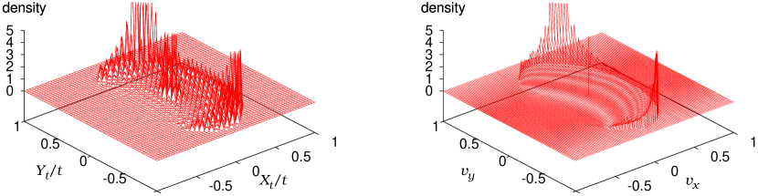
Figure 3: (Color online) The case $p=1/4$ and ${}^{T}\!\phi_{0}=(1,-1,1,1)/2$. Since $\mathcal{M}_{3}=\mathcal{M}_{6}=0$ in this case, the limit distribution has the reflection symmetry for the $v_{x}$-axis; $\nu(v_{x},-v_{y})=\nu(v_{x},v_{y})$. (a) Distribution of pseudovelocity ${\bf V}_{t}=(X_{t}/t,Y_{t}/t)$ at time step $t=30$ numerically obtained by computer simulation. (b) Probability density of limit distribution.

Figure 4: (Color online) The case $p=1/4$ and ${}^{T}\!\phi_{0}=(1,1,1,-1)/2$. Since $\mathcal{M}_{2}=\mathcal{M}_{6}=0$ in this case, the limit distribution has the reflection symmetry for the $v_{y}$-axis; $\nu(-v_{x},v_{y})=\nu(v_{x},v_{y})$. (a) Distribution of pseudovelocity ${\bf V}_{t}=(X_{t}/t,Y_{t}/t)$ at time step $t=30$ numerically obtained by computer simulation. (b) Probability density of limit distribution.

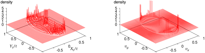
Figure 5: (Color online) The case $p=1/4$ and ${}^{T}\!\phi_{0}=(1,1,0,0)/\sqrt{2}$. Since $\mathcal{M}_{2}=\mathcal{M}_{3}=\mathcal{M}_{6}=0$ in this case, the limit distribution has the reflection symmetries both for the $v_{x}$-axis and the $v_{y}$-axis; $\nu(v_{x},-v_{y})=\nu(-v_{x},v_{y})=\nu(v_{x},v_{y})$. (a) Distribution of pseudovelocity ${\bf V}_{t}=(X_{t}/t,Y_{t}/t)$ at time step $t=30$ numerically obtained by computer simulation. (b) Probability density of limit distribution.

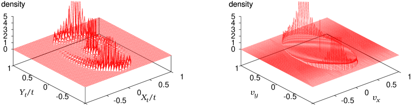
Figure 6: (Color online) The case $p=1/4$ and ${}^{T}\!\phi_{0}=(1,-1,-1,1)/2$. Since $\mathcal{M}_{2}=\mathcal{M}_{3}=0$ in this case, the limit distribution has the bi-rotational symmetry for the $v_{z}$-axis, which is perpendicular both to $v_{x}$- and $v_{y}$-axes; $\nu(-v_{x},-v_{y})=\nu(v_{x},v_{y})$ (a) Distribution of pseudovelocity ${\bf V}_{t}=(X_{t}/t,Y_{t}/t)$ at time step $t=30$ numerically obtained by computer simulation. (b) Probability density of limit distribution.

We observe oscillatory behavior in distributions of ${\bf V}_{t}=(X_{t}/t,Y_{t}/t)$ in computer simulations. In general, as the time step $t$ increases, the frequency of oscillation becomes higher, but, if we smear out the oscillatory behavior, the averaged values of distribution shall be well-described by the density functions of limit distributions (65), which is the phenomenon implied by our weak limit-theorem MKK07 .

V CONCLUDING REMARKS

In general, quantum coins, which determine time-evolution of quantum walkers with spatial shift-operators, are given by unitary transformations BCA03 ; MKK07 . The set of all $N\times N$ unitary matrices makes a group, the unitary group U($N$), whose dimension is $N^{2}$ (see, for example, Geo99 ). Though the determinant of unitary matrix is generally given by $e^{i\varphi},\varphi\in[-\pi/2,\pi/2)$, this global phase factor of quantum coin is irrelevant in calculating any moments of walker’s positions in quantum-walk models KFK05 . For example, in the standard two-component ($N=2$) quantum walks, the number of relevant parameters to specify a quantum coin is $N^{2}-1=2^{2}-1=3$ (Cayley-Klein parameters), and the dependence of limit distributions of pseudovelocities on the three parameters was completely determined Kon02 ; Kon05 ; Kon07 ; KFK05 ; MKK07 . In the present paper we have considered a one-parameter family of unitary matrices (13) in U(4) as quantum coins. The present study should be extended to more general models, whose U(4)-quantum coins are fully controlled by $4^{2}-1=15$ parameters.

One of the motivations to study the present family of models in this paper is the fact that it contains the Grover walk on the plane. It will be interesting and important to derive limit distributions of pseudovelocities of quantum walkers on variety of plane lattices different from the square lattices and in the higher-dimensional lattices CLXGKK05 . For example, the quantum coin of the Grover walk in the $D$-dimensional hyper-cubic lattice is given by the $2D\times 2D$ orthogonal matrix $A^{(D)}=(A^{(D)}_{jk})$ with the elements

$$A^{(D)}_{jk}=\Bigg{\{}\begin{array}[]{ll}1/D-1,&\mbox{if $j=k$}\cr 1/D,&\mbox{if $j\not=k$}.\end{array}$$ (69)

It is also an interesting problem to relate the present results to solutions of the continuous-time quantum-walk models on two-dimensional lattices MVB05 .

At the end of the present paper, we refer to the fact that recent papers propose implementations of not only one-dimensional but also two-dimensional quantum walks using optical equipments RS05 ; EMBL05 , ion-trap systems FOBH05 , and ultra-cold Rydberg atoms in optical lattices CREG06 ; MBA07 . We hope that combinations of experiments and theoretical works of quantum physics will make significant contribution to development of quantum informatics.

Appendix A On Integrals

Consider the integral

$$I=\int_{-\infty}^{\infty}dv_{x}\int_{-\infty}^{\infty}dv_{y}{\bf 1}_{\{v_{x}^{2}/p+v_{y}^{2}/q<1\}}\frac{1}{(v_{x}+v_{y}+1)(v_{x}-v_{y}+1)(v_{x}+v_{y}-1)(v_{x}-v_{y}-1)}$$

with $p+q=1,p,q\geq 0$. Let

$$v_{x}=\sqrt{p}r\frac{1}{2}\left(z+\frac{1}{z}\right),\quad v_{y}=\sqrt{q}r\frac{1}{2i}\left(z-\frac{1}{z}\right).$$ (70)

Then

$$I=-2^{4}i\sqrt{pq}\int_{0}^{1}dr\frac{J(r)}{r^{3}}$$

with a contour integral on a complex plane ${\bf C}$,

$$J(r)=\oint_{C_{0}}dzf(z),$$

where

$$f(z)=\frac{z^{3}}{(z+z_{+})(z+z_{-})(z-z_{+})(z-z_{-})(z+\overline{z_{+}})(z+\overline{z_{-}})(z-\overline{z_{+}})(z-\overline{z_{-}})}$$ (71)

with

$$z_{\pm}=(\sqrt{p}+i\sqrt{q})\frac{1}{r}(1\pm\sqrt{1-r^{2}}).$$

Here $C_{0}$ denotes the unit circle centered at the origin on ${\bf C}$, $|z|=1$. There are four simple poles at $z=z_{-},\overline{z_{-}},-z_{-}$ and $-\overline{z_{-}}$ inside of the contour $C_{0}$ and the Cauchy residue theorem can be applied (see, for example, Chapter 4 in AF03 ) to obtain

$$J(r)=2\pi i\Big{\{}{\rm Res}(f,z_{-})+{\rm Res}(f,\overline{z_{-}})+{\rm Res}(f,-z_{-})+{\rm Res}(f,-\overline{z_{-}})\Big{\}},$$

where we see

$${\rm Res}(f,z_{-}) = (z-z_{-})f(z)\Big{|}_{z=z_{-}}$$

$$= \frac{r^{4}}{2^{7}\sqrt{pq}\sqrt{1-r^{2}}}\frac{(\sqrt{p}+i\sqrt{q}\sqrt{1-r^{2}})(\sqrt{q}-i\sqrt{p}\sqrt{1-r^{2}})}{(1-pr^{2})(1-qr^{2})}$$

and ${\rm Res}(f,-z_{-})={\rm Res}(f,z_{-})$, ${\rm Res}(f,-\overline{z_{-}})={\rm Res}(f,\overline{z_{-}})=\overline{{\rm Res}(f,z_{-})}$. We obtain

$$J(r)=\frac{\pi i}{2^{4}}\frac{r^{4}}{\sqrt{1-r^{2}}}\left\{\frac{1}{1-pr^{2}}+\frac{1}{1-qr^{2}}\right\}.$$

The integral formula

$$\int_{0}^{1}dx\frac{x}{(1-a^{2}x^{2})\sqrt{1-x^{2}}}=\frac{\arcsin a}{a\sqrt{1-a^{2}}},\quad|a|<1$$ (72)

is useful and we arrive at the result

$$I=\pi(\arcsin\sqrt{p}+\arcsin\sqrt{q})=\frac{\pi^{2}}{2}.$$

It implies that $\mu_{p}(v_{x},v_{y})$ given by (34) is well-normalized; $\int_{-\infty}^{\infty}dv_{x}\int_{-\infty}^{\infty}dv_{y}\mu_{p}(v_{x},v_{y})=I\times 2/\pi^{2}=1$.

Similarly, we can also calculate the integrals

$$I_{x} = \int_{-\infty}^{\infty}dv_{x}\int_{-\infty}^{\infty}dv_{y}{\bf 1}_{\{v_{x}^{2}/p+v_{y}^{2}/q<1\}}\frac{v_{x}^{2}}{(v_{x}+v_{y}+1)(v_{x}-v_{y}+1)(v_{x}+v_{y}-1)(v_{x}-v_{y}-1)},$$

$$I_{y} = \int_{-\infty}^{\infty}dv_{x}\int_{-\infty}^{\infty}dv_{y}{\bf 1}_{\{v_{x}^{2}/p+v_{y}^{2}/q<1\}}\frac{v_{y}^{2}}{(v_{x}+v_{y}+1)(v_{x}-v_{y}+1)(v_{x}+v_{y}-1)(v_{x}-v_{y}-1)}.$$

By the change of integral variables (70), we have

$$I_{x}=-2^{2}ip\sqrt{pq}\int_{0}^{1}dr\frac{J_{x}(r)}{r},\quad I_{y}=2^{2}iq\sqrt{pq}\int_{0}^{1}dr\frac{J_{y}(r)}{r}$$

with

$$J_{x}(r)=\oint_{C_{0}}dzf_{x}(z),\quad J_{y}(r)=\oint_{C_{0}}dzf_{y}(z),$$

where $f_{x}(z)=(z+1/z)^{2}f(z)$ and $f_{y}(z)=(z-1/z)^{2}f(z)$ with (71). The Cauchy residue theorem gives

$$J_{x}(r)=\frac{\pi i}{2^{2}}\frac{r^{4}}{(1-pr)\sqrt{1-r^{2}}},\quad J_{y}(r)=-\frac{\pi i}{2^{2}}\frac{r^{4}}{(1-qr)\sqrt{1-r^{2}}}.$$

The integral formula (72) and the fact $\int_{0}^{1}drr/\sqrt{1-r^{2}}=1$ lead to the results

$$I_{x} = \pi(\arcsin\sqrt{p}-\sqrt{pq}),$$

$$I_{y} = \pi(\arcsin\sqrt{q}-\sqrt{pq}).$$

Since $K_{x}=I_{x}\times(2/\pi^{2})$ and $K_{y}=I_{y}\times(2/\pi^{2})$, they give the expression (67).

It is interesting to see that the above calculation of the integral $I$ gives the following identity,

$$\frac{1}{2}\int_{-\infty}^{\infty}dv_{x}\int_{-\infty}^{\infty}dv_{y}\mu_{p}(v_{x},v_{y})=\int_{0}^{\infty}dr\,r\mu(r;\sqrt{p})+\int_{0}^{\infty}dr\,r\mu(r;\sqrt{q}),$$ (73)

where $\mu(x;a)$ is the Konno density-function of one-dimensional quantum walk Kon02 ; Kon05 ; KFK05 ; MKK07 ; SKKK08

$$\mu(x;a)=\frac{\sqrt{1-a^{2}}}{\pi(1-x^{2})\sqrt{a^{2}-x^{2}}}{\bf 1}_{\{|x|<|a|\}}.$$

References

- (1) B. C. Travaglione and G. J. Milburn, Phys. Rev. A 65, 032310 (2002)
- (2) J. Kempe, Contemp. Phys. 44, 307 (2003).
- (3) A. Ambainis, Int. J. Quantum Inf. 1, 507 (2003).
- (4) T. A. Brun, H. A. Carteret, and A. Ambainis, Phys. Rev. A 67, 052317 (2003).
- (5) V. M. Kendon, Int. J. Quantum Inf. 4, 791 (2006).
- (6) Y. Aharonov, L. Davidovich, and N. Zagury, Phys. Rev. A 48, 1687 (1993).
- (7) D. A. Meyer, J. Stat. Phys. 85, 551 (1996).
- (8) A. Nayak and A. Vishwanath, e-print quant-ph/0010117.
- (9) A. Ambainis, E. Bach, A. Nayak, A. Vishwanath, and J. Watrous, in Proceedings of the 33rd Annual ACM Symposium on Theory of Computing (ACM Press, New York, 2001), pp.37-49.
- (10) N. Konno, Quantum Walks, Lecture at the School “Quantum Potential Theory: Structure and Applications to Physics” held at the Alfried Krupp Wissenschaftskolleg, Greifswald, 26 February - 9 March 2007. (Reihe Mathematik, Ernst-Moritz-Arndt-Universität Greifswald, No.2, 2007.) The lecture note is available at http://www.math-inf.uni-greifswald.de/algebra/qpt/konno-26nov2007, and will be published in Springer Lecture Notes in Mathematics.
- (11) Precisely speaking, the theory of quantum walks has been divided into the discrete-time version and the continuous-time version. In the present paper we focus on the discrete-time models. The study on the connection of these two versions is itself interesting and important. See, for example, F. W. Strauch, Phys. Rev. A 74, 030301(R) (2006).
- (12) N. Konno, Quantum Inf. Process 1, 345 (2002).
- (13) N. Konno, J. Math. Soc. Jpn, 57, 1179 (2005).
- (14) G. Grimmett, S. Janson, and P. F. Scudo, Phys. Rev. E 69, 026119 (2004).
- (15) M. Katori, S. Fujino, and N. Konno, Phys. Rev. A 72, 012316 (2005).
- (16) T. Miyazaki, M. Katori, and N. Konno, Phys. Rev. A 76, 012332 (2007).
- (17) M. Sato, N. Kobayashi, M. Katori and N. Konno, e-print quant-ph/0802.1997.
- (18) T. D. Mackay, S. D. Bartlett, L. T. Stephenson, and B. C. Sanders, J. Phys. A: Math. Gen. 35, 2745 (2002).
- (19) B. Tregenna, W. Flanagan, R. Maile, and V. Kendon, New J. Phys. 5, 83 (2003).
- (20) I. Carneiro, M. Loo, X. Xu, M. Girerd, V. Kendon, and P. L. Knight, New J. Phys. 7, 156 (2005).
- (21) S. E. Venegas-Andraca, J. L. Ball, K. Burnett, and S. Bose, New J. Phys. 7, 221 (2005).
- (22) O. Mülken, A. Volta, and A. Blumen, Phys. Rev. A 72, 042334 (2005).
- (23) L. K. Grover, Phys. Rev. Lett. 79, 325 (1997).
- (24) N. Shenvi, J. Kempe and K. Birgitta Whaley, Phys. Rev. A 67, 052307 (2003).
- (25) A. M. Childs and J. Goldstone, Phys. Rev. A 70, 022314 (2004).
- (26) A. M. Childs and J. Goldstone, Phys. Rev. A 70, 042312 (2004).
- (27) A. Tulsi, e-print quant-ph/0801.0497.
- (28) N. Inui, Y. Konishi, and N. Konno, Phys. Rev. A 69, 052323 (2004).
- (29) Localization of quantum walk studied by Inui et al. and in the present paper is not directly related to the Anderson localization. If we consider quantum walks with disorder, however, the process is closely related to Anderson’s model. In the continuous-time quantum-walk version, the Anderson localization was discussed in O. Mülken, V. Bierbaum, and A. Blumen, Phys. Rev. E 75, 031121 (2007).
- (30) A. C. Oliveira, R. Portugal and R. Donangelo, Phys. Rev. A 74, 012312 (2006).
- (31) H. Georgi, Lie Algebras in Particle Physics, 2nd ed. (Perseus Books, Reading, 1999).
- (32) E. Roldán and J. C. Soriano, J. Mod. Opt. 52, 2649 (2005).
- (33) K. Eckert, J. Mompart, G. Birkl, and M. Lewenstein, Phys. Rev. A 72, 012327 (2005).
- (34) S. Fujiwara, H. Osaki, I. M. Buluta, and S. Hasegawa, Phys. Rev. A 72, 032329 (2005).
- (35) R. Côté, A. Russell, E. E. Eyler, and P. L. Gould, New J. Phys. 8, 156 (2006).
- (36) O. Mülken, A. Blumen, T. Amthor, C. Giese, M. Reetz-Lamour, and M. Weidemüller, Phys. Rev. Lett. 99, 090601 (2007).
- (37) M. J. Ablowitz and A. S. Fokas, Complex Variables, Introduction and Applications, 2nd ed. (Cambridge University Press, 2003).