The Valence Bond Glass phase

Abstract

We show that a new glassy phase can emerge in presence of strong magnetic frustration and quantum fluctuations. It is a Valence Bond Glass. We study its properties solving the Hubbard-Heisenberg model on a Bethe lattice within the large $N$ limit introduced by Affleck and Marston. We work out the phase diagram that contains Fermi liquid, dimer and valence bond glass phases. This new glassy phase has no electronic or spin gap (although a pseudo-gap is observed), it is characterized by long-range critical valence bond correlations and is not related to any magnetic ordering. As a consequence it is quite different from both valence bond crystals and spin glasses.

The interplay of strong quantum fluctuations and geometrically frustrated magnetic interactions can give rise to new low temperature phases. As noticed by Anderson [1] a way to minimize the effect of frustration and obtain a low energy state is coupling the electrons in valence bonds. A very good variational wave function that is generically in competition with the antiferromagnetic (or more general magnetic) state can be obtained by forming a superposition of short range valence bonds that are arranged as dimers on the lattice. If no lattice symmetry is broken this corresponds to the (so called) resonating valence bond liquid (RVBL). In the last decades, this state has received a lot of attention in connection with the unusual physical behavior of the normal phase of underdoped high $T_{c}$ superconductors [2]. Indeed Anderson [3] proposed that the holes created by doping the antiferromagnetic insulator (of the high $T_{c}$’s phase diagram) can gain substantial kinetic energy in the RVBL state and not in an antiferromagnetic background. As a consequence, doping favors the RVBL state which could then become the thermodynamic stable phase and be responsible for the unusual behavior of underdoped samples. Concomitantly, resonating valence bond ground states have been the focus of an intense activity [4] in the context of frustrated magnets. RVBL or spin liquids have been found for several models [4]. These states can undergo quantum phase transitions where lattice symmetries are spontaneously broken. This gives rise to valence bond crystals (VBC). Different models are known to lead to this type of ground states [4] characterized by long range dimer-dimer correlations. The situation in experiments is complicated by unavoidable magneto-elastic couplings: making the difference between induced and spontaneous dimerization is a difficult task. A first experimental example of spontaneously broken states has been apparently found in [5].
The aim of this work is to study a new kind of valence bond state: the valence bond glass (VBG). Similarly to VBC the arrangement of the dimers (or valence bonds) breaks the lattice symmetry. However, contrary to VBC, this corresponds to an amorphous dimerization and not crystalline one. Although VBG are analogous to spin glasses [6] they are physically quite different. In particular the spins do not freeze in a disordered profile. We expect that the VBG phase can arise in presence of strong magnetic frustration as one of the competing ground states. The addition of (little) quenched disorder will favor this phase. Depending on the system, the low temperature phase could be either a VBG or a spin glass. Actually, the spin glass phase is conjectured to exist even in absence of disorder on some frustrated lattices [7] (see however [8, 9]).
In the following we shall investigate the properties of the valence bond glass phase focusing on the Hubbard-Heisenberg model within the large $N$ approximation introduced by Affleck and Marston [10]. The underlying lattice we shall focus on is a random regular graph with connectivity $z$. The reason for this choice is twofold. First, this type of graphs are on any finite lengthscale as Bethe lattices or Cayley trees. This, as it is well known for classical systems [11], introduces useful simplification in the analysis of the model. The main reason is, however, that topological frustration and quenched disorder are introduced by very long loops (of the order $\log{\cal N}$ where ${\cal N}$ is the number of sites) in random regular graphs. These loops disfavor crystalline states and let emerge easily the glassy phases [12, 13]. We consider the $SU(N)$ version of the Hubbard-Heisenberg model introduced in [10]:

$${\cal H} = -t\sum_{\langle i,j\rangle}\left(c^{\dagger}_{i,\alpha}c_{j,\alpha}+\textrm{h.c.}\right)+\frac{U}{N}\sum_{i}\left(n_{i}-\frac{N}{2}\right)^{2}$$ (1)

$$\qquad+\,\frac{J}{N}\sum_{\langle i,j\rangle}\mathbf{S}_{i}\cdot\mathbf{S}_{j},$$

where $c_{i,\alpha}$ denotes the destruction operator of an electron of spin index $\alpha$ ($\alpha=1,\ldots,N$ with $N$ even) on the site $i$. The sum $\langle i,j\rangle$ is restricted on nearest neighbor sites on the lattice. The first two terms correspond to the $SU(N)$ Hubbard model, while the last term accounts for the nearest neighbor antiferromagnetic interaction ($J>0$). We shall focus on the $N\rightarrow\infty$ limit and consider only the half-filling case, where $n_{i}/(N/2)=\sum_{\alpha}c^{\dagger}_{i,\alpha}c_{i,\alpha}/(N/2)=1$ for all sites. Using that ${\bf S}_{i}\cdot{\bf S}_{j}$ equals $-\sum_{\alpha,\beta}c^{\dagger}_{i,\alpha}c_{j,\alpha}c^{\dagger}_{j,\beta}c_{i,\beta}$ up to constant terms in the large $N$ limit [10, 14], the Hamiltonian can be rewritten in a $SU(N)$ manifestly invariant form. At half-filling it reads:

$${\cal H}=-t\sum_{\langle i,j\rangle}\left(c^{\dagger}_{i,\alpha}c_{j,\alpha}+\textrm{h.c.}\right)-\frac{J}{N}\sum_{\langle i,j\rangle}c^{\dagger}_{i,\alpha}c_{j,\alpha}c^{\dagger}_{j,\beta}c_{i,\beta}.$$ (2)

Note that all terms constant in the large $N$ limit have been neglected. Here and henceforth the summation over the $SU(N)$ indices will be skipped for simplicity. The partition function of the system at finite temperature can be written as a path integral

$$Z=\int\!{\cal D}c\,{\cal D}c^{\dagger}\exp\left[-\int_{0}^{\beta}\!\textrm{d}\tau\,{\cal L}(c,c^{\dagger})\right],$$ (3)

where $\beta$ is the inverse temperature, and the (imaginary time) Lagrangian is ${\cal L}(c,c^{\dagger})={\cal H}+\sum_{i}c^{\dagger}_{i,\alpha}\left(\textrm{d}/\textrm{d}\tau\right)c_{i,\alpha}$. The functional integral is of course non trivial, due to the presence of the non linear interaction. However, one can perform a Hubbard-Stratonovich transformation which allows to rewrite the Lagrangian quadratically in the fermions, at the expense of introducing a new (complex) bosonic field, $\chi_{ij}$, on each edge of the lattice [10]:

$${\cal L}(c,c^{\dagger},\chi) = \sum_{\langle i,j\rangle}\left\{\frac{N}{J}|\chi_{ij}|^{2}-\left[\left(t+\chi_{ij}\right)c^{\dagger}_{i,\alpha}c_{j,\alpha}+\textrm{h.c.}\right]\right\}$$ (4)

$$\qquad+\,\sum_{i}c^{\dagger}_{i,\alpha}\left(\frac{\textrm{d}}{\textrm{d}\tau}\right)c_{i,\alpha}.$$

The equation of motion of the auxiliary bosonic field reads:

$$\langle\chi_{ij}(\tau)\rangle=\,\frac{J}{N}\langle c^{\dagger}_{j,\alpha}(\tau)c_{i,\alpha}(\tau)\rangle.$$ (5)

$\chi_{ij}$ is the valence bond field and gives an extra contribution to the electron hopping amplitude between the sites $i$ and $j$. The number of valence bonds on link $(ij)$ is given by $N|\chi_{ij}|^{2}/J$ up to subleading terms [10].
The advantage of this representation is that the integral over the fermionic degrees of freedom is now Gaussian. Therefore, they can be integrated out, leading to an effective action which depends only on the bosonic variables:

$$\exp\left[-S_{eff}(\chi)\right]=\int\!{\cal D}c\,{\cal D}c^{\dagger}\exp\left[-\int_{0}^{\beta}\!\!\textrm{d}\tau\,{\cal L}(c,c^{\dagger},\chi)\right].$$ (6)

The effective action thus reads:

$$S_{eff}=N\int_{0}^{\beta}\!\!\textrm{d}\tau\sum_{\langle i,j\rangle}\frac{1}{J}|\chi_{ij}|^{2}-N\textrm{Tr}\,\log{\mathbb{M}},$$ (7)

where the matrix ${\mathbb{M}}$ is given by ${\mathbb{M}}=[(\textrm{d}/\textrm{d}\tau){\mathbb{I}}-t\mathbb{C}-\hat{\chi}]$, $\mathbb{C}$ being the connectivity matrix of the lattice, i.e., $\mathbb{C}_{ij}=1$ if $i$ and $j$ are nearest neighbors on the lattice and zero otherwise. $\hat{\chi}$ has an analogous definition except that $\hat{\chi}_{ij}=\chi_{ij}$ if $i$ and $j$ are nearest neighbors.
So far, these transformations are exact and do not depend on the particular choice of the lattice. In the $N\to\infty$ limit the saddle point integration over the bosonic variables, $\chi_{ij}$, becomes exact and we can compute the free energy of the system by seeking the lowest minimum of the effective action. Assuming that at the saddle point the valence bond operators are time-independent, the problem reduces to finding the minima of the “classical” free energy $\beta F(\chi)=S_{eff}/N$ (N being the number of SU(N) indices),

$$F(\chi)=\sum_{\langle i,j\rangle}\frac{1}{J}|\chi_{ij}|^{2}-\frac{1}{\beta}\sum_{\lambda}\log\left[1+\exp\left(-\beta\lambda\right)\right]\quad.$$ (8)

We denote by $\lambda$ the eigenvalues of the one-particle Hamiltonian

$${\cal H}_{1}=-\sum_{\langle i,j\rangle}\left[\left(t+\chi_{ij}\right)c^{\dagger}_{i}c_{j}+\textrm{h.c.}\right]\quad.$$ (9)

Note that the (complex) bosonic variables $\chi_{ij}$ can have any arbitrary spatial dependence and that there is no need to introduce the chemical potential since it is expected, and found, to be zero at half filling. For simplicity we will set $J=1$ in the following, bearing in mind that all energy scales are measured in units of $J$.
The saddle point equations consist simply in Eq. (5) where the average on the RHS is performed using the Hamiltonian ${\cal H}_{1}$. Obtaining an analytical solution for a given particular lattice is, in general, a hard task. However, in some special cases, the problem can be simplified. In particular by considering periodic solutions one reduces the independent degrees of freedom to a finite number ($4$ in the case studied by Affleck and Marston [10]). Our aim is to find whether there are amorphous or chaotic solutions. Thus, in our case, obtaining a full analytical solution seems extremely difficult.
On infinite random graphs the Bethe-Peierls approximation is exact [12]: since the average length of the loops is infinite, it is possible to write down self-consistent iteration equations for local “cavity” Green’s functions, (or “Weiss functions”), ${\cal G}_{i}$, defined on each site of the graph [15]. In particular, for any given configuration of the valence bonds, $\{\chi_{ij}\}$, it is straightforward to show that the following recursion relations must hold:

$${\cal G}_{i}(\nu_{n})=i\nu_{n}-\sum_{j}^{z-1}\frac{|t+\chi_{ij}|^{2}}{{\cal G}_{j}(\nu_{n})},$$ (10)

where $\nu_{n}=(2n+1)\pi/\beta$ are the fermionic Matsubara frequencies. The Green’s function, $G_{i}(\nu_{n})=-\beta\langle c_{i\alpha}(\nu_{n})c_{i\alpha}^{\dagger}(\nu_{n})\rangle$, can be calculated on each site as a function of the ${\cal G}_{i}$ on the neighboring sites, by using Eq. (10), where the sum is extended over all the $z$ neighbors. For any given finite graph, and for any given profile of the bosonic field, Eqs. (10) provide a set of solvable equations for the cavity propagators. Furthermore, by enforcing the equation of motion for the valence bonds, Eq. (5), one finds that, on each link of the graph, the bosonic operators must verify:

$$\chi_{ij}=-\,\frac{1}{\beta}\sum_{n}\frac{t+\chi_{ij}}{{\cal G}_{i}(\nu_{n}){\cal G}_{j}(\nu_{n})-|t+\chi_{ij}|^{2}}.$$ (11)

The last equation is non-local, and is reminiscent of the TAP equations derived in the context of spin glasses [17]. For infinite systems Eqs. (10) and (11) allow to treat the liquid and the dimer phase (see below) in a very natural way. The analysis in the glass phase is much more involved and complicated. See [12] for the method used in classical cases and [16] for its extension to quantum cases. As a consequence we will use the previous approach to study simple (non disordered) phases and the transition lines. In order to study the glassy phase we interpret the free energy, Eq. (8), as the Hamiltonian of a classical system of complex variables. Hence, the problem of finding the minima of the free energy is reduced to finding classical ground states. To solve the latter problem we use Monte Carlo annealing simulations. Basically, we introduce an auxiliary temperature $T_{aux}$ and, at each step, we attempt to change one $\chi_{ij}$ at random according to the Boltzmann weight $e^{-F(\chi)/T_{aux}}$. The move is accepted with probability $p=\textrm{min}\left\{1,\exp[-\Delta F/T_{aux}]\right\}$. The auxiliary temperature is finally decreased at constant rate down to zero temperature. Details on the numerical procedure are discussed in the Appendix.

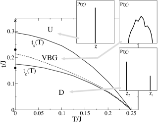
Figure 1: Phase diagram of the Hubbard-Heisenberg $SU(N)$ model at half filling on the random regular graph ($z=3$). We show the relative positions of the uniform phase (U), the dimer phase (D), and the valence bond glass (VBG). At $t_{s}(T)$ the uniform phase becomes unstable, the valence bond non-linear susceptibility diverges (see Fig. 3), and a continuous transition from the Fermi liquid to the VBG takes place. At $t_{c}(T)$ the free energies of the dimer phase and that of the VBG coincide and a first-order transition occurs. The dashed line corresponds to the spinodal of the dimer phase. The probability distributions of the valence bonds in the different phases are reproduced schematically in the insets.

By employing both the analytical and the numerical approaches described above, we have derived the phase diagram of the $SU(N)$ Hubbard-Heisenberg model on the random regular graph with connectivity $z=3$, see Fig. 1.
Uniform phase—At high enough temperature and hopping amplitude the system is in a uniform phase, where the bond operators are real and equal on each link of the graph, $\chi_{ij}=\chi$. For a given value of $\chi$, the electronic density of states can be computed easily since the density of states of the connectivity matrix is known  [18], see the inset of Fig. 2. The uniform phase is translational invariant and gapless. It is clearly a Fermi liquid.
For each value of $T$ and $t$, $\chi(T,t)$ in the uniform phase can be computed within the Bethe approximation, by enforcing translational invariance into Eqs. (10) and (11) (i.e., ${\cal G}_{i}={\cal G}$ and $\chi_{ij}=\chi$), which reduce to a simple algebraic equation:

$$\chi=\sum_{n}\frac{(t+\chi)/\beta}{\frac{\nu_{n}^{2}}{2}+(z-2)|t+\chi|^{2}+\nu_{n}\sqrt{\frac{\nu_{n}^{2}}{4}+(z-1)|t+\chi|^{2}}}.$$ (12)

One can then check the stability of the liquid solution with respect to any other solution of the bosonic field. This amounts in studying the (lowest) eigenvalues of the Hessian of $F(\chi)$. Using the base where the one-particle Hamiltonian, Eq. (9), is diagonal, and Fourier transforming with respect to the imaginary time, one gets

$$\!\!\!\!\!\!\!\!\!\!\!\!\!\!\!\frac{\partial^{2}F(\chi)}{\partial\chi_{ij}(\omega_{n})\partial\chi^{\star}_{kl}(\omega_{n})}=\frac{1}{J}\,\delta_{(i,j)(l,m)}-\sum_{\lambda,\lambda^{\prime}}v_{\lambda}^{i}v_{\lambda}^{j}v_{\lambda^{\prime}}^{l}v_{\lambda^{\prime}}^{k}$$ (13)

$$\,\,\,\,\,\,\,\,\,\,\,\times\,\frac{1-e^{\beta(\lambda+\lambda^{\prime})}}{1+e^{\beta\lambda}+e^{\beta\lambda^{\prime}}+e^{\beta(\lambda+\lambda^{\prime})}}\,\frac{\lambda+\lambda^{\prime}}{\omega_{n}^{2}+\left(\lambda+\lambda^{\prime}\right)^{2}},$$

where $v_{\lambda}^{i}$ is the $i$-th component of the eigenvector associated with the eigenvalue $\lambda$, and $\omega_{n}=2n\pi/\beta$ are the bosonic Matsubara frequencies. The first instability of the uniform solution is expected to correspond to a long wave-length modulation and should thus occur at $\omega_{n=0}$ first. In order to analyse it, we generate random regular graphs of size ${\cal N}$ and compute $\lambda,v^{i}_{\lambda}$. Then using Eq. (13), we find that the smallest eigenvalue of the Hessian matrix at zero frequency becomes negative as either $T$ or $t$ are decreased down to $t_{s}(T,{\cal N})$. We then extrapolate the value of $t_{s}(T,{\cal N})$ (averaged over several realisations of the graph) in the ${\cal N}\to\infty$ limit by increasing ${\cal N}$ from $64$ to $1024$. The curve $t_{s}(T)$ in the thermodynamic limit is shown in Fig. 1. In particular, at $T=0$ the liquid solution becomes unstable at $t_{s}\simeq 0.29$.
Dimer phase—At low enough temperature and hopping amplitude a dimer phase (or Peierls phase) [10] is found to minimize the system free energy. In this phase the valence bonds can assume only two possible values, $\chi_{1}$ on ${\cal N}/2$ links and $\chi_{2}$ on the others ${\cal N}(z-1)/2$, with $|\chi_{1}|>|\chi_{2}|$, in such a way that each site has exactly one link where the bosonic operator equals $\chi_{1}$ and $z-1$ links where it equals $\chi_{2}$. As the random regular graph is dimerizable [19], the analysis of Ref. [14] guarantees that a dimer phase (with $\chi_{2}=0$) is the actual ground state of the pure antiferromagnetic system ($t=0$).
At any given temperature and hopping amplitude, $\chi_{1}$ and $\chi_{2}$ can be determined analytically within the Bethe approximation. More precisely, one allows the cavity Green’s functions and the valence bonds to assume only two possible values, respectively ${\cal G}_{1}$ and ${\cal G}_{2}$, and $\chi_{1}$ and $\chi_{2}$. Taking into account the structure of the dimerized configurations, one can obtain a closed set of equations, which can be easily solved:

$${\cal G}_{a}(\nu_{n}) = i\nu_{n}-\left\{\begin{array}[]{ll}(z-2)\frac{|t+\chi_{2}|^{2}}{{\cal G}_{1}(\nu_{n})}+\frac{|t+\chi_{1}|^{2}}{{\cal G}_{2}(\nu_{n})}&\textrm{if~{}}a=1\\ (z-1)\frac{|t+\chi_{2}|^{2}}{{\cal G}_{1}(\nu_{n})}&\textrm{if~{}}a=2\end{array}\right.$$ (16)

$$\chi_{a(b)} = -\,\frac{1}{\beta}\sum_{n}\frac{t+\chi_{a(b)}}{\left[{\cal G}_{b(a)}(\nu_{n})\right]^{2}-|t+\chi_{a(b)}|^{2}}.$$ (17)

In the dimer phase, both $\chi_{1}$ and $\chi_{2}$ turn out to be real (but at $t=0$, where the system has a local gauge symmetry, $c_{i\alpha}\to c_{i\alpha}e^{i\theta_{i}}$ and $c_{i\alpha}^{\dagger}\to c_{i\alpha}^{\dagger}e^{-i\theta_{i}}$). The electron spectrum in the dimer phase can be found similarly by computing the resolvent of the matrix $t\mathbb{C}+\hat{\chi}$ in the dimerized state. The (electronic) density of state has gap, see inset of Fig.2. This also induces a gap in the spin excitations. Using the above results, the free energy of the dimer phase can be determined exactly for each value of $T$ and $t$. At small enough temperature and hopping amplitude the dimer phase corresponds to the absolute minimum of the free energy. For larger values of $t$ (or $T$) the dimer phase reaches the spinodal line, where the gap closes and the smallest eigenvalue of the free energy Hessian matrix vanishes (dashed line in Fig. 1). At zero temperature this happens at $t\simeq 0.218$. Note that this zero temperature spinodal point lies below the corresponding one of the liquid which is the stable phase at high $t$. As a consequence, there is necessarily an intermediate phase. As we shall show in the following this is the Valence Bond Glass.

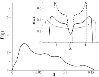
Figure 2: Main frame: Overlap probability distribution, $P(q)$, at zero temperature and $t=0.23$ in the VBG. The data are averaged over $16$ different realizations of the graph, with ${\cal N}=256$. The delta function in $q=0$ corresponds to the fraction of replicas which end up in the same state, and it is expected to disappear in the thermodynamic limit (e.g., for a system of ${\cal N}=128$ sites the delta peak in zero is approximately $1.5$ bigger than that for ${\cal N}=256$). Inset: Electron spectrum, $\rho(\lambda)$, at zero temperature in the different phases: Fermi liquid at $t=0.34$ (corresponding to the point marked by $\times$ in the phase diagram of Fig. 1, dotted line), Valence Bond Glass at $t=0.23$ (point marked by $\bullet$ in Fig. 1, continuous line) and Dimer phase at $t=0.16$ (point marked by $\blacksquare$ in Fig. 1, dashed line). The electron spectrum has been computed analytically in the uniform and in the dimer phase, and numerically in the VBG phase.

Valence Bond Glass— In order to study and prove the existence of the Valence Bond Glass phase we use Monte Carlo annealing simulations for the reasons explained previously. First, we check that our numerical procedure gives back the uniform (dimer) phase at high (low) enough temperature and hopping amplitude. In the intermediate region where both phases are unstable (e.g., at zero temperature for $0.218<t\leq 0.29$) we find that amorphous configurations of $\chi_{ij}$ correspond to the actual minima of the free energy. This is a glassy phase, which we call valence bond glass. This is not a spin glass since the average value of the spin is zero on each site of the lattice, $\langle\mathbf{S}_{i}\rangle=0$, as the $SU(N)$ symmetry is unbroken.
The valence bonds, $\chi_{ij}$, are real valued and their disordered profile is described by a nontrivial distribution, $P(\chi)$, as schematically depicted in the inset of Fig. 1. The electron spectrum is gapless in the VBG, although it exhibits a pseudo gap, as shown in the inset of Fig. 2, which becomes deeper and deeper as either the temperature or the hopping amplitude are decreased.
Interestingly enough, similarly to spin glasses [6], on any given graph different annealing procedures may lead to different configurations with the same free energy. One can measure the distributions of the overlaps between different states, defined as: $q_{ab}=\frac{2}{z{\cal N}}\sum_{\langle i,j\rangle}|\chi_{ij}^{a}-\chi_{ij}^{b}|$. According to this definition, $q_{ab}=0$ if the bosonic field has the same configuration in the two states, whereas $q_{ab}>0$ otherwise. As in spin glasses, one can define the overlap distribution $P(q)=\sum_{a,b}w_{a}w_{b}\delta(q-q_{a,b})$ where $w_{a}$ is the thermodynamic weight of the amorphous state $a$ [6]. The overlap distribution is apparently continuous. $P(q)$, averaged over $16$ different realizations of the graph is plotted in Fig. 2, at zero temperature and for $t=0.23$.
The transition from the uniform phase to the valence bond glass is continuous: the free energy of the two phases coincide within our numerical accuracy on the line $t_{s}(T)$ where the liquid phase becomes unstable. Close to the transition point, the distribution of the $\chi_{ij}$ is peaked around the value $\chi$ which characterizes the uniform phase, and it gets broader and broader as the temperature and/or the hopping amplitude are decreased. This transition shares many common features with the transition from the paramagnetic phase to the spin glass phase observed in mean field (classical) spin glasses such as, for instance, the Sherrington-Kirkpatrick model [6]: in both cases, one finds a continuous transition with a continuous distribution of the overlaps. As a consequence it is natural to investigate whether the VBG phase is marginally stable as the spin glass phase [6]. This means that the VBG phase is critical not only at the transition but in the whole region of the phase diagram where it exists. In order to do that we study whether the spatial correlations among valence bonds on different links of the lattice $\langle\chi_{ij}(\omega_{n})\,\chi_{kl}(\omega_{n})\rangle_{c}^{2}$ are long-ranged (as previously we focus on $\omega_{n}=0$ which is expected to give the main contribution). The inverse of the free energy Hessian matrix gives directly the dimer-dimer correlations. Instead of inverting this matrix, we follow a less computational demanding route using a kind of fluctuation-dissipation relation. The idea is to measure the response of the system, more precisely of the value of $\chi_{ij}$, to an external perturbation and relate it to the VBG susceptibility. The relevant perturbation for the present case is a local increase of the hopping amplitude on a given link of the graph, $t\to t+\delta t_{kl}$. Simple integrations by parts in the functional integral defining the partition function, Eq. (3), allow one to establish the following identity:

$$\chi_{\textrm{VBG}}=\frac{1}{z{\cal N}}\!\sum_{(ij)\neq(kl)}\!\!\left\langle\chi_{ij}^{0}\,\chi_{kl}^{0}\right\rangle_{c}^{2}=\frac{1}{z{\cal N}}\!\sum_{(ij)\neq(kl)}\!\left(\frac{\textrm{d}\langle\chi_{ij}^{0}\rangle}{\textrm{d}t_{kl}}\right)^{2}.$$ (18)

where $\chi_{ij}^{0}$ is a short-hand notation for $\chi_{ij}(\omega_{n}=0)$ and the subscript $c$ denotes the connected correlation function. We measured the response functions in the RHS of eq. (18). We found, as shown in Fig. 3, that the valence bond glass non-linear susceptibility, $\chi_{\textrm{VBG}}$, diverges as a power law both at fixed $t$ as the temperature is decreased ($\chi_{2}\sim(T-T_{s})^{-\gamma}$), and at fixed $T$ (included $T=0$) as the hopping is decreased ($\chi_{2}\sim(t-t_{s})^{-\gamma^{\prime}}$). The exponents have the mean field value $\gamma\simeq\gamma^{\prime}\simeq 1$. Furthermore we find that $\chi_{\textrm{VBG}}$ is infinite (meaning of the order of, and scaling as, $\cal N$) in all the VBG phase, hence, confirming the marginality of the VBG phase.
Differently from the transition from the liquid phase to the VBG, the transition from the dimer phase to the glassy one is discontinuous. It takes place at $t_{c}(T)$, where the free energies of the two phases coincide (at $T=0$ we have that $t_{c}\simeq 0.175$). The dimer phase becomes unstable only for larger values of $t$. Furthermore the non-linear susceptibility, $\chi_{\textrm{VBG}}$, stays finite approaching VBG from the dimer phase as it is expected for a first order transition.

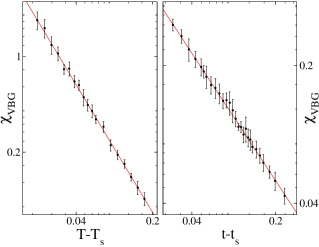
Figure 3: Valence bond non-linear susceptibility, $\chi_{\textrm{VBG}}$, as a function of $T-T_{s}$ at fixed $t=0.1$ (left panel) and as a function of $t-t_{s}$ at zero temperature (right panel). $\chi_{\textrm{VBG}}$ diverges as a power law as the transition to the VBG is approached. In both cases the exponent is compatible with $\gamma\sim 1$. The data are averaged over $8$ different realization of graphs with ${\cal N}=512$ sites.

In summary the Valence Bond Glass phase is characterized by an amorphous arrangement of dimers and absence of magnetic ordering. It has long-range critical dimer-dimer correlations in the whole VBG phase (not only at the transition). It has no gap in the electronic and spin density of states, although we observe a pseudo-gap. As a consequence it is related to, but quite different from, valence bond crystal and spin glass phases. We expect the VBG phase to be generically one of the possible low temperature phases arising from the interplay of strong quantum fluctuations and frustration. In the future it would be important to go beyond the simplifying framework we focused on. The role of $1/N$ corrections should be elucidated. Furthermore, it would be interesting to study different models, different (and more realistic) lattices and add some kind of local quenched disorder. The large $N$ approximation and the type of lattice we chose favor the glassy phase. In reality we expect that VBG will emerge as a true thermodynamic phase only in presence of some kind of quenched disorder (not much if there is already geometrical frustration). In this case the VBG phase will be in competition with the spin glass phase which in our treatment is excluded from the beginning because of the type of large $N$ limit we used. Another interesting route to follow is to study the effect of doping and the resulting properties of the VBG phase. This could be relevant for underdoped high $T_{c}$ superconducting materials. Although the VBG phase may not be a true thermodynamic stable phase it could nevertheless capture some kind of metastable slow and glassy dynamics which seems indeed to be present [20]. From a more fundamental and technical point of view obtaining a complete solution of our model (analytically or by numerical simulations) would be important to determine whether, as our results suggest, the VBG phase is completely analogous to the mean-field spin glass phase [6]. Finally, it is worth studying the effect of magneto-elastic couplings. Because of the marginal stability of the VBG phase they could play a very important role. We expect as experimental signature of the valence bond glass phase spatially heterogeneous NMR signals. Furthermore, approaching the (continuous) transition toward the VBG phase, the VBG susceptibility diverges and this could lead to anomalous (even divergent) non-linear pressure responses. Finally, we point out that preliminary results on modified random lattices (e.g., random regular graphs where each site is replaced by square plaquettes) show that also glassy flux phases [10] might appear. These are characterized by amorphous circulating micro-currents.

1 Appendix

Here we describe in detail the Monte Carlo annealing simulations we used. We pick up a link $(ij)$ at random out of the $z{\cal N}/2$ total links and try to change either the real or the imaginary part of $\chi_{ij}$ by a random amount $\delta\in(-\delta_{max},\delta_{max})$ with probability $1/2$ respectively. Then we compute the new free energy, according to Eq. (8). Since $F(\chi)$ contains a non-local term, at each step we have to diagonalize the matrix $t\mathbb{C}+\hat{\chi}$ and compute all its eigenvalues, which takes a computational time proportional to ${\cal N}^{2}$. The move is accepted with probability $p=\textrm{min}\left\{1,\exp[-\Delta F/T_{aux}]\right\}$. The value of $\delta_{max}$ is self-adapted during the simulation in such a way that the average acceptance rate of the moves is $0.3$. We have checked that several different values of the chosen acceptance rate lead to the same results. The auxiliary temperature is decreased at constant rate down to very low temperature, starting from $T_{aux}=0.5$. Most of the results presented here have been obtained with a rate $\Gamma=\dot{T}_{aux}/T_{aux}=1.3\cdot 10^{-3}$ (where each MC step consists of $z{\cal N}$ total attempts). We have verified that slower cooling rates down to $\Gamma\sim 5\cdot 10^{-5}$ do not change the results. Some MC steps are finally performed at $T_{aux}=0$.

References

- [1] P.W. Anderson, Mat. Res. Bull. 8 153, (1973).
- [2] P.A. Lee, Rep. Prog. Phys. 71, 012501 (2008).
- [3] P.W. Anderson, Science 235, 1196 (1987).
- [4] G. Misguich, C. Lhuillier, in “Frustrated spin systems”, H. T. Diep editor, World-Scientific (2005).
- [5] M. Tamura, A. Nakao and R. Kato, J. Phys. Soc. Japan 75 093701 (2006).
- [6] M. Mézard, G. Parisi, and M.A. Virasoro, Spin-glass Theory and Beyond, vol. 9 of Lecture notes in Physics, World Scientific, Singapore, 1987. Binder and A. P. Young, Rev. Mod. Phys. 58, 801 (1986).
- [7] Dupuis et al., J. Appl. Phys. 91, 8384 (2002); Limot et al. Phys. Rev. B 65, 144447 (2002); S.-W. Han, J.S. Gardner, and C.H. Booth, Phys. Rev. B 69, 024416 (2004).
- [8] C. Henley, Can. J. Phys. 79 1307 (2001).
- [9] Ladieu et al., J. Phys.: C 16, S735-S741 (2004).
- [10] J.B. Martson and I. Affleck, Phys. Rev. B 39, 11538 (1989).
- [11] R. Baxter, Exactly Solved Models in Statistical Mechanics, (Academic Press, London, 1982).
- [12] M. Mézard and G. Parisi, Eur. Phys. J. B 20, 217 (2001).
- [13] G. Biroli and M. Mézard, Phys. Rev. Lett. 88, 025501 (2002).
- [14] D.S. Rokhsar, Phys. Rev. B 42, 2526 (1990).
- [15] A. Georges et al., Rev. Mod. Phys. 68, 1 (1996).
- [16] C. Laumann, A. Scardicchio, and S.L. Sondhi, arxiv:0706.4391 (2007).
- [17] D.J. Thouless, P.W. Anderson and R.G. Palmer, Phil. Mag. 35, 593 (1977).
- [18] See e.g. A.J. Bray and G.J. Rodgers, Phys. Rev. B 38, 11461 (1988).
- [19] L. Zdeborovà, M. Mézard, J. Stat. Mech. P05003 (2006).
- [20] Y. Kohsaka et al., Science 315, 1380 (2007).