Relativistic quasiparticle time blocking approximation. Dipole response of open-shell nuclei

Abstract

The self-consistent Relativistic Quasiparticle Random Phase Approximation (RQRPA) is extended by the quasiparticle-phonon coupling (QPC) model using the Quasiparticle Time Blocking Approximation (QTBA). The method is formulated in terms of the Bethe-Salpeter equation (BSE) in the two-quasiparticle space with an energy-dependent two-quasiparticle residual interaction. This equation is solved either in the basis of Dirac states forming the self-consistent solution of the ground state or in the momentum representation. Pairing correlations are treated within the Bardeen-Cooper-Schrieffer (BCS) model with a monopole-monopole interaction. The same NL3 set of the coupling constants generates the Dirac-Hartree-BCS single-quasiparticle spectrum, the static part of the residual two-quasiparticle interaction and the quasiparticle-phonon coupling amplitudes. A quantitative description of electric dipole excitations in the chain of tin isotopes ($Z=50$) with the mass numbers $A=$ 100, 106, 114, 116, 120, and 130 and in the chain of isotones with ($N=50$) ⁸⁸Sr, ⁹⁰Zr, ⁹²Mo is performed within this framework.

The RQRPA extended by the coupling to collective vibrations generates spectra with a multitude of $2q\otimes phonon$ (two quasiparticles plus phonon) states providing a noticeable fragmentation of the giant dipole resonance as well as of the soft dipole mode (pygmy resonance) in the nuclei under investigation. The results obtained for the photo absorption cross sections and for the integrated contributions of the low-lying strength to the calculated dipole spectra agree very well with the available experimental data.

I Introduction

Theoretical approaches based on Covariant Density Functional Theory (CDFT) remain undoubtedly among the most successful microscopic descriptions of nuclear structure. The CDFT approaches are derived from a Lorentz invariant density functional which connects in a consistent way the spin and spatial degrees of freedom in the nucleus. Therefore, it needs only a relatively small number of parameters which are adjusted to reproduce a set of bulk properties of spherical closed-shell nuclei Rin.96 ; VALR.05 and it is valid over the entire periodic table. Over the years, Relativistic Mean-Field (RMF) models based on the CDFT have been successfully applied to describe ground state properties of finite spherical and deformed nuclei over the entire nuclear chart GRT.90 from light nuclei LVR.04a to super-heavy elements LSRG.96 ; BBM.04 , from the neutron drip line where halo phenomena are observed MR.96 , to the proton drip line LVR.04 with nuclei unstable against the emission of protons  LVR.99 . The relativistic cranking approximation has been developed to calculate rotational bands KR.89 ; ARK.00 . For a description of nuclear excited states, the Relativistic Random Phase Approximation (RRPA) RMG.01 and the quasiparticle RRPA (RQRPA) PRN.03 have been formulated as the small amplitude limit of the time-dependent RMF models. These models have provided a very good description for the positions of giant resonances and a theoretical interpretation of the low-lying dipole PRN.03 and quadrupole Ans.05 ; AR.06 excitations. Proton-neutron versions of the RRPA and the RQRPA have been developed and successfully applied to the description of spin/isospin excitations as the Isobaric Analog Resonance (IAR) or the Gamow-Teller Resonance (GTR) PNV.04 .

Recently, several attempts have been made to extend the RMF and RRPA formalism beyond the mean field approach, first of all, to solve the well known problem of the RMF single-particle level density in the vicinity of the Fermi surface which is too low because of the too small effective mass. The energy dependence of the single-nucleon self-energy was emulated in a phenomenological way VNR.02 and microscopically by coupling the single particle configurations to low-lying surface vibration LR.06 . This provided a considerable improvement for the description of the single-particle spectra. An addition, the quadrupole motion has been studied within the relativistic Generator Coordinate Method (GCM)  NVR.06a ; NVR.06b .

In Refs. LRT.07 ; LRV.07 , we have extended the relativistic RPA by introducing a coupling to collective vibrations using the techniques developed and realized long ago for non-relativistic approaches in terms of the Green’s function formalism Tse.89a ; Tse.89 ; KTT.97 ; KST.04 . An induced additional interaction between single-particle and vibrational excitations provided a strong fragmentation of the pure RRPA states causing the spreading width of giant resonances and the redistribution of the pygmy strength to lower energies. This method does not include pairing correlations and therefore it is restricted essentially to the few nuclei with doubly closed shells in the nuclear chart.

In the present work we consider systems with pairing correlations. Again, we are guided by ideas of the quasiparticle time-blocking approximation (QTBA) developed and applied for non-relativistic systems in Refs. Tse.07 and LT.07 , which takes into account quasiparticle-phonon coupling (QPC) and pairing correlations on an equal footing. However, our approach is based on CDFT and formulated in terms of relativistic Green’s functions of the Dirac-Hartree-Bogoliubov (DHB) or the Dirac-Hartree-BCS (DHBCS) equations. Similar, but in details different, approaches developed earlier within a non-relativistic formalism can be found in Refs. Sol.92 ; BP.99 ; CB.01 .

The main assumption of the quasiparticle-phonon coupling model BM.75 is that the two types of elementary excitations – two-quasiparticle and vibrational modes – are coupled in such a way that configurations of $2q\otimes phonon$ type with low-lying phonons strongly compete with simple $2q$ configurations close in energy or, in other words, that quasiparticles can emit and absorb phonons with rather high probabilities. Obviously, these processes should affect both the ground and excited states and therefore, the corresponding amplitudes should be taken into account both in the single-nucleon self-energy and in the effective interaction in the nuclear interior.

In order to describe excited states in nuclei, we extend covariant density functional theory by coupling the quasiparticles to low-lying vibrations in a consistent way using effective interactions derived from the same Lagrangian without additional phenomenological parameters. First of all, we use the well-known quasiparticle formalism, where, in terms of second quantization, nucleon creation and annihilation operators become components of a two-component operator mixing a creation and annihilation of a particle into a single quasiparticle. This leads to the fact, that for systems with pairing correlations all quantum operators become tensors in the two-dimensional quasiparticle space. In particular, the relativistic energy functional is expressed in terms of the relativistic extension of the Valatin density matrix Val.61 of double dimension containing the normal as well as the abnormal densities. As discussed in detail in Refs. Kuc.89 ; KuR.91 ; SRRi.02 ; SR.02 pairing correlations can be considered in a very good approximation as a non-relativistic effect and therefore the full density functional is a sum of the relativistic energy functional depending on the normal density and derived from the underlying Lagrangian and a non-relativistic pairing energy $E_{pair}$, depending on the abnormal density. The equations of motion are the self-consistent Relativistic Hartree Bogoliubov (RHB) equations. They are derived from this general functional by variation with respect to the Valatin density matrix. They are solved numerically and the self-consistent fields obtained in this way, which do not depend on the energy, form the static part of the nucleon self-energy. This static part determines the nuclear ground state in the mean field approximation.

The static effective interaction used in conventional QRPA approximation is derived as the second derivative of the same energy functional and therefore it contains no additional parameters. It enables us to go a step further and to compute amplitudes, or vertices, which describe the emission or absorption of phonons by quasiparticles within the relativistic framework. These amplitudes form the essential ingredient for the following considerations. They determine an additive energy-dependent and non-local term in the self-energy of the single-quasiparticle equation of motion and, consequently, an induced effective interaction between the quasiparticles. Both of these quantities have an influence on the $ph$- as well as on the $pp$-channel.

For the calculation of the response of a nucleus in an external field we use the Bethe-Salpeter equation. It contains both the static and the induced effective interactions and it is formulated in the doubled two-quasiparticle basis of the Dirac-Hartree-Bogoliubov eigenstates. This Bethe-Salpether equation describes the quasiparticle-phonon coupling and pairing correlations on the equal footing. It is solved using the quasiparticle time blocking approximation (QTBA) developed in Ref. Tse.07 , which allows the truncation to $2q\otimes phonon$ configurations and guarantees that the solution is positive defined. We also use the subtraction procedure introduced and justified in the Ref. Tse.07 . As in the case without pairing it avoids double counting of the QPC. At zero energy, i.e. at the ground state, particle vibrational coupling should have no influence, because the correlations induced by QPC in the ground state have already been taken into account in the RHB description through the parameters of the energy functional initially fitted to reproduce experimental data, such as nuclear binding energies and radii. Therefore, the relativistic mean field contains effectively all the correlations in the static approximation. The energy dependence of the self energy influences only excitations at finite energy in the nucleus.

In the present work we develop the Relativistic Quasiparticle Time Blocking Approximation (RQTBA) and apply it for the description of electric dipole excitations in even-even spherical open-shell nuclei, such as the tin ($Z=50$) isotopes ^{100,106,114,116,120,130}Sn and the ($N=50$) isotones ⁸⁸Sr, ⁹⁰Zr, ⁹²Mo. The RQTBA method, whose physical content is an extension of the RQRPA by a coupling to low-lying collective vibrations, provides spectra enriched with the $2q\otimes phonon$ states. They cause a strong redistribution of the RQRPA strength. As a result, we obtain an additional broadening of the giant dipole resonance and a spreading of the soft dipole mode (pygmy resonance) to lower energies in the nuclei under investigation.

The paper is organized as follows. In Section II we formulate basic relations of our approach in a rather general form. In Section III we give a more detailed formalism for spherical nuclei in the form adopted for numerical calculations. Section IV is devoted to the description of some numerical details and to the presentation of our results for even-even semi-magic nuclei. Finally, Section V contains conclusions and an outlook.

II General formalism

II.1 Basic relations of the covariant density functional theory for nuclei with pairing

In this subsection we recall the general formalism of covariant density functional theory with pairing, introduce notations and determine conventions used later on.

In open-shell nuclei, pairing correlations play an essential role and have to be incorporated consistently in a description of the ground state as well as of excited states including many-body dynamics. Considering $pp$-correlations in addition to the usual $ph$-interaction, existing in normal systems, one has to provide a unified description of both $pp$- and $ph$-channels.

In contrast to Hartree- or Hartree-Fock theory, where $pp$-correlations are neglected, and where the building blocks of excitations (the quasiparticles in the sense of Landau) are either nucleons in levels above the Fermi surface (particles) or missing nucleons in levels below the Fermi surface (holes), we have now quasiparticles in the sense of Bogoliubov which are described by a combination of creation and annihilation operators. This fact can be expressed in a standard way by introducing the following two-component operator, which is a generalization of the usual particle annihilation operator:

$$\Psi(1)=\left(\begin{array}[c]{c}a(1)\\ a^{\dagger}(1)\end{array}\right).$$ (1)

Here $a(1)=e^{iHt_{1}}a_{k_{1}}e^{-iHt_{1}}$ is a nucleon annihilation operator in the Heisenberg picture and the quantum numbers $k_{1}$ represent an arbitrary basis, $1=\{k_{1},t_{1}\}$. In order to keep the notation simple we use in the following $1=\{\mbox{\boldmath$r$}_{1},t_{1}\}$ and omit spin and isospin indices.

Let us introduce the chronologically ordered product of the operator $\Psi(1)$ in Eq. (1) and its Hermitian conjugated operator $\Psi^{\dagger}(2)$, averaged over the ground state $|\Phi_{0}\rangle$ of the system which will be concretized below. This tensor of rank 2

$$G(1,2)=-i\langle\Phi_{0}|T\Psi(1)\Psi^{\dagger}(2)|\Phi_{0}\rangle\ \$$ (2)

is the generalized Green’s function which can be expressed through a 2$\times$2 matrix:

$$G(1,2) =-i\theta(t_{1}-t_{2})\langle\Phi_{0}|\left(\begin{array}[c]{cc}a(1)a^{\dagger}(2)&a(1)a(2)\\ a^{\dagger}(1)a^{\dagger}(2)&a^{\dagger}(1)a(2)\end{array}\right)|\Phi_{0}\rangle$$ (5)

$$+i\theta(t_{2}-t_{1})\langle\Phi_{0}|\left(\begin{array}[c]{cc}a^{\dagger}(2)a(1)&a(2)a(1)\\ a^{\dagger}(2)a^{\dagger}(1)&a(2)a^{\dagger}(1)\end{array}\right)|\Phi_{0}\rangle.$$ (8)

Similar definitions for the Green’s function in non-relativistic superfluid systems have been used in Refs. Gor.58 ; BW.63 ; Tse.07 ; LT.07 . Notice that we define the definition of Green’s functions here in the way of non-relativistic many-body theory, which differs form the conventional definition $\langle T\Psi\bar{\Psi}\rangle$ adopted in relativistic field theories by the replacement of $\bar{\Psi}$ by $\Psi^{\dagger}$, i.e. by a Dirac matrix $\beta=\gamma_{0}$. This notation is more convenient for our analysis and the matrix $\beta$ needed for Lorentz invariance is included in the vertices. Therefore the generalized density matrix is obtained as a limit

$$\mathcal{R}(\mbox{\boldmath$r$}_{1},\mbox{\boldmath$r$}_{2},t_{1})=-i\lim\limits_{t_{2}\rightarrow t_{1}+0}G(1,2)$$ (9)

from the second term of Eq. (8), and, in the notation of Valatin Val.61 , it can be expressed as a matrix of doubled dimension containing as components the normal density ${{\rho}}$ and the abnormal density ${{\varkappa}}$, the so called pairing tensor:

$$\mathcal{R}(\mbox{\boldmath$r$}_{1},\mbox{\boldmath$r$}_{2},t)=\left(\begin{array}[c]{cc}\rho(\mbox{\boldmath$r$}_{1},\mbox{\boldmath$r$}_{2},t)&\varkappa(\mbox{\boldmath$r$}_{1},\mbox{\boldmath$r$}_{2},t)\\ -\varkappa^{\ast}(\mbox{\boldmath$r$}_{1},\mbox{\boldmath$r$}_{2},t)&\delta(\mbox{\boldmath$r$}_{1}-\mbox{\boldmath$r$}_{2})-\rho^{\ast}(\mbox{\boldmath$r$}_{1},\mbox{\boldmath$r$}_{2},t)\end{array}\right).$$ (10)

These densities play a key role in the description of a superfluid many-body system.

In covariant density functional theory for normal systems the ground state of the nucleus is a Slater determinant describing nucleons, which move independently in meson fields $\phi_{m}$ characterized by their quantum numbers for spin, parity and isospin. In the present investigation we use the concept of conventional relativistic mean field theory and include the $\sigma$, $\omega$, $\rho$-meson fields and the electromagnetic field as the minimal set of fields providing a rather good quantitative description of bulk and single-particle properties in the nucleus Wal.74 ; SW.86 ; Rin.96 . This means that the index $m$ runs over the different types of fields $m=\{\sigma,\omega,\rho,A\}$. The summation over $m$ implies in particular scalar products in Minkowski space for the vector fields and in isospace for the $\rho$-field. In order to obtain a Lorentz invariant theory, these classical fields $\phi_{m}=\{\sigma,\omega^{\mu},{\vec{\rho}}^{\ \mu},A^{\mu}\}$ are generated in a self-consistent way by the exchange of virtual particles, called mesons, and the photon.

Finally the energy depends in the case without pairing correlations on the normal density matrix ${\rho}$ and the various fields $\phi_{m}$:

$$E_{RMF}[{{\rho}},\phi]=\text{Tr}[({\mbox{\boldmath$\alpha$}}\mathbf{p}+\beta m){{\rho}}]+\sum\limits_{m}\Bigl{\{}\text{Tr}[(\beta\Gamma_{m}\phi_{m}){{\rho}}]\pm\int\Bigl{[}\frac{1}{2}(\mbox{\boldmath$\nabla$}\phi_{m})^{2}+U_{m}(\phi)\Bigr{]}d^{3}r\Bigr{\}}$$ (11)

Here we have neglected retardation effects, i.e. time-derivatives of the fields $\phi_{m}$. The plus sign in Eq. (11) holds for scalar fields and the minus sign for vector fields. The trace operation implies a sum over Dirac indices and an integral in coordinate space. $\alpha$ and $\beta$ are Dirac matrices and the vertices $\Gamma_{m}$ are given by

$$\Gamma_{\sigma}=g_{\sigma},\ \ \ \ \Gamma_{\omega}^{\mu}=g_{\omega}\gamma^{\mu},\ \ \ \ {\vec{\Gamma}}_{\rho}^{\ \mu}=g_{\rho}{\vec{\tau}}\gamma^{\mu},\ \ \ \ \Gamma_{e}^{\mu}=e\frac{(1-\tau_{3})}{2}\gamma^{\mu}$$ (12)

with the corresponding coupling constants $g_{m}$ for the various meson fields and for the electromagnetic field.

The quantities $U_{m}(\phi)$ are, in the case of a linear meson couplings, given by the term

$$U_{m}(\phi)=\frac{1}{2}m_{m}^{2}\phi_{m}^{2}$$ (13)

containing the meson masses $m_{m}$. For non-linear meson couplings, as for instance for the $\sigma$-meson in the parameter set NL3 we have, as proposed in Ref. BB.77 :

$$U(\sigma)=\frac{1}{2}m_{\sigma}^{2}\sigma^{2}+\frac{g_{2}}{3}\sigma^{3}+\frac{g_{3}}{4}\sigma^{4}\;.$$ (14)

with two additional coupling constants $g_{2}$ and $g_{3}$.

In superfluid covariant density functional theory the energy is a functional of the Valatin density $\mathcal{{R}}$ and the fields $\phi_{m}$. Therefore Relativistic Hartree-Bogoliubov (RHB) theory can be derived from an energy functional which depends on the normal density ${{\rho}}$ and the abnormal density ${{\varkappa}}$ as well as on the meson and Coulomb fields $\phi_{m}$. We use here a density functional of the form

$$E_{RHB}[{{\rho}},{{\varkappa}},{{\varkappa}}^{\ast},\phi]=E_{RMF}[{{\rho}},\phi]+E_{pair}[{{\varkappa},{\varkappa}}^{\ast}]$$ (15)

where the pairing energy is expressed by an effective interaction ${\tilde{V}}^{pp}$ in the $pp$-channel:

$$E_{pair}[{{\varkappa},{\varkappa}}^{\ast}]=\frac{1}{4}Tr[{{\varkappa}}^{\ast}{\tilde{V}}^{pp}{{\varkappa}}].$$ (16)

Here and in the following a tilde sign is used to express the static character of a quantity, i.e. the fact that it does not depend on the energy. Of course, in Eq. (15) we could also use density dependent pairing forces with $E_{pair}=E_{pair}[{\rho},{{\varkappa}}]$ as it is done for instance in Refs. FTT.00 ; BE.91 . However, in the present investigation we do not consider this possibility. The effective interaction $\tilde{V}^{pp}$ in the particle-particle channel is supposed to be independent on the interaction in the particle-hole channel (see, e.g., Ref. PRN.03 ) mediated by the mesons and the electromagnetic fields determined above. Generally, the form of $\tilde{V}^{pp}$ is restricted only by the conditions of the relativistic invariance of $E_{pair}$ with respect to the transformations of the abnormal densities (see Ref. CG.99 ). In this section, we consider the general form of $\tilde{V}^{pp}$ as a non-local function in coordinate representation. In all the applications discussed in Section III we use for $\tilde{V}^{pp}$ a simple monopole-monopole interaction.

The classical variational principle applied to the energy functional of Eq. (15)

$$\delta\int\limits_{t_{1}}^{t_{2}}\Bigl{(}\langle\Phi_{0}|i\partial_{t}|\Phi_{0}\rangle-E_{RHB}[{{\rho}},{{\varkappa}},{{\varkappa}}^{\ast},\phi]\Bigr{)}dt=0$$ (17)

leads to the equation of motion for the generalized density matrix $\mathcal{R}$:

$$i\partial_{t}{{\mathcal{R}}}=[{{\mathcal{H}}}_{RHB}({{\mathcal{R}}}),{{\mathcal{R}}}]$$ (18)

with the RHB Hamiltonian

$${{\mathcal{H}}}_{RHB}=2\frac{\delta E_{RHB}}{\delta\mathcal{R}}=\left(\begin{array}[c]{cc}h^{\mathcal{D}}-m-\lambda&\Delta\\ -\Delta^{\ast}&-h^{\mathcal{D}\ast}+m+\lambda\end{array}\right),$$ (19)

where $\lambda$ is the chemical potential (conted from the continuum limit). In the static case we find

$$[{{\mathcal{H}}}_{RHB}({{\mathcal{R}}}),{{\mathcal{R}}}]=0.$$ (20)

Because of time reversal invariance the currents vanish and we obtain the single nucleon Dirac Hamiltonian

$$h^{\mathcal{D}}={\mbox{\boldmath$\alpha$}}\mathbf{p}+\beta(m+{\tilde{\Sigma}})\ \ \$$ (21)

with the RMF self-energy

$${\tilde{\Sigma}}(\mbox{\boldmath$r$})=\sum\limits_{m}\Gamma_{m}\phi_{m}(\mbox{\boldmath$r$})$$ (22)

The pairing field $\Delta$ reads in this case:

$$\Delta(\mbox{\boldmath$r$},\mbox{\boldmath$r$}^{\prime})=\frac{1}{2}\int d{\mbox{\boldmath$r$}}^{\prime\prime}d{\mbox{\boldmath$r$}}^{\prime\prime\prime}{\tilde{V}}^{pp}(\mbox{\boldmath$r$},\mbox{\boldmath$r$}^{\prime},\mbox{\boldmath$r$}^{\prime\prime},\mbox{\boldmath$r$}^{\prime\prime\prime})\varkappa(\mbox{\boldmath$r$}^{\prime\prime},\mbox{\boldmath$r$}^{\prime\prime\prime}).$$ (23)

Eq. (20) leads to the relativistic Hartree-Bogoliubov equations KuR.91

$$\mathcal{H}_{RHB}|\psi_{k}^{\eta}\rangle=\eta E_{k}|\psi_{k}^{\eta}\rangle,\ \ \ \ \eta=\pm 1$$ (24)

where $|\psi_{k}^{\eta}\rangle$ are the eigenfunctions corresponding to eigenvalues $\eta E_{k}$. They are the 8-dimensional Bogoliubov-Dirac spinors of the following form

$$|\psi_{k}^{+}(\mbox{\boldmath$r$})\rangle=\left(\begin{array}[c]{c}U_{k}(\mbox{\boldmath$r$})\\ V_{k}(\mbox{\boldmath$r$})\end{array}\right),\ \ \ \ |\psi_{k}^{-}(\mbox{\boldmath$r$})\rangle=\left(\begin{array}[c]{c}V_{k}^{\ast}(\mbox{\boldmath$r$})\\ U_{k}^{\ast}(\mbox{\boldmath$r$})\end{array}\right).$$ (25)

Note that the index $k$ labels here and in the following quasiparticles in contrast to the index $k_{1}$ used after Eq. (1) for the particle basis. In the following we call this quasiparticle basis the Dirac-Hartree-Bogoliubov (DHB) basis.

The generalized density matrix is obtained as follows:

$$\mathcal{R}(\mbox{\boldmath$r$},\mbox{\boldmath$r$}^{\prime})=\sum\limits_{k}|\psi_{k}^{-}(\mbox{\boldmath$r$})\rangle\langle\psi_{k}^{-}(\mbox{\boldmath$r$}^{\prime})|,$$ (26)

where the summation is performed only over the states having large upper components of the Dirac spinors (i.e. large functions $f_{(k)}(r)$ in Eq. (68) below). This restriction corresponds to the so-called no-sea approximation (see Ref. SR.02 ).

The behavior of the meson and Coulomb fields is derived from the energy functional (15) by variation with respect to the fields $\phi_{m}$. We obtain Klein-Gordon equations. In the static case they have the form

$$-\Delta\phi_{m}(\mbox{\boldmath$r$})+U^{\prime}(\phi_{m}(\mbox{\boldmath$r$}))=\mp\sum\limits_{k}V_{k}^{\intercal}(\mbox{\boldmath$r$})\beta\Gamma_{m}V_{k}^{\ast}(\mbox{\boldmath$r$}),$$ (27)

Eq. (27) determines the potentials entering the single-nucleon Dirac Hamiltonian (21) and is solved self-consistently together with Eq. (24). The system of Eqs. (24) and (27) determine the ground state of an open-shell nucleus in the relativistic Hartree-Bogoliubov approach.

II.2 Quasiparticle-vibration coupling as a model for an energy dependence of the single-quasiparticle self-energy

The single quasiparticle equation of motion (24) determines the behavior of a nucleon with a static self energy. To include dynamics, i.e. a more realistic time dependence in the self energy one has to extend the energy functional by an appropriate term leading to a self-energy (22) with time dependence. In the present work we use for this purpose the successful but relatively simple particle-vibration coupling model introduced in Refs. BM.75 ; AGD.63 . Following the general logic of this model, we consider the total single-nucleon self-energy for the Green’s function defined in Eq. (2) as a sum of the RHB self-energy and an energy-dependent non-local term in the doubled space:

$${{\Sigma}}(\mbox{\boldmath$r$},\mbox{\boldmath$r$}^{\prime};\varepsilon)={{\tilde{\Sigma}}}(\mbox{\boldmath$r$},\mbox{\boldmath$r$}^{\prime})+{{\Sigma}^{(e)}}(\mbox{\boldmath$r$},\mbox{\boldmath$r$}^{\prime};\varepsilon)$$ (28)

with

$${{\tilde{\Sigma}}}(\mbox{\boldmath$r$},\mbox{\boldmath$r$}^{\prime})=\left(\begin{array}[c]{cc}\beta{\tilde{\Sigma}}(\mbox{\boldmath$r$})\delta(\mbox{\boldmath$r$}-\mbox{\boldmath$r$}^{\prime})&\Delta(\mbox{\boldmath$r$},\mbox{\boldmath$r$}^{\prime})\\ -\Delta^{\ast}(\mbox{\boldmath$r$},\mbox{\boldmath$r$}^{\prime})&-\beta{\tilde{\Sigma}}^{\ast}(\mbox{\boldmath$r$})\delta(\mbox{\boldmath$r$}-\mbox{\boldmath$r$}^{\prime})\end{array}\right).$$ (29)

The energy-dependent operator ${{\Sigma}^{(e)}}(\mbox{\boldmath$r$},\mbox{\boldmath$r$}^{\prime};\varepsilon)$ will be determined below (the upper index $e$ in this quantity indicates the energy dependence). The Dyson equation for the single-quasiparticle Green’s function (2) in the doubled space has the following form:

$$(\varepsilon-\mathcal{H}_{RHB}-\Sigma^{(e)}(\varepsilon))G(\varepsilon)=1$$ (30)

To study the influence of the energy-dependent part of the self-energy on the single-quasiparticle energies, it is convenient to formulate Eq. (30) in the basis of the eight-component Dirac spinors $|\psi_{k}^{\eta}\rangle$ which diagonalize the static RHB-Hamiltonian $\mathcal{H}_{RHB}$ in Eq. (24):

$$\sum\limits_{\eta=\pm 1}\sum\limits_{k}\Bigl{(}(\varepsilon-\eta_{1}E_{k_{1}})\delta_{\eta_{1}\eta}\delta_{k_{1}k}-\Sigma_{k_{1}k}^{(e)\eta_{1}\eta}(\varepsilon)\Bigr{)}G_{kk_{2}}^{\eta\eta_{2}}(\varepsilon)=\delta_{\eta_{1}\eta_{2}}\delta_{k_{1}k_{2}},$$ (31)

where

$$\Sigma_{k_{1}k_{2}}^{(e)\eta_{1}\eta_{2}}(\varepsilon)=\int d^{3}rd^{3}{r}^{\prime}~{}\langle{\psi}_{k_{1}}^{\eta_{1}}(\mbox{\boldmath$r$})|{{\Sigma}}^{(e)}({\mbox{\boldmath$r$}},{\mbox{\boldmath$r$}^{\prime}};\varepsilon)|\psi_{k_{2}}^{\eta_{2}}({\mbox{\boldmath$r$}^{\prime}})\rangle,$$ (32)

$$G_{k_{1}k_{2}}^{\eta_{1}\eta_{2}}(\varepsilon)=\int d^{3}rd^{3}{r}^{\prime}~{}\langle{\psi}_{k_{1}}^{\eta_{1}}(\mbox{\boldmath$r$})|\,{{G}}({\mbox{\boldmath$r$}},{\mbox{\boldmath$r$}^{\prime}};\varepsilon)|\psi_{k_{2}}^{\eta_{2}}({\mbox{\boldmath$r$}^{\prime}})\rangle.$$ (33)

In this basis the single-quasiparticle Green’s function ${\tilde{G}}$ of the static mean field has the following simple diagonal form:

$${\tilde{G}}_{k_{1}k_{2}}^{\eta_{1}\eta_{2}}(\varepsilon)=\delta_{k_{1}k_{2}}\delta_{\eta_{1}\eta_{2}}{\tilde{G}}_{k_{1}}^{\eta_{1}}(\varepsilon),\ \ \ \ \ {\tilde{G}}_{k_{1}}^{\eta_{1}}(\varepsilon)=\frac{1}{\varepsilon-\eta_{1}E_{k_{1}}+i\eta_{1}\delta},\ \ \ \ \ \ \delta\rightarrow+0.$$ (34)

As in Refs. LR.06 ; LRT.07 , we use the particle-phonon coupling model for the energy-dependent part of the self-energy $\Sigma^{(e)}$. In the basis of the spinors $|\psi_{k}^{\eta}\rangle$ of Eq. (25), called in the following Dirac basis, its matrix elements are given by:

$$\Sigma_{k_{1}k_{2}}^{(e)\eta_{1}\eta_{2}}(\varepsilon)=\sum\limits_{\eta=\pm 1}\sum\limits_{\eta_{\mu}=\pm 1}\sum\limits_{k,\mu}\frac{\delta_{\eta_{\mu},\eta_{3}}{\gamma}_{\mu;k_{1}k}^{\eta_{\mu};\eta_{1}\eta}\ {\gamma}_{\mu;k_{2}k}^{\eta_{\mu};\eta_{2}\eta\ast}}{\varepsilon-\eta E_{k}-\eta_{\mu}(\Omega_{\mu}-i\delta)},\ \ \ \ \delta\rightarrow+0.$$ (35)

The index $k_{3}$ formally runs over all single-quasiparticle states in the DHB basis including antiparticle states with negative energies. In the doubled quasiparticle space we can no longer distinguish occupied and unoccupied states considering that all the orbits are partially occupied. But in practical calculations, it is assumed that there are no pairing correlations in the Dirac sea SR.02 and the orbits with negative energies are treated in the no-sea approximation. As it has been shown in calculations for nuclei with closed shells in Ref. LR.06 , the numerical contribution of the diagrams with intermediate states $k$ with negative energy is very small due to the large energy denominators in the corresponding terms of the self-energy (35). The index $\mu$ in Eq. (35) labels the set of phonons taken into account. $\Omega_{\mu}$ are their frequencies and $\eta_{\mu}=\pm 1$ labels forward and backward going diagrams in Eq. (35). The vertices ${\gamma}_{\mu;k_{1}k_{2}}^{\eta_{\mu};\eta_{1}\eta_{2}}$ determine the coupling of the quasiparticles, to the collective state $\mu$:

$${\gamma}_{\mu;k_{1}k_{2}}^{\eta_{\mu};\eta_{1}\eta_{2}}=\delta_{\eta_{\mu},+1}{\gamma}_{\mu;k_{1}k_{2}}^{\eta_{1}\eta_{2}}+\delta_{\eta_{\mu},-1}{\gamma}_{\mu;k_{2}k_{1}}^{\eta_{2}\eta_{1}\ast},$$ (36)

In the conventional version of the particle-vibrational coupling model the phonon vertices $\gamma_{\mu}$ are derived from the corresponding transition densities $\mathcal{R}_{\mu}$ and the static effective interaction:

$$\gamma_{\mu;k_{1}k_{2}}^{\eta_{1}\eta_{2}}=\sum\limits_{k_{3}k_{4}}\sum\limits_{\eta_{3}\eta_{4}}\tilde{V}_{k_{1}k_{4},k_{2}k_{3}}^{\eta_{1}\eta_{4},\eta_{2}\eta_{3}}\mathcal{R}_{\mu;k_{3}k_{4}}^{\eta_{3}\eta_{4}},$$ (37)

where $\tilde{V}_{k_{1}k_{4},k_{2}k_{3}}^{\eta_{1}\eta_{4},\eta_{2}\eta_{3}}$ denotes a relativistic matrix element of the static residual interaction in the doubled space. It is obtained as a functional derivative of the relativistic mean-field self-energy ${{\tilde{\Sigma}}}$ with respect to the relativistic generalized density matrix ${\mathcal{R}}$:

$${\tilde{V}}_{k_{1}k_{4},k_{2}k_{3}}^{\eta_{1}\eta_{4},\eta_{2}\eta_{3}}=\frac{\ \delta{\tilde{\Sigma}}_{k_{4}k_{3}}^{\eta_{4}\eta_{3}}\ }{\ \delta\mathcal{R}_{k_{2}k_{1}}^{\eta_{2}\eta_{1}}\ }.$$ (38)

The transition densities $\mathcal{R}_{\mu}$ are defined by the time dependence of the generalized density (10)

$$\mathcal{R}(t)=\mathcal{R}_{0}+{\displaystyle\sum\limits_{\mu}}(\mathcal{R}_{\mu}e^{i\Omega_{\mu}t}+\text{h.c.)}$$ (39)

describing the oscillating system. We use the linearized version of the model which assumes that the transition densities $\mathcal{R}_{\mu}$ are not influenced by the particle-phonon coupling and that they can be computed within relativistic QRPA. In the linearized version of the QPC model we solve the usual QRPA equations for transition densities

$$\mathcal{R}_{\mu;k_{1}k_{2}}^{\eta}={\tilde{R}}_{k_{1}k_{2}}^{(0)\eta}(\Omega_{\mu})\sum\limits_{k_{3}k_{4}}\sum\limits_{\eta^{\prime}}\tilde{V}_{k_{1}k_{4},k_{2}k_{3}}^{\eta\eta^{\prime}}\mathcal{R}_{\mu;k_{3}k_{4}}^{\eta^{\prime}}$$ (40)

where

$$\mathcal{R}_{\mu;k_{1}k_{2}}^{\eta}=\mathcal{R}_{\mu;k_{1}k_{2}}^{\eta,-\eta},\text{ \ \ \ \ \ \ \ \ }{\tilde{R}}_{k_{1}k_{2}}^{(0)\eta}(\omega)={\tilde{R}}_{k_{1}k_{2}}^{(0)\eta,-\eta}(\omega),\text{ \ \ \ \ \ \ }\tilde{V}_{k_{1}k_{4},k_{2}k_{3}}^{\eta\eta^{\prime}}=\tilde{V}_{k_{1}k_{4},k_{2}k_{3}}^{\eta,-\eta^{\prime},-\eta,\eta^{\prime}},$$ (41)

which means that we cut out certain components of the tensors in the quasiparticle space. The quantity ${\tilde{R}}$ is, as usual, the two-quasiparticle propagator, or the mean-field response function, which is a convolution of two single-quasiparticle mean-field Green’s functions (34):

$${\tilde{R}}_{k_{1}k_{2}}^{(0)\eta}(\omega)=\frac{1}{\eta\omega-E_{k_{1}}-E_{k_{2}}}.$$ (42)

In Eq. (40) we use the static quasiparticle-interaction ${\tilde{V}}$    of Eq. (38). Of course, in general, we should calculate these transition densities taking into account the also the additional energy-dependent residual interaction ${V}^{(e)}$ [see Eq. (49) below] in a self-consistent iteration procedure. However, this is not done in the investigations presented here.

II.3 Response function in the quasiparticle time-blocking approximation

Now we have to formulate the Bethe-Salpeter equation (BSE) for the response of a superfluid nucleus in a weak external field. The method to derive the BSE for superfluid non-relativistic systems from a generating functional is known and can be found, e.g., in Ref. Tse.07 where the generalized Green’s function formalism was used. Applying the same technique in the relativistic case, one obtains a similar ansatz for the BSE. It is formulated now in the basis of the DHB spinors in Eq. (25). In full analogy to the case without pairing described in Ref. LRT.07 it is convenient to begin in the time representation. Let us therefore include the time variable and the variable $\eta$ defined in Eq. (24), which distinguishes components in the doubled quasiparticle space, into the single-quasiparticle indices using $1=\{k_{1},\eta_{1},t_{1}\}$. In this notation the BSE for the response function $R$ reads:

$$R(14,23)=G(1,3)G(4,2)-i\sum\limits_{5678}G(1,5)G(6,2)V(58,67)R(74,83),$$ (43)

where the summation over the number indices $1$, $2,\dots$ implies integration over the respective time variables. The function $G$ is the exact single-quasiparticle Green’s function, and $V$ is the amplitude of the effective interaction irreducible in the $ph$-channel. This amplitude is determined as a variational derivative of the full self-energy $\Sigma$ with respect to the exact single-quasiparticle Green’s function:

$$V(14,23)=i\frac{\delta\Sigma(4,3)}{\delta G(2,1)}.$$ (44)

Similar as in Ref. LRT.07 , we introduce the free response $R^{0}(14,23)=G(1,3)G(4,2)$ and formulate the Bethe-Salpeter equation (43) in a shorthand notation, omitting the number indices:

$$R=R^{0}-iR^{0}VR.$$ (45)

For the sake of simplicity, we will use this shorthand notation in the following discussions. Since the self-energy in Eq. (28) has two parts ${\Sigma}={\tilde{\Sigma}}+{\Sigma}^{(e)}$, the effective interaction ${V}$ in Eq. (43) is a sum of the static RMF interaction ${\tilde{V}}$ and the energy-dependent term ${V}^{(e)}$:

$$V={\tilde{V}}+{V}^{(e)},$$ (46)

where (with $t_{12}=t_{1}-t_{2}$)

$$\tilde{V}(14,23)=\tilde{V}_{k_{1}k_{4},k_{2}k_{3}}^{\eta_{1}\eta_{4},\eta_{2}\eta_{3}}\delta(t_{31})\delta(t_{21})\delta(t_{34})\,,$$ (47)

$$V^{(e)}(14,23)=i\frac{\delta\Sigma^{(e)}(4,3)}{\delta G(2,1)}\,,$$ (48)

and $\tilde{V}_{k_{1}k_{4},k_{2}k_{3}}^{\eta_{1}\eta_{4},\eta_{2}\eta_{3}}$ is determined by Eq. (38). In the DHB basis of Eq. (25) the Fourier transform of the amplitude $V^{(e)}$ has the form:

$$V_{k_{1}k_{4},k_{2}k_{3}}^{(e)\eta_{1}\eta_{4},\eta_{2}\eta_{3}}(\omega,\varepsilon,\varepsilon^{\prime})=\sum\limits_{\mu,\eta_{\mu}}\frac{\eta_{\mu}\gamma_{\mu;k_{3}k_{1}}^{\eta_{\mu};\eta_{3}\eta_{1}}\gamma_{\mu;k_{4}k_{2}}^{\eta_{\mu};\eta_{4}\eta_{2}\ast}}{\varepsilon-\varepsilon^{\prime}+\eta_{\mu}(\Omega_{\mu}-i\delta)}\ ,\ \ \ \ \ \ \delta\rightarrow+0\ .$$ (49)

In order to make the Bethe-Salpeter equation (45) more convenient for the further analysis we eliminate the exact Green’s function $G$ and rewrite it in terms of the mean field Green’s function $\tilde{G}$ which is diagonal in the DHB basis. In time representation it has the following ansatz:

$${\tilde{G}}(1,2)=-i\eta_{1}\delta_{k_{1}k_{2}}\theta(\eta_{1}\tau)e^{-i\eta_{1}E_{k_{1}}\tau},\ \ \ \ \ \tau=t_{1}-t_{2},$$ (50)

and its Fourier transform is given by Eq. (34).

Using the connection between the mean field GF $\tilde{G}$ and the exact GF $G$ in the Nambu form

$${\tilde{G}}^{-1}(1,2)=G^{-1}(1,2)+\Sigma^{e}(1,2),$$ (51)

one can eliminate the unknown exact GF $G$ from the Eq. (45) and rewrite it as follows:

$$R={\tilde{R}}^{0}-i\tilde{R}^{0}WR$$ (52)

with the mean-field response ${\tilde{R}}^{0}(14,23)={\tilde{G}}(1,3){\tilde{G}}(4,2)$, and $W$ is a new interaction of the form

$$W=\tilde{V}+W^{(e)},$$ (53)

where

$$W^{(e)}(14,23)=V^{(e)}(14,23)+i\Sigma^{(e)}(1,3){\tilde{G}}^{-1}(4,2)+i{\tilde{G}}^{-1}(1,3)\Sigma^{(e)}(4,2)-i\Sigma^{(e)}(1,3)\Sigma^{(e)}(4,2).$$ (54)

Thus, we have obtained the BSE in terms of the mean-field propagator, containing the well-known mean-field Green’s functions ${\tilde{G}}$, and a rather complicated effective interaction $W$ in Eq. (53), which, however, is also expressed through the mean-field Green’s functions.

The structure of the energy-dependent effective interaction $W^{(e)}$ has a clear interpretation in terms of Feynman’s diagrams which are usually employed to clarify the physical content of the amplitude $W^{(e)}$ Tse.89 ; Tse.07 . In addition to the static interaction $\tilde{V}$, the effective interaction $W$ contains diagrams with energy-dependent self-energies and an energy-dependent induced interaction, where a phonon is exchanged between the two quasiparticles. In the present work, as well as in Ref. LRT.07 , we omit the term $i\Sigma^{(e)}(3,1)\Sigma^{(e)}(2,4)$ in Eq. (54) because it plays a compensational role with respect to the backward-going components of the previous terms in the $W^{(e)}$. However, within the version of the time blocking approximation, which we apply to the BSE (see below), the backward-going propagators are not taken into account. Components containing the backward-going propagators within $2q\otimes phonon$ configurations require a special consideration which is formulated in Ref. Tse.07 for a superfluid non-relativistic system. In the present work these correlations are fully neglected and, therefore, the term $i\Sigma^{(e)}(3,1)\Sigma^{(e)}(2,4)$ has also to be omitted. However, we have to emphasize, that we only neglect ground state correlations (GSC) (backward-going diagrams) caused by the quasiparticle-phonon coupling. All the QRPA ground state correlations are taken into account, because it is well known that they play a central role for the conservation of currents and sum rules. We consider that this is a reasonable approximation which is applied and discussed also in some non-relativistic models (see e.g. Refs. SSV.77 ; BBBD.79 ; BB.81 ; CBG.92 ; CB.01 ; SBC.04 ; Tse.89 ; KTT.97 ; KST.04 ; Tse.07 ; LT.07 and references therein).

Eq. (52) whose integral part contains singularities in the amplitude $W$ can not be solved explicitly because, considering the Fourier transform of the Eq. (52), one finds that both the solution of this equation $R$ and its kernel $W$ are singular with respect to energy variables. Also, this equation contains integrations over all time points of the intermediate states. This implies that many configurations which are actually more complex than $2q\otimes phonon$ are contained in the exact response function. Therefore, we apply the special time-projection technique, introduced in the Ref. Tse.89 and generalized in Ref. Tse.07 for superfluid systems, to block the $2q$-propagation through these complicated intermediate states.

Conventionally, we divide the problem to find the exact response function of the BSE (52) into two parts. First, we calculate the correlated propagator $R^{(e)}$ which describes the $2q$-propagation under the influence of the interaction $W^{e}$

$$R^{(e)}={\tilde{R}}^{0}-i{\tilde{R}}^{0}W^{(e)}R^{(e)}.$$ (55)

It contains all the effects of particle-phonon coupling and all the singularities of the integral part of the initial BSE. Second, we have to solve the remaining equation for the full response function $R$

$$R=R^{(e)}-iR^{(e)}\tilde{V}R.$$ (56)

Eq. (56) contains only the static effective interaction $\tilde{V}$ and can be easily solved when $R^{(e)}$ is known.

The correlated propagator $R^{(e)}$ can be represented as an infinite series of graphs which contain mean-field $2q$-propagators alternated with single interaction acts. This can be expressed by the system of the following equations employing the auxiliary amplitude ${\Gamma^{(e)}}$:

$$R^{(e)} ={\tilde{R}}^{0}-i{\tilde{R}}^{0}{\Gamma}^{(e)}{\tilde{R}}^{0},$$ (57)

$${\Gamma}^{(e)} =W^{(e)}-iW^{(e)}{\tilde{R}}^{0}{\Gamma}^{(e)}.$$ (58)

Then, the integral part of Eq. (58) has to be modified to order in time the interaction acts described by the amplitude $W^{(e)}$. It means that we should cut out only terms where the ’left’ time arguments of the amplitude $\Gamma^{(e)}$ are greater than the ’right’ time arguments of the amplitude $W^{(e)}$ Tse.89 ; Tse.07 . This can be expressed by the time-projection operator of the form:

$$\Theta(14,23)=\delta_{\eta_{1},-\eta_{2}}\delta_{k_{1}k_{3}}\delta_{k_{2}k_{4}}\theta(\eta_{1}t_{14})\theta(\eta_{1}t_{23}),$$ (59)

which is introduced into the integral part of the Eq. (58):

$${\Gamma}^{(e)}(14,23)=W^{(e)}(14,23)+\frac{1}{i}\sum\limits_{5678}W^{(e)}(16,25){\tilde{R}}^{0}(58,67)\Theta(58,67){\Gamma}^{(e)}(74,83).$$ (60)

Since we are interested in spectral characteristics of the nuclear response, a Fourier transformation of the response function is performed as follows:

$$R_{k_{1}k_{4},k_{2}k_{3}}^{\eta_{1}\eta_{4},\eta_{2}\eta_{3}}(\omega)=-i\int\limits_{-\infty}^{\infty}dt_{1}dt_{2}dt_{3}dt_{4}\delta(t_{1}-t_{2})\delta(t_{3}-t_{4})\delta(t_{4})e^{i\omega t_{13}}R(14,23),$$ (61)

so that the response function depends only on one energy variable $\omega$.

The time projection by the operator (59) leads, after some algebra and the transformation (61), to an algebraic equation for the response function. For the $ph$-type components of the response function it has the form:

$$R_{k_{1}k_{4},k_{2}k_{3}}^{\eta\eta^{\prime}}(\omega)=\tilde{R}_{k_{1}k_{2}}^{(0)\eta}(\omega)\delta_{k_{1}k_{3}}\delta_{k_{2}k_{4}}\delta_{\eta\eta^{\prime}}+\tilde{R}_{k_{1}k_{2}}^{(0)\eta}(\omega)\sum\limits_{k_{5}k_{6}k_{7}k_{8}}\sum\limits_{\eta^{\prime\prime}}{\bar{W}}_{k_{5}k_{8},k_{6}k_{7}}^{\eta\eta^{\prime\prime}}(\omega)R_{k_{7}k_{4},k_{8}k_{3}}^{\eta^{\prime\prime}\eta^{\prime}}(\omega),$$ (62)

where

$${\bar{W}}_{k_{1}k_{4},k_{2}k_{3}}^{\eta\eta^{\prime}}(\omega)=\tilde{V}_{k_{1}k_{4},k_{2}k_{3}}^{\eta\eta^{\prime}}+\Bigl{(}\Phi_{k_{1}k_{4},k_{2}k_{3}}^{\eta}(\omega)-\Phi_{k_{1}k_{4},k_{2}k_{3}}^{\eta}(0)\Bigr{)}\delta_{\eta\eta^{\prime}}.$$ (63)

$\Phi$ is the particle-phonon coupling amplitude in the QTBA with the following forward ($\eta=1$) and backward ($\eta=-1$) components:

$$\Phi_{k_{1}k_{4},k_{2}k_{3}}^{\eta}(\omega) =\sum\limits_{\mu}\Bigl{[}\delta_{k_{1}k_{3}}\sum\limits_{k_{6}}\frac{\gamma_{\mu;k_{6}k_{2}}^{-\eta}\gamma_{\mu;k_{6}k_{4}}^{-\eta\ast}}{\eta\omega-E_{k_{1}}-E_{k_{6}}-\Omega_{\mu}}+\delta_{k_{2}k_{4}}\sum\limits_{k_{5}}\frac{\gamma_{\mu;k_{1}k_{5}}^{\eta}\gamma_{\mu;k_{3}k_{5}}^{\eta\ast}}{\eta\omega-E_{k_{5}}-E_{k_{2}}-\Omega_{\mu}}$$

$$\qquad\qquad-\Bigl{(}\frac{\gamma_{\mu;k_{1}k_{3}}^{\eta}\gamma_{\mu;k_{2}k_{4}}^{-\eta\ast}}{\eta\omega-E_{k_{3}}-E_{k_{2}}-\Omega_{\mu}}+\frac{\gamma_{\mu;k_{3}k_{1}}^{\eta\ast}\gamma_{\mu;k_{4}k_{2}}^{-\eta}}{\eta\omega-E_{k_{1}}-E_{k_{4}}-\Omega_{\mu}}\Bigr{)}\Bigr{]},$$ (64)

where we denote:

$$\gamma_{\mu;k_{1}k_{2}}^{\eta}=\gamma_{\mu;k_{1}k_{2}}^{\eta\eta}\qquad\mbox{and}\qquad\Phi_{k_{1}k_{4},k_{2}k_{3}}^{\eta}(\omega)=\Phi_{k_{1}k_{4},k_{2}k_{3}}^{\eta,-\eta,-\eta,\eta}(\omega).$$ (65)

Indices $k_{i}$ in this expression formally run over the whole DHB space, but in applications we usually consider that the amplitude $\Phi_{k_{1}k_{4},k_{2}k_{3}}^{\eta}(\omega)$ describes phonon coupling only within some energy window around the Fermi surface. That is why it implies that this amplitude contains no antiparticle-quasiparticle ($\alpha q$) configurations. Notice, that in our approach we cut out only the components without ground state correlations induced by phonon coupling (65) which include the main contribution of the phonon coupling and neglect some more delicate terms.

However, ground state correlations of the QRPA type are taken into account due to the presence of the $\tilde{V}_{k_{1}k_{4},k_{2}k_{3}}^{\eta\eta^{\prime}}$ terms of the static interaction in the Eq. (62). By definition, the propagator $R(\omega)$ in Eq. (62) contains only configurations which are not more complicated than $2q\otimes phonon$.

In Eq.  (62) we have included the subtraction procedure because of the same reasons as in the Ref. LRT.07 . Since the RMF ground state is adjusted to experimental data, it contains effectively many correlations in the static approximation and, in particular, also admixtures of phonons. Therefore, when we include them explicitly in the dynamics, this static part should be subtracted from the effective interaction to avoid double counting of the QPC correlations. Since the parameters of the density functional and, as a consequence, the effective interaction $\tilde{V}$ are adjusted to experimental ground state properties at the energy $\omega=0$, this part of the interaction $\Phi(\omega)$, which is already contained in $\tilde{V}$, is given by $\Phi(0)$. This subtraction method has been introduced in the Ref. Tse.07 for self-consistent schemes.

Eventually, to describe the observed spectrum of the excited nucleus in a weak external field $P$ as, for instance, an electromagnetic field, one needs to calculate the strength function:

$$S(E)=-\frac{1}{\pi}\lim\limits_{\Delta\rightarrow+0}Im\ \Pi(E+i\Delta),$$ (66)

expressed through the polarizability $\Pi(\omega)$ defined as

$$\Pi(\omega)=\frac{1}{2}P^{{\dagger}}R(\omega)P:=\frac{1}{2}\sum\limits_{k_{1}k_{2}k_{3}k_{4}}\sum\limits_{\eta\eta^{\prime}}P_{k_{1}k_{2}}^{\eta\ast}R_{k_{1}k_{4},k_{2}k_{3}}^{\eta\eta^{\prime}}(\omega)P_{k_{3}k_{4}}^{\eta^{\prime}}.$$ (67)

The imaginary part $\Delta$ of the energy variable is introduced for convenience in order to obtain a more smoothed envelope of the spectrum. This parameter has the meaning of an additional artificial width for each excitation. This width emulates effectively contributions from configurations which are not taken into account explicitly in our approach.

In relativistic RPA and QRPA calculations the Dirac sea plays an important role. A consistent derivation of relativistic RPA (QRPA) as the small amplitude limit of time-dependent RMF (RHB) theory in Ref. RMG.01 shows that one has to include besides the usual $ph$-configurations also antiparticle-hole ($\alpha h$) configurations. Otherwise current conservation is violated DF.90 and the position of giant resonances cannot be described properly in relativistic RPA MGT.97 . However, this increases the number of configurations dramatically as compared to non-relativistic QRPA calculations and requires in particular in deformed relativistic QRPA calculations PR.07 a tremendous large numerical effort. Recently a simple method has been proposed to avoid this problem. As discussed in Ref. SNS , the static no-sea (SNS) approximation takes the contributions of the empty Dirac sea into account in a very good approximation by a renormalization of the total effective interaction $\bar{W}(\omega)$ in the Bethe-Salpeter equation.

III Application of the approach: basic approximations

The formulated relativistic QTBA is applied to calculations of the dipole strength in spherical nuclei with pairing. In this application we mainly follow the calculation scheme employed in Ref. LRT.07 ; LRV.07 , however, with some considerable modifications accounting pairing effects: all the equations are solved in the doubled space. The computation is performed by the following main steps:

i) To calculate ground state properties the Dirac equation together with the BCS equation for single nucleons are solved simultaneously with the Klein-Gordon equation for meson fields in a self-consistent way to obtain the single-quasiparticle basis (Dirac-Hartree-BCS basis).

ii) The RQRPA equations (40) with the static interaction $\tilde{V}$ of Eq. (38) are solved in the Dirac-Hartree-BCS basis to determine the low-lying collective vibrations (phonons), their energies and amplitudes. In the present work we have included the phonon modes with energies below the neutron separation energies for the Z=50 chain and with energies below 10 MeV for the N=50 chain. The two sets of quasiparticles and phonons form the multitude of $2q\otimes phonon$ configurations which enter the quasiparticle-phonon coupling amplitude $\Phi(\omega)$ in Eq. (64).

iii) The equation for the response function (52) is solved using this additional amplitude in the effective interaction ${W}(\omega)$. Making a double convolution of the response function with the external field operator $P$, one obtains the polarizability (67) and the strength function (66) determining the spectrum of the nucleus. It is found that the amplitude ${\bar{W}}(\omega)$, containing a large number of poles of $2q\otimes phonon$ nature, provides a considerable enrichment of the calculated spectrum as compared to the pure RQRPA.

III.1 Description of the ground state

In the present work we confine ourselves by the case of spherically symmetric nuclei where it is convenient to separate the dependence on the magnetic quantum number $m_{k}$: $k=\{(k),m_{k}\}$, where $(k)$ is the set of remaining quantum numbers which are time reversal invariant: ${-k}=\{(k),-m_{k}\}$. In this case $(k)=\{n_{k},j_{k},\pi_{k},{\tau}_{k}\}$ with the radial quantum number $n_{k}$, angular momentum quantum number $j_{k}$, parity $\pi_{k}$ and isospin ${\tau}_{k}$, so the Dirac spinors read:

$$\varphi_{k}(\mathbf{r},t)=\left(\begin{array}[c]{c}f_{(k)}(r)\,\mathcal{Y}_{l_{k}j_{k}m_{k}}(\vartheta,\varphi)\\ ig_{(k)}(r)\,\mathcal{Y}_{{\tilde{l}}_{k}j_{k}m_{k}}(\vartheta,\varphi)\end{array}\right)\chi_{{\tau}_{k}}(t),$$ (68)

$\mathcal{Y}_{ljm}(\vartheta,\varphi)$ is a two-component spinor

$$\mathcal{Y}_{ljm}(\vartheta,\varphi,s)=\sum\limits_{m_{s}m_{l}}({\frac{{\scriptstyle 1}}{{\scriptstyle 2}}}m_{s}lm_{l}|jm)Y_{lm_{l}}(\vartheta,\varphi)\chi_{m_{s}}(s)\,,$$ (69)

$t$ is the coordinate for the isospin and $\chi_{{\tau}_{k}}(t)$ is a spinor in the isospin space. The orbital angular momenta $l_{k}$ and $\tilde{l}_{k}$ of the large and small components are determined by the parity of the state $k$:

$$\left\{\begin{array}[c]{ccc}l_{k}=j_{k}+\frac{1}{2},&{\tilde{l}}_{k}=j_{k}-\frac{1}{2}&\mbox{for}\ \ \pi_{k}=(-1)^{j_{k}+\frac{1}{2}}\\ l_{k}=j_{k}-\frac{1}{2},&{\tilde{l}}_{k}=j_{k}+\frac{1}{2}&\mbox{for}\ \ \pi_{k}=(-1)^{j_{k}-\frac{1}{2}},\end{array}\right.$$ (70)

$f_{(k)}(r)$ and $g_{(k)}(r)$ are radial wave functions. The phase convention for the wave function $\varphi_{-k}$ is chosen so that the following relation is fulfilled:

$$\gamma^{3}\gamma^{1}\varphi_{k}^{\ast}=(-)^{l_{k}+j_{k}-m_{k}}\varphi_{-k}\,.$$ (71)

In the literature PRN.03 the RQRPA are solved for finite range Gogny forces in the pairing channel in the canonical basis. This has the advantage, that the quasiparticle matrix elements of the QRPA-equations can be calculated rather easily by multiplying the matrix elements in particle space by BCS-occupation factors, but it has the disadvantage, that the matrix $H^{11}$ in quasiparticle space is no longer diagonal in the canonical basis. The quasiparticle energies $E_{k_{1}}+E_{k_{2}}$ have to be replaced by complicated matrices.

We therefore use in the following applications the RMF+BCS approximation, where the canonical basis coincides with the BCS-basis. In this approximation the ground state wave function $|\Phi_{0}\rangle$ is considered to be a vacuum state with respect to quasiparticles with the creation and annihilation operators $\alpha_{k}^{\dagger}$, $\alpha_{k}$ determined by the special Bogoliubov transformation:

$$\left(\begin{array}[c]{c}\alpha_{k}\\ \alpha_{\bar{k}}^{\dagger}\end{array}\right)=\left(\begin{array}[c]{cc}u_{k}&-v_{k}\\ v_{k}&u_{k}\end{array}\right)\left(\begin{array}[c]{c}a_{k}\\ a_{\bar{k}}^{\dagger}\end{array}\right),\ \ \ \ \ \alpha_{k}|\Phi_{0}\rangle=0\ \ \ \forall k,$$ (72)

where $u_{k}^{2}+v_{k}^{2}=1.$ Operation ${\bar{k}}$ transforms the state $k$ to the time reversal state. In a spherical system we define

$$a_{{\bar{k}}}=(-1)^{l_{k}+j_{k}-m_{k}}a_{-k},$$ (73)

where the choice of the phase factors is determined by Eq. (71).

In the RMF+BCS approximation we determine, in each step of the iteration, first the eigen functions $\varphi_{k}$ of the single-particle Dirac Hamiltonian $h^{\mathcal{D}}$ of Eq. (21)

$$\int dx^{\prime}h^{\mathcal{D}}(x,x^{\prime})\varphi_{k}(x^{\prime})=(m+\varepsilon_{k})\varphi_{k}(x)$$ (74)

where the coordinate $x=\{{\mbox{\boldmath$r$}},\alpha,t\}$ combines the spatial coordinates $r$ with the Dirac index $\alpha=1\dots 4$ and the isospin $t$. Next the Dirac spinors $\varphi_{k}$ are used to construct the single-particle density matrix

$$\rho(x,x^{\prime})={\displaystyle\sum\limits_{k}}\varphi_{k}(x)v_{k}^{2}\varphi_{k}^{\dagger}(x^{\prime}).$$ (75)

In the basis of the functions $\varphi_{k}$ (BCS basis) $\rho$ as well as $h^{\mathcal{D}}$ are diagonal with the eigenvalues $v_{k}^{2}$ and $m+\varepsilon_{k}$. The pairing field $\Delta$ is in this basis close to canonical form: $\Delta_{k{\bar{k}}^{\prime}}=\delta_{kk^{\prime}}\Delta_{k}$. All other matrix elements vanish in the case of a monopole force with constant matrix elements and without cut-off, in other cases they are neglected in the BCS approximation. Thus, in this basis, the Hartree-Bogoliubov matrix (24) is reduced to a set of 2x2 matrices, which can be diagonalized analytically. Thus one finds as eigenvalues the quasiparticle energies

$$\ E_{k}=\sqrt{(\varepsilon_{k}-\lambda_{\tau_{k}})^{2}+\Delta_{k}^{2}}$$ (76)

and as eigen functions the occupation amplitudes $u_{k}$ and $v_{k}$ with

$$v_{k}^{2}=\frac{1}{2}\left(1-\frac{\varepsilon_{k}-\lambda_{\tau_{k}}}{E_{k}}\right)$$ (77)

and $u_{k}=\sqrt{1-v_{k}^{2}}$. The pairing gaps $\Delta_{k}$ are obtained by the solution of the gap equation

$$\Delta_{k}=-\frac{1}{2}\sum\limits_{k^{\prime}}V_{k{\bar{k}},k^{\prime}{\bar{k}}^{\prime}}^{pp}\frac{\Delta_{k^{\prime}}}{2E_{k^{\prime}}}$$ (78)

in each step of the iteration and the chemical potential $\lambda_{\tau_{k}}$ is fixed via particle number conservation:

$$\sum\limits_{k}v_{k}^{2}=N\text{ \ (or }Z\text{) \ \ \ for neutrons (or protons)}.$$ (79)

After the solution of the BCS equations (78-79) the density (75) is calculated and used for the solution of the Klein-Gordon equations (27) determining the RMF potentials for the Dirac-Hartree Hamiltonian in Eq. (74) in the next step of the iteration. In the RMF+BCS approximation the eight components of the quasiparticle eight-component Dirac spinor $|\psi_{k}^{\eta}\rangle$ are simply expressed through the usual 4-component spinor wave functions $\varphi_{k}$:

$$U_{k}(x) =u_{k}\varphi_{k}(x)$$

$$V_{k}(x) =(-1)^{l_{k}+j_{k}+m_{k}}v_{k}\varphi_{-k}^{\ast}(x),$$ (80)

and we have chosen $u_{k},v_{k}>0\ \forall k$. This simplifies the calculation of the quasi-particle RPA matrix elements in the next section considerably. We only have to calculate the matrix elements in particle space using the wave functions $\varphi_{k}$ and multiply them with the corresponding BCS occupation factors in Eqs. (86) and (87).

In the present applications of our approach we use a monopole force with constant matrix elements and a soft pairing window. Details are given below.

III.2 Solution of the RQRPA equations and calculation of the phonon vertices

The RQRPA equations are derived as the small amplitude limit of the time-dependent Dirac-Hartree-Bogoliubov equations for the generalized density matrix $\mathcal{R}$ PRN.03 . For general pairing forces, as for instance for the finite range Gogny force in the pairing channel GEL.96 they can be solved in the canonical basis RS.80 of the RHB equations, where the full Hartree-Bogoliubov ground state wave function has BCS form. In the RMR+BCS case they are solved in the Dirac-Hartree-BCS basis (80) described above. In spherical systems we can use angular momentum coupling of the 2-quasiparticle states and the reduced form of the RQRPA equation for angular momentum $J_{\mu}$ is:

$$\bigl{(}\eta\Omega_{\mu}-E_{k_{1}}-E_{k_{2}}\bigr{)}\mathcal{R}_{\mu(k_{1}k_{2})}^{\eta}=\sum_{\eta^{\prime}}\sum_{(k_{4})\leq(k_{3})}{\tilde{V}}_{(k_{1}k_{4},k_{2}k_{3})}^{J_{\mu},\eta\eta^{\prime}}\mathcal{R}_{\mu(k_{3}k_{4})}^{\eta^{\prime}},$$ (81)

where the index $\mu$ characterizes the various solutions of the RQRPA equation, in particular their angular momentum $J_{\mu}$. The notation $(k_{1}k_{2})$ indicates the fact that the two quasiparticles with the indices $k_{1}$ and $k_{.2}$ are coupled to angular momentum $J_{\mu}$. The $\eta\eta^{\prime}$ components of the static residual interaction in the $ph$-channel read:

$${\tilde{V}}_{(k_{1}k_{4},k_{2}k_{3})}^{J,\eta\eta^{\prime}} =\sum\limits_{S=0,1}(\delta_{\eta,1}+(-1)^{S}\delta_{\eta,-1})(\delta_{\eta^{\prime},1}+(-1)^{S}\delta_{\eta^{\prime},-1})\times$$

$$\qquad\qquad\qquad\qquad\qquad\times\Bigl{[}\eta_{(k_{1}k_{2})}^{S}\eta_{(k_{3}k_{4})}^{S}{\tilde{v}}_{(k_{1}k_{4},k_{2}k_{3})}^{(ph)JS}+\xi_{(k_{1}k_{2})}^{S}\xi_{(k_{3}k_{4})}^{S}{\tilde{v}}_{(k_{1}k_{2},k_{3}k_{4})}^{(pp)J}\Bigr{]},$$ (82)

where ${\tilde{v}}_{(k_{1}k_{4},k_{2}k_{3})}^{(ph)JS}$ and ${\tilde{v}}_{(k_{1}k_{2},k_{3}k_{4})}^{(pp)J}$ are the reduced matrix elements of the $ph$- and $pp$-interaction. We assume that the $pp$-components do not depend on the total spin, and the $ph$-components carry spin $S=0,1$. The $ph$-components ${\tilde{v}}_{(14,23)}^{(ph)JS}$ describe the one-boson exchange (OBE) interaction and could be expressed as follows:

$$\tilde{v}_{(k_{1}k_{4},k_{2}k_{3})}^{(ph)JS} =\pm\frac{(4\pi)^{2}}{2J+1}\sum\limits_{m\in S}\sum\limits_{L}\,\int\limits_{0}^{\infty}\frac{q^{2}q^{\prime\ 2}dqdq^{\prime}}{(2\pi)^{6}}\langle(k_{1})\|j_{L}(qr)[\beta\Gamma_{mS}Y_{L}]^{J}\|(k_{2})\rangle\times$$

$$\qquad\qquad\qquad\qquad\qquad\qquad\qquad\times D_{m}^{S}(q,q^{\prime})\langle(k_{3})\|j_{L}(q^{\prime}r)[\beta\Gamma_{mS}Y_{L}]^{J}\|(k_{4})\rangle,$$ (83)

where in the first sum ($m\in S$) the index $m$  runs over the various meson fields carrying spin $S$. The index $S$ in $\Gamma_{mS}$ denotes the spin of the Pauli matrix entering the vertices $\Gamma_{m}$ in Eq. (12). This implies in particular that $S=0$ for the scalar and time-like parts of the vector mesons and that $S=1$ for the space-like parts of the vector mesons (current-current interactions).

Representing the $q$-integral in Eq. (83) by a discrete sum over mesh points, the matrix elements (83) are a sum of separable terms. The non-local meson propagator is a solution of the integral equation:

$$\bm{q}^{2}D_{m}^{S}(\bm{q},\bm{q}^{\prime})+{\displaystyle\int}\frac{d^{3}q^{\prime\prime}}{(2\pi)^{3}}~{}M_{m}^{S}(\bm{q-q}^{\prime\prime})D_{m}^{S}(\bm{q}^{\prime\prime},\bm{q}^{\prime})=(2\pi)^{3}\delta(\bm{q}-\bm{q}^{\prime}),$$ (84)

where $M_{m}^{S}(\bm{q})$ is the Fourier transform of $U^{\prime\prime}(\phi_{m}^{S}(\bm{r}))$ determined by Eq. (13,14):

$$M_{m}^{S}(\bm{q})={\displaystyle\int}d^{3}re^{-i\bm{qr}}U^{\prime\prime}(\phi_{m}^{S}(\bm{r})).$$ (85)

The quantities $\eta_{(k_{1}k_{2})}^{S},\xi_{(k_{1}k_{2})}^{S}$ in the Eq. (82) are the conventional factors RS.80 which are the following linear combinations of the occupation numbers:

$$\eta_{(k_{1}k_{2})}^{S} =\frac{1}{\sqrt{1+\delta_{(k_{1}k_{2})}}}\Bigl{(}u_{k_{1}}v_{k_{2}}+(-1)^{S}v_{k_{1}}u_{k_{2}}\Bigr{)}$$ (86)

$$\xi_{(k_{1}k_{2})}^{S} =\frac{1}{\sqrt{1+\delta_{(k_{1}k_{2})}}}\Bigl{(}u_{k_{1}}u_{k_{2}}-(-1)^{S}v_{k_{1}}v_{k_{2}}\Bigr{)},$$ (87)

arising due to symmetrization in the integral part of the Eq. (81), which enables one to take each $2q$-pair into account only once because of the symmetry properties of the reduced matrix elements ${\tilde{v}}_{(k_{1}k_{4},k_{2}k_{3})}^{(ph)JS}$ and ${\tilde{v}}_{(k_{1}k_{2},k_{3}k_{4})}^{(pp)J}$. For the interaction ${\tilde{v}}^{(pp)}$ in the $pp$-channel we use a simple monopole-monopole ansatz with the so-called smooth window BFH.85 :

$${\tilde{v}}_{(k_{1}k_{2},k_{3}k_{4})}^{(pp)J}=-\frac{G}{2}\,\delta_{J0}\delta_{(k_{1}k_{2})}\delta_{(k_{3}k_{4})}\sqrt{\frac{2j_{k_{1}}+1}{1+e^{(\varepsilon_{k_{1}}-w)/d}}}\sqrt{\frac{2j_{k_{3}}+1}{1+e^{(\varepsilon_{k_{3}}-w)/d}}},$$ (88)

where $w$ is the value of the pairing window and $d$ is its diffuseness.

The RQRPA transition densities $\mathcal{R}^{\eta}_{\mu(k_{1}k_{2})}$ calculated from the Eq. (81) determine in particular the components of the amplitudes $\gamma_{\mu(k_{1}k_{2})}^{\eta}$ which couple the phonon with the quasiparticle states $|\psi^{\eta_{1}}_{k_{1}}\rangle$ and $|\psi^{\eta_{2}}_{k_{2}}\rangle$ having $\eta_{1}=\eta_{2}=\eta$ i.e. lying on the same side with respect to the Fermi level

$$\gamma_{\mu(k_{1}k_{2})}^{\eta} =\sqrt{1+\delta_{(k_{1}k_{2})}}\sum_{\eta^{\prime}}\sum_{(k_{4})\leq(k_{3})}\sum\limits_{S=0,1}(\delta_{\eta,1}-(-1)^{S}\delta_{\eta,-1})(\delta_{\eta^{\prime},1}+(-1)^{S}\delta_{\eta^{\prime},-1})$$

$$\qquad\qquad\qquad\qquad\times\Bigl{[}\xi^{S}_{(k_{1}k_{2})}\eta^{S}_{(k_{3}k_{4})}{\tilde{v}}^{(ph)J_{\mu}S}_{(k_{1}k_{4},k_{2}k_{3})}-\eta^{S}_{(k_{1}k_{2})}\xi^{S}_{(k_{3}k_{4})}{\tilde{v}}^{(pp)J_{\mu}}_{(k_{1}k_{2},k_{3}k_{4})}\Bigr{]}\mathcal{R}^{\eta^{\prime}}_{\mu(k_{3}k_{4})}.$$ (89)

III.3 The RQTBA correlated propagator and the strength function

In solving Eq. (52) for the response function, we use our previous experience with calculations for nuclei with closed shells LRT.07 ; LRV.07 . Again, we formulate and solve this equation both in the $2q$-basis of Dirac-Hartree-BCS quasiparticle pairs and in the momemtum-channel space. In Dirac-Hartree-BCS space its dimension is the number of $2q$-pairs which satisfy the selection rules for the given multipolarity. In relativistic nuclear calculations it is always important to take into account the contribution of the Dirac sea. This can be done, as it is done traditionally, explicitly, or statically by the renormalization of the static interaction, as it is proposed in Ref. SNS . Nevertheless, for systems with pairing correlations the total number of $2q$-pairs entering Eq. (52) increases considerably not only with the nuclear mass number, but also with the pairing window. As it was investigated in a series of RRPA calculations RMG.01 ; MWG.02 , the completeness of the $ph$ ($\alpha h$) basis is very important for calculations of giant resonance characteristics as well as for current conservation and a proper treatment of symmetries, in particular, the dipole spurious state originating from the violation of translation symmetry on the mean field level. On the other hand, the use of a large basis requires a considerable numerical effort and, therefore, it is reasonable to solve the Eq. (52) in a different more appropriate representation.

Our choice is determined by the following properties of the static effective interaction ${\tilde{V}}$. Its $ph$-component is based on the exchange of mesons and explicitly contains only direct terms and no exchange terms, therefore it can be written as a sum of separable interactions (83), and in the present work its $pp$-component is also chosen in the separable form (88) for convenience.

As in Refs. LRT.07 ; LRV.07 , we solve the response equation for a fixed value of the energy variable $\omega$ in two steps. First, we calculate the correlated propagator $R^{e}(\omega)$ which describes the propagation under the influence of the interaction $\Phi(\omega)$ in the time-blocking approximation without GSC caused by the phonon coupling:

$$R_{(k_{1}k_{4},k_{2}k_{3})}^{(e)J,\eta}(\omega) = {\tilde{R}}^{(s)J,\eta}_{(k_{1}k_{4},k_{2}k_{3})}(\omega)$$ (90)

$$+ {\tilde{R}}^{(0)\eta}_{(k_{1}k_{2})}(\omega)\sum\limits_{(k_{6}\leq k_{5})}\Bigl{[}\Phi_{(k_{1}k_{6},k_{2}k_{5})}^{(s)J,\eta}(\omega)-\Phi_{(k_{1}k_{6},k_{2}k_{5})}^{(s)J,\eta}(0)\Bigr{]}R_{(k_{5}k_{4},k_{6}k_{3})}^{(e)J,\eta}(\omega),$$

where the symmetrized matrix elements of the mean field propagator ${\tilde{R}}^{(s)}$ and the two quasiparticles-phonon coupling amplitude $\Phi^{(s)}$ read:

$${\tilde{R}}^{(s)J,\eta}_{(k_{1}k_{4},k_{2}k_{3})}(\omega) = {\tilde{R}}^{(0)\eta}_{(k_{1}k_{2})}(\omega)\bigl{(}\delta_{(k_{1}k_{3})}\delta_{(k_{2}k_{4})}+(-)^{J+l_{1}-l_{2}+j_{1}-j_{2}}\delta_{(k_{1}k_{4})}\delta_{(k_{2}k_{3})}\bigr{)},$$ (91)

$$\Phi^{(s)J,\eta}_{(k_{1}k_{4},k_{2}k_{3})}(\omega) = \frac{1}{1+\delta_{(k_{3}k_{4})}}\Bigl{(}\Phi^{J,\eta}_{(k_{1}k_{4},k_{2}k_{3})}(\omega)+(-)^{J+l_{1}-l_{2}+j_{1}-j_{2}}\Phi^{J,\eta}_{(k_{2}k_{4},k_{1}k_{3})}(\omega)\Bigr{)},$$ (92)

which means that we take into account two kinds of components: one kind with only forward ($\eta$ $=1$) $2q$-propagators of the $ph$-type ($\eta_{1}=-\eta_{2}$) and another one with only backward propagators ($\eta=-1$), but do not include mixed ones. In the conventional terminology it means that we neglect ground state correlations caused by the quasiparticle-phonon coupling. The reduced matrix elements of the quasiparticle-phonon coupling amplitude $\Phi_{(k_{1}k_{4},k_{2}k_{3})}^{J,\eta}(\omega)$ read:

$$\Phi_{(k_{1}k_{4},k_{2}k_{3})}^{J,\eta}(\omega) =\sum\limits_{\mu}\biggl{[}\frac{\delta_{(k_{1}k_{3})}\delta_{{\varkappa}_{k_{4}}{\varkappa}_{k_{2}}}}{2j_{k_{2}}+1}\sum\limits_{(k_{6})}\frac{\gamma_{\mu(k_{6}k_{2})}^{-\eta}\gamma_{\mu(k_{6}k_{4})}^{-\eta\ast}}{\eta\omega-E_{k_{1}}-E_{k_{6}}-\Omega_{\mu}}$$

$$\qquad+\frac{\delta_{(k_{2}k_{4})}\delta_{{\varkappa}_{k_{3}}{\varkappa}_{k_{1}}}}{2j_{k_{1}}+1}\sum\limits_{(k_{5})}\frac{\gamma_{\mu(k_{1}k_{5})}^{\eta}\gamma_{\mu(k_{3}k_{5})}^{\eta\ast}}{\eta\omega-E_{k_{5}}-E_{k_{2}}-\Omega_{\mu}}$$

$$\qquad+(-1)^{J+J_{\mu}}\left\{\begin{array}[c]{ccc}j_{k_{1}}&j_{k_{2}}&J\\ j_{k_{4}}&j_{k_{3}}&J_{\mu}\end{array}\right\}\biggl{(}\frac{(-1)^{j_{k_{3}}-j_{k_{2}}}\gamma_{\mu(k_{1}k_{3})}^{\eta}\gamma_{\mu(k_{2}k_{4})}^{-\eta\ast}}{\eta\omega-E_{k_{3}}-E_{k_{2}}-\Omega_{\mu}}$$ (95)

$$\qquad\qquad\qquad\qquad\qquad\qquad\text{ \ \ \ \ \ }+\frac{(-1)^{j_{k_{1}}-j_{k_{4}}}\gamma_{\mu(k_{3}k_{1})}^{\eta\ast}\gamma_{\mu(k_{4}k_{2})}^{-\eta}}{\eta\omega-E_{k_{1}}-E_{k_{4}}-\Omega_{\mu}}\biggr{)}\biggr{]},$$ (96)

where $\varkappa_{k}$ denotes the relativistic quantum number set: $\varkappa_{k}=(2j_{k}+1)(l_{k}-j_{k})$. The reduced matrix elements of the particle-phonon coupling amplitude $\gamma_{\mu(k_{1}k_{2})}^{\eta}$ are calculated from the Eq. (89). The index $\mu=\{J_{\mu},n_{\mu}\}$ denotes the set of phonon quantum numbers which are its angular momentum $J_{\mu}$ and the number of the solution $n_{\mu}$ of the Eq. (81). The quantity $\Omega_{\mu}$ is the corresponding energy. The fact, that the r.h.s. of Eq. (96) depends only on the same $\eta$-values as the l.h.s. and does not contain any mixing of different $\eta$-values implies that no GSC are contained in the intermediate $2q\otimes phonon$ propagators.

The Eq. (90) is too expensive numerically to be solved in the full Dirac-Hartree-BCS basis. However, due to the pole structure of the $\Phi$-amplitude it is naturally to suggest that quasiparticle-phonon coupling effects are not important quantitatively far from the Fermi surface. In the present work, for numerical calculations an energy window $E_{win}$ was implemented around the Fermi surface with respect to pure two-quasiparticle energies $E_{2q}$ so that the summation in the Eq. (90) is performed only among the $2q$-pairs with $E_{2q}\leq E_{win}$. Consequently, the correlated propagator differs from the mean field propagator only within this window. This approximation has been checked in the Ref. LRT.07 in the calculations for nuclei with closed shells by direct calculations with different values of this energy window, and it has been found that this window should include just the investigated energy region. Beyond the energy window we do not obtain additional poles caused by $2q\otimes phonon$ configurations, but only the renormalized QRPA spectrum. It is important to emphasize that many 2$q$- and $\alpha q$-configurations outside of the window are taken into account on the RQRPA level that is necessary in order to obtain the reasonable centroid positions of giant resonances as well as to find the dipole spurious state close to zero energy. By its physical meaning, the Eq. (90) contains all effects of the quasiparticle-phonon coupling and all the singularities of the integral part of the initial BSE.

In the second step, we have to solve the remaining equation for the full response function $R(\omega)$:

$$R_{(k_{1}k_{4},k_{2}k_{3})}^{J,\eta\eta^{\prime}}(\omega) =R_{(k_{1}k_{4},k_{2}k_{3})}^{(e)J,\eta}(\omega)\delta_{\eta\eta^{\prime}}$$

$$+\sum\limits_{(k_{6}\leq k_{5})}\sum\limits_{(k_{8}\leq k_{7})\eta^{\prime\prime}}R_{(k_{1}k_{6},k_{2}k_{5})}^{(e)J,\eta}(\omega){\tilde{V}}^{J,\eta\eta^{\prime\prime}}_{(k_{5}k_{8},k_{7}k_{6})}R_{(k_{7}k_{4},k_{8}k_{3})}^{J,\eta^{\prime\prime}\eta^{\prime}}(\omega).$$ (97)

In contrast to the Eq. (90), this equation contains only the static effective interaction $\tilde{V}$ from the Eq. (82).

Since both the one-boson exchange interaction and the pairing interaction are separable in momentum space, we can use this advantage and formulate the response equation in the momentum-channel representation. Let us introduce the following generalized channel index $c_{\chi}=\{q,m,L,S\}$ for $\chi=\left(ph\right)$ and $c_{\chi}=S$ for $\chi=\left(pp\right)$. For $\chi=\left(ph\right)$ it includes the momentum $q$ transferred in the exchange process of the corresponding meson labeled by the index $m$. The index $\chi$ distinguishes $ph$- and $pp$-channel components of the static interaction, L is the angular momentum, and the index S=0,1 has its usual meaning of the total spin carried through the certain channel. In this way, we apply the following ansatz for the $\eta$-components of the static effective interaction ${\tilde{V}}$

$${\tilde{V}}^{(J)\eta\eta^{\prime}}_{(k_{1}k_{4},k_{2}k_{3})}=\sum\limits_{cc^{\prime}}Q_{(k_{1}k_{2})}^{(c)J,\eta}d_{cc^{\prime}}Q_{(k_{3}k_{4})}^{(c^{\prime})J,\eta^{\prime}\ast},$$ (98)

where we omit the index $\chi$ for simplicity. For the channels with $\chi=(ph)$:

$$Q_{(k_{1}k_{2})}^{(c)J,\eta} =\frac{\delta_{\eta,1}+(-1)^{S}\delta_{\eta,-1}}{\sqrt{1+\delta_{(k_{1}k_{2})}}}\eta^{S}_{(k_{1}k_{2})}\langle(k_{1})\|j_{L}(qr)[\beta\Gamma_{mS}Y_{L}]^{J}\|(k_{2})\rangle$$ (99)

$$d_{cc^{\prime}} =\pm\frac{1}{2J+1}\frac{D_{m}^{S}(q,q^{\prime})}{(2\pi)^{6}}\delta_{LL^{\prime}}\delta_{SS^{\prime}}\delta_{mm^{\prime}}$$ (100)

and the summation over $c,c^{\prime}$ implies integration over $d^{3}q,d^{3}q^{\prime}$. For the channels with $\chi=(pp)$ we have:

$$Q_{(k_{1}k_{2})}^{(c)J,\eta} =\delta_{J0}\delta_{(k_{1}k_{2})}\frac{\delta_{\eta,1}+(-1)^{S}\delta_{\eta,-1}}{\sqrt{1+\delta_{(k_{1}k_{2})}}}\xi^{S}_{(k_{1}k_{2})}\sqrt{\frac{2j_{k_{1}}+1}{1+e^{(\varepsilon_{k_{1}}-w)/d}}}$$ (101)

$$d_{cc^{\prime}} =-\frac{G}{2}\,\delta_{cc^{\prime}}.$$ (102)

Then, we can use the well known techniques of the response formalism with separable interactions (see, for instance, Ref. RS.80 ). We define the exact response function and the correlated propagator in the generalized momentum-channel space as follows:

$$R_{cc^{\prime}}^{J}(\omega) =\sum\limits_{(k_{2}\leq k_{1})\eta}\sum\limits_{(k_{4}\leq k_{3})\eta^{\prime}}Q_{(k_{1}k_{2})}^{(c)J,\eta\ast}R_{(k_{1}k_{4},k_{2}k_{3})}^{J,\eta\eta^{\prime}}(\omega)Q_{(k_{3}k_{4})}^{(c^{\prime})J,\eta^{\prime}}$$ (103)

$$R_{cc^{\prime}}^{(e)J}(\omega) =\sum\limits_{(k_{2}\leq k_{1})}\sum\limits_{(k_{4}\leq k_{3})\eta}Q_{(k_{1}k_{2})}^{(c)J,\eta\ast}R_{(k_{1}k_{4},k_{2}k_{3})}^{(e)J,\eta}(\omega)Q_{(k_{3}k_{4})}^{(c^{\prime})J,\eta}.$$ (104)

In this representation Eq. (97) reads:

$$R_{cc^{\prime}}=R_{cc^{\prime}}^{e}+(R^{e}dR)_{cc^{\prime}}.$$ (105)

This equation is solved by matrix inversion

$$R=\Bigl{(}1-R^{e}d\Bigr{)}^{-1}R^{e}.$$ (106)

To compute the nuclear response in the certain external field, we need a convolution of the exact response function with the external field operator $P$ which can be suggested as an additional channel $c=p$, $p=\{z,\chi\}$, where the index $z$ contains possible additional dependences of the external field which we do not concretize here:

$$P_{(k_{1}k_{2})}^{(p)J,\eta}=\sum\limits_{LS}\frac{\delta_{\eta,1}+(-1)^{S}\delta_{\eta,-1}}{\sqrt{1+\delta_{(k_{1}k_{2})}}}\eta^{S}_{(k_{1}k_{2})}\langle(k_{1})\parallel P^{(p)J}_{LS}\parallel(k_{2})\rangle.$$ (107)

Making use of this definition, we can determine the polarizability as:

$$\Pi^{J}(\omega)=R_{pp}^{J}(\omega)=R_{pp}^{(e)J}(\omega)+\sum\limits_{cc^{\prime}}R_{pc}^{(e)J}(\omega)d_{cc^{\prime}}R_{c^{\prime}p}^{J}(\omega),$$ (108)

where the quantities $R_{pc}^{(e)J}(\omega)$, $R_{pp}^{(e)J}(\omega)$ can be found as follows:

$$R_{pc}^{(e)J}(\omega)=\sum\limits_{(k_{2}\leq k_{1})}\sum\limits_{(k_{4}\leq k_{3})\eta}P_{(k_{1}k_{2})}^{(p)J,\eta\ast}R_{(k_{1}k_{4},k_{2}k_{3})}^{(e)J,\eta}(\omega)Q_{(k_{3}k_{4})}^{(c)J,\eta}$$

$$R_{pp}^{(e)J}(\omega)=\sum\limits_{(k_{2}\leq k_{1})}\sum\limits_{(k_{4}\leq k_{3})\eta}P_{(k_{1}k_{2})}^{(p)J,\eta\ast}R_{(k_{1}k_{4},k_{2}k_{3})}^{(e)J,\eta}(\omega)P_{(k_{3}k_{4})}^{(p)J,\eta},$$ (109)

and the quantity $R_{cp}^{J}(\omega)$, which has a meaning of the density matrix variation in the external field $P$, obeys the equation:

$$R_{cp}^{J}(\omega)=R_{cp}^{(e)J}(\omega)+\sum\limits_{c^{\prime}c^{\prime\prime}}R_{cc^{\prime}}^{(e)J}(\omega)d_{c^{\prime}c^{\prime\prime}}R_{c^{\prime\prime}p}^{J}(\omega).$$ (110)

To describe the observed spectrum of the excited nucleus in a weak external field $P$, as for instance a dipole field, one needs to calculate the strength function:

$$S^{J}(E)=-\frac{1}{\pi}\lim\limits_{\Delta\rightarrow+0}Im\ \Pi^{J}(E+i\Delta),$$ (111)

expressed through the polarizability $\Pi^{J}(\omega)$ defined by Eq. (108).

Obviously, the dimension of vectors and matrices entering Eq. (110) is determined by the number of mesh-points in $q$-space and the number of $m,L,S$-channels. In particular, it does not depend considerably on the total dimension of $2q$- and $\alpha q$-subspaces and on the mass number of the nucleus. As we have realized in the calculations of Refs. LRT.07 ; LRV.07 , the advantage of the momentum-channel representation appears at some medium values of the nuclear mass number, where the total dimension of $ph$- and $\alpha h$-subspaces, which is exactly the dimension of arrays in the Eq. (62) written in the coupled form, become comparable with the dimension of matrices entering Eq. (110). In the present approach, due to the pairing correlations, this mass region shifts towards lower masses. The solution in the momentum-channel space is even more helpful when we include pairing correlations, since the number of states within the pairing window increases with more than a factor two as compared to the case without pairing. For heavy nuclei the dimension of the two-quasiparticle DHB basis increases considerably and, therefore, for heavy nuclei the solution of the response equations in momentum space is recommendable.

Notice, that the pairing correlations cause also an additional numerical effort in Eq. (90). It is solved within the subspace of $2q$-configurations confined by the $E_{win}$ which, in the realistic calculations, surrounds the pairing window and, therefore, contains considerably more configurations as compared to the case of no pairing.

IV Computational details, results and discussion

IV.1 Numerical details

For this first application we have chosen two chains of spherical even-even semi-magic nuclei: one chain with $Z=50$ and another one with $N=50$. We have calculated the isovector dipole spectrum in the giant dipole resonance region and in the low-lying energy region in the two approximations: RQRPA and RQTBA for the quasiparticle-vibration coupling. All the results presented below have been obtained with making use of the NL3 parameter set NL3 for the covariant density functional (11).

In the present work, pairing correlations were treated in the BCS approximation where the single quasiparticle wave functions diagonalize the single-nucleon density matrix ${\rho}$. As pairing interaction $V^{pp}$ we use the simple monopole-monopole form (88) within the smoothed energy window with the parameters $w=20$ MeV, $d=1$ MeV. The parameter $G$ was chosen in such a way that the resulting gap at the Fermi surface reproduces the empirical gap expressed by the well known three-point formula:

$$\Delta_{N_{\tau}}^{(3)}=-\frac{(-1)^{N_{\tau}}}{2}[B(N_{\tau}-1)+B(N_{\tau}+1)-2B(N_{\tau})],$$ (112)

where $B(N_{\tau})$ is the experimentally known binding energy of the nucleus with $N_{\tau}$ nucleons in the subsystem with pairing correlations (neutrons or protons). The RMF plus BCS equations are solved by expanding the nucleon spinors in a spherical harmonic oscillator basis GRT.90 . In the present calculation we have used the basis of $20$ oscillator shells.

In solving the RQRPA Eq. (81) we have used the method proposed in Ref. Pap.07 for a reduction of the eigenvalue problem by the generalized Cholesky decomposition. In the RQRPA as well as RQTBA calculations both Fermi and Dirac subspaces were truncated at energies far away from the Fermi surface: in the present work as well as in the Refs. LRT.07 ; LRV.07 we fix the limits $E_{2q}<100$ MeV and $E_{\alpha q}>-1800$ MeV with respect to the positive continuum (so far from the Fermi surface there are no pairing effects, therefore we have there pure particles and holes). A small artificial width was introduced as an imaginary part of the energy variable $\hbar\omega$ to have a smooth envelope of the calculated curves. In the calculations for tin isotopes we took 200 keV smearing for the spectrum in the wide energy region 0-30 MeV and 20 keV for the low-lying portion of the same spectrum below 10 MeV to distinguish its fine structure. For the N=50 isotopes we have used the smearing 400 keV, assuming the more pronounced contribution of the single-particle continuum in the GDR region, and 10 keV for the low-lying strength.

The energies and amplitudes of the most collective phonon modes with spin and parity 2⁺, 3^-, 4⁺, 5^-, 6⁺ have been calculated with the same restrictions and selected using the same criterion as in the Ref. LRT.07 ; LRV.07 and in many other non-relativistic investigations in this context. Only the phonons with energies below the neutron separation energy for the examined tin isotopes and below 10 MeV – for the $N=50$ nuclei enter the phonon space since the contributions of the higher-lying modes are supposed to be small. Our previous experience within the non-relativistic approach of Ref. LT.07 without the restriction of the phonon space by the energy have shown that the inclusion of the high-lying modes into the phonon space cause the change of the mean energies and widths of the resonances comparable with the smearing parameter (imaginary part of the energy variable) used in the calculations, because the physical sense of this parameter is to emulate contributions of remaining configurations which are not taken into account explicitly.

As a test of numerical correctness of our codes, the response equation has been solved both in the DHBCS basis and in momentum-channel space and identical results have been obtained. Since the quasiparticle-phonon coupling amplitude (96) has a pole structure, its contributions to the final result for the strength function decrease considerably when we go away from the Fermi surface. Therefore, this coupling has been taken into account only within the $2q$-energy window $E_{2q}\leq$ 25 MeV around the Fermi surface. This restriction means that above this energy we have no poles induced by the complex configurations, and obtain the pure RQRPA poles, but with larger strength which comes from the integral contribution of the lower-lying energy spectrum. It has been checked that a further increase of this window does not influence considerably the strength functions at energies below the value of this window.

Although a large number of configurations of the $2q\otimes phonon$ type are taken into account explicitly in our approach, nevertheless we stay in the same two-quasiparticle space as in the RQRPA, therefore the problem of completeness of the phonon basis does not arise and, therefore, the phonon subspace and the subspace of the $2q\otimes phonon$ states can be truncated in the above mentioned way. Another essential point is, that on all three stages of our calculations the same relativistic nucleon-nucleon static interaction $\tilde{V}$ has been employed. The vertices (89) entering the QPC energy-dependent interaction are calculated with the same force. Therefore no further parameters are needed, and our calculation scheme is fully consistent.

The subtraction procedure developed in the Ref. Tse.07 for self-consistent schemes has been incorporated in our approach. As it was mentioned above, this procedure removes the static contribution of the quasiparticle-phonon coupling from the static interaction in the $ph$-channel. Therefore, the QPC interaction takes into account only the additional energy dependence introduced by the dynamics of the system. It has been found in the present calculations as well as in the calculations of the Ref. LT.07 that within the relatively large energy interval (0 - 30 MeV) the subtraction procedure provides a rather small increase of the mean energy of the giant dipole resonance (about 0.7 MeV for tin region) and gives rise to the change by a few percents in the sum rule. This procedure restores the response at zero energy and, therefore, it does not disturb the symmetry properties of the RQRPA calculations. The zero energy modes connected with the spontaneous symmetry breaking in the mean field solutions, as, for instance, the translational mode in the dipole case, remain at exactly the same positions after the inclusion of the quasiparticle-vibration coupling. In practice, however, because of the limited number of oscillator shells in our calculations this state is found already in the RQRPA without the QPC at a few hundreds keV above zero. In cases, where the results depend strongly on a proper separation of this spurious state, as, for instance, for investigations of the pygmy dipole resonance in neutron rich systems, we have to include a large number of the $2q$-configurations in the RQRPA solution to avoid mixing of the spurious state with the low-lying physical states.

IV.2 Isovector dipole strength distribution in semi-magic nuclei: pygmy and giant resonances

In Figs. 1 and 2 the calculated dipole spectra for the tin isotopes ¹⁰⁰Sn, ¹⁰⁶Sn, ¹¹⁴Sn and ¹¹⁶Sn, ¹²⁰Sn, ¹³⁰Sn, respectively, are given. The right panels of the figures show the photo absorption cross section

$$\sigma_{E1}(E)={\frac{{16\pi^{3}e^{2}}}{{9\hbar c}}}E~{}S_{E1}(E),$$ (113)

which is determined by the dipole strength function $S_{E1}$, calculated with the usual isovector dipole operator. The left panels show the low-lying parts of the corresponding spectrum in terms of the strength function, calculated with the small imaginary part for the energy variable, in order to see the fine structure of the spectrum and sometimes individual levels in this region. Fig. 3 represents the analogous results for the three $N=50$ nuclei: ⁸⁸Sr, ⁹⁰Zr and ⁹²Mo. Calculations within the RQRPA are shown by the dashed curves, and the RQTBA - by the solid curves. Experimental data are taken from the EXFOR database exfor .

These three figures clearly demonstrate how the two-quasiparticle states, which are responsible for the spectrum of the RQRPA excitations, are fragmented through the coupling to the collective vibrational states. The effect of the particle-vibration coupling on the low-lying dipole strength below and around the neutron threshold within the presented approach is shown in the left panels of the Figs. 1-3. Our calculations for the tin chain give us an example how the low-lying strength develops with the increase of the neutron excess. In the doubly-magic ¹⁰⁰Sn two first relatively weak RRPA peaks appear between 9 and 10 MeV. Quasiparticle-phonon coupling redistributes these structures and shifts them about one MeV lower. In the ¹⁰⁶Sn due to the pairing correlations in the neutron system the whole RQRPA picture is shifted towards higher energies, and there is practically no strength below 10 MeV. In the corresponding figure we find only the strength caused by the fragmentation of the higher-lying RQRPA peaks above 11 MeV. In the ¹¹⁴Sn the neutron excess becomes enough to form the pronounced pygmy mode situated in the RQRPA at about 9.2 MeV and spread over many states of the $2q\otimes phonon$ nature beginning from 5 MeV. Fig. 2 shows how this tendency develops in the more neutron-rich nuclei: more strength is split to this region and this strength goes to lower energies.

The Lorentz fit parameters for the calculated GDR in the energy intervals: (10-22.5) MeV for the tin chain and (10-25) MeV for the $N=50$ chain are displayed in Table 1 and they are compared with the corresponding data of Refs. ripl ; Adr.05 . In our work the Lorentz fit is performed in such a way that the obtained Lorentzian has the same momenta of -2,-1 and zero orders as our microscopical strength function. This method works well if the model strength function is rather close to the Lorentz shape. From the Table 1 we notice that the inclusion of the particle-phonon coupling in the RQTBA calculation induces a pronounced fragmentation of the photo absorption cross sections, and brings the mean energies and widths of the GDR in much better agreement with the data, for all the examined nuclei.

The contribution of the low-lying strength below 10 MeV to the dipole spectrum is quantified in Table 2. For the each nucleus, we have calculated the following quantities: the non-energy weighted sum $\sum B(E1)\uparrow$, which is obtained by direct integration of the strength, and the energy-weighted quantity $\sum EB(E1)\uparrow$, which is an integral of the cross section expressed in the percentage of the classical Thomas-Reiche-Kuhn sum rule. Both quantities have been calculated with RQRPA and RQTBA to emphasize the effect of the quasiparticle-phonon coupling for the two energy intervals: (0-10) MeV and (0-8) MeV. The choice of the intervals is determined by the fact that, from one hand, in our approach we associate the pygmy modes with the dipole strength which originates from the first pronounced RQRPA peaks of the isoscalar nature, and these peaks are situated in the tin isotopes just below 10 MeV. From the other hand, the measurements of the low-lying strength excited in these nuclei in the real-photon scattering experiments Gov.98 ; KSS.04 are restricted by the energy around 8 MeV because at higher energies the sensitivity of these experiments decreases considerably. Therefore, we have included the strength, calculated in the both energy intervals, into the Table 2.

The integral contribution of the low-energy portions calculated within the RQTBA agrees very well with the available data that can be seen from Table 2: the inclusion of the coupling to phonons noticeably improves the description. Moreover, below 8 MeV in the most of the examined nuclei we observe that the quasiparticle-phonon coupling is the only mechanism which brings the strength to this region where the pure RQRPA has no solutions at all. We have found also general agreement of our results for ^116,130Sn and ⁸⁸Sr with the relatively recent studies of the low-lying dipole strength in Refs. TLS.04 ; TL.07 in the Quasiparticle Phonon Model (QPM) Sol.92 , although our analysis of transition densities leads to somewhat different conclusions (this analysis will be considered in a special publication). In the QPM the model space included up to three-phonon configurations built from a basis of QRPA states, calculated with the separable multipole-multipole residual interactions with adjustable parameters, that could be a possible source of the above mentioned differences. In these works a clear dependence of the PDR strength and centroid energies on the neutron-skin thickness was demonstrated.

Although the integral strength is described rather good within our approach, the level densities of the obtained low-lying spectra seem to be underestimated as compared to the experimental works. In the other words, in our approach the effect of fragmentation of the RQRPA excitations due to coupling to phonons is not enough. To obtain a more realistic effect, we could, obviously, use the experience of the previous calculations within the non-relativistic models. In the Refs. Gov.98 ; KSS.04 , the calculations within the QPM model Sol.92 with taking into account one-, two- and, in the Ref. Gov.98 , also three-phonon configurations lead to the better description of the PDR fine structure, although some parameters of the residual interaction were fitted. We could include at least more vibrational modes into our phonon subspace, that will not even require any modification of the model. Another way to enrich the spectrum is to take into account ground state correlations of the singular type, according to Ref. Tse.07 .

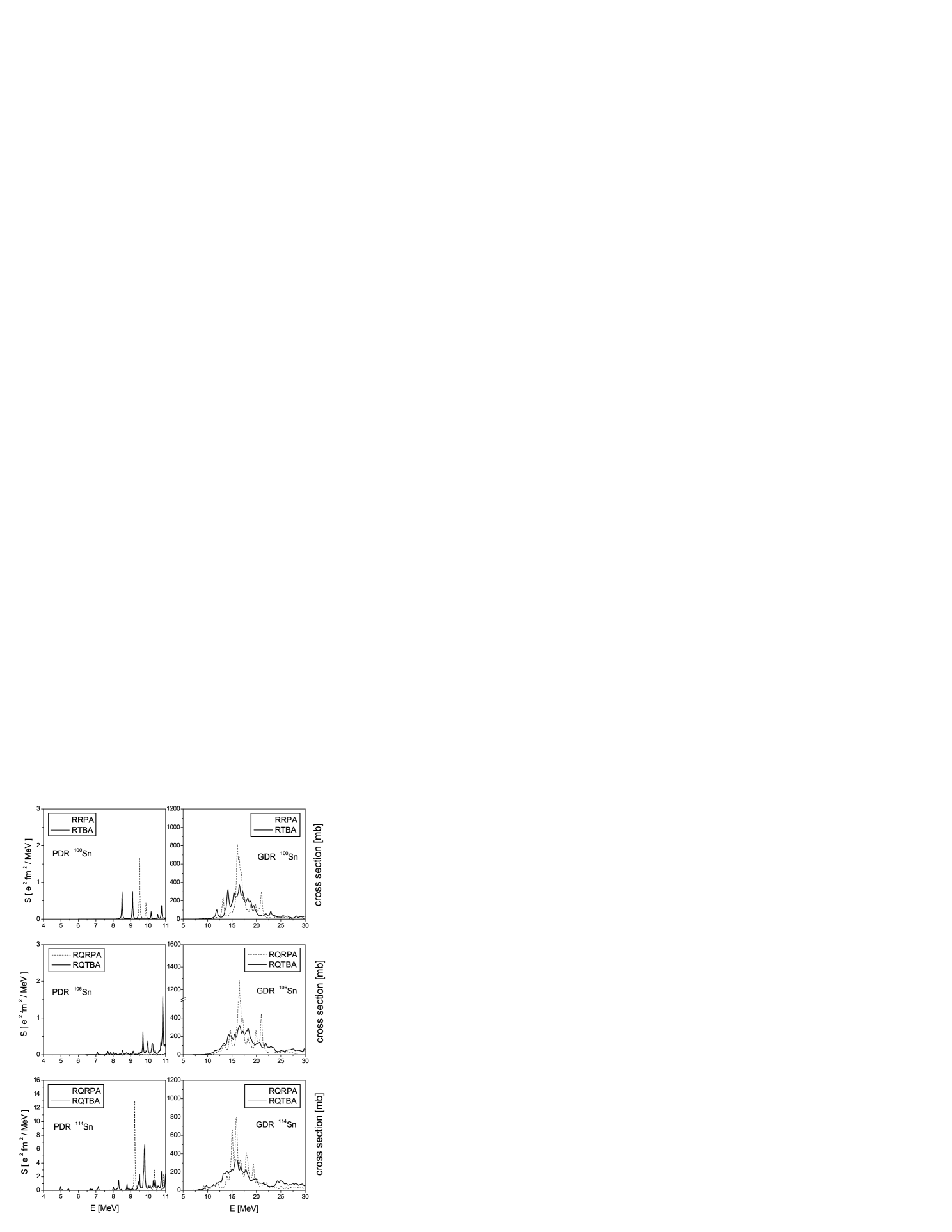
Figure 1: The calculated dipole spectra for the light tin isotopes. Right panels: photo absorption cross sections computed with the artificial width 200 keV. Left panels: the low-lying portions of the corresponding spectra in terms of the strength function, calculated with 20 keV smearing. Calculations within the RQRPA are shown by the dashed curves, and the RQTBA - by the solid curves. exfor .

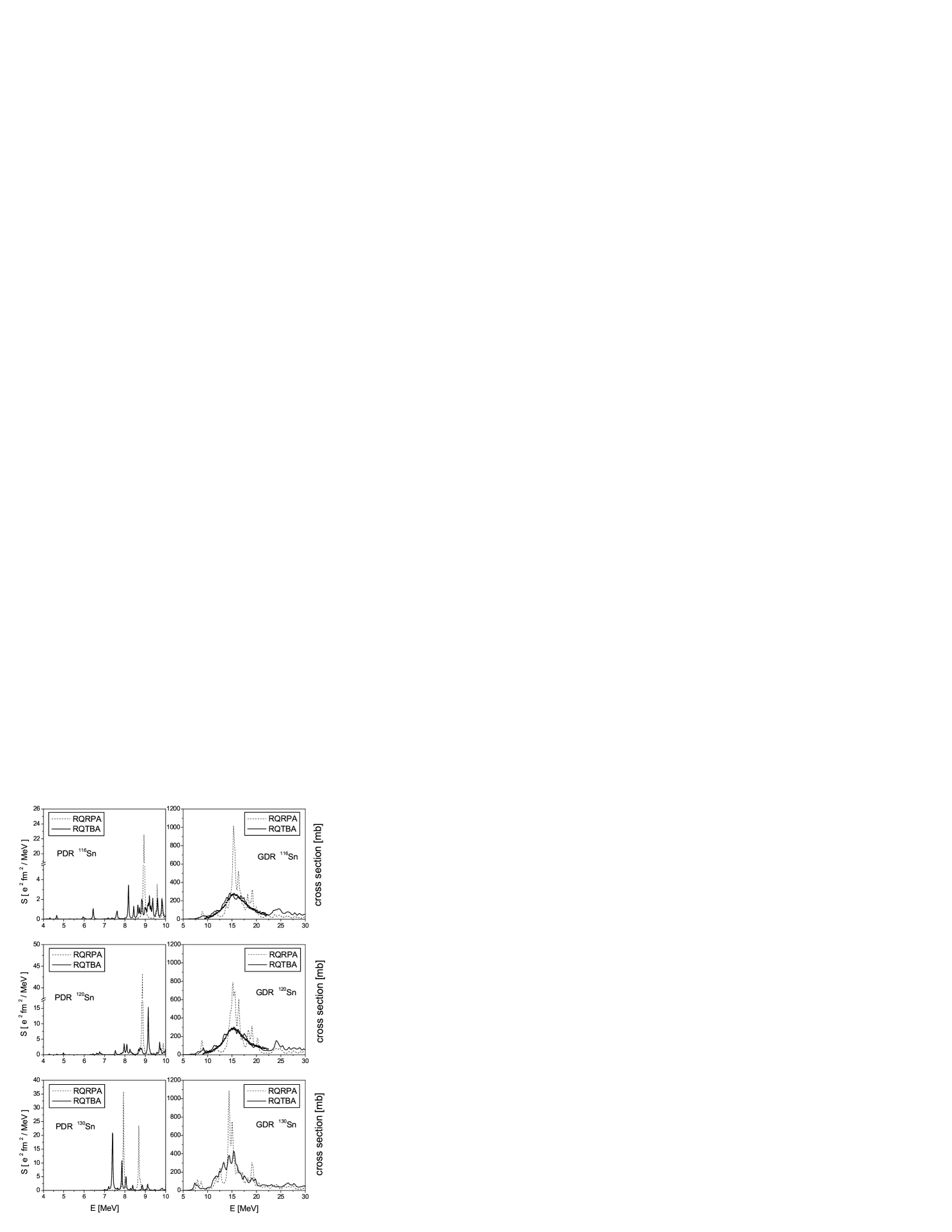
Figure 2: The same as in Fig. 1, but for heavier tin isotopes, compared to data of Ref. exfor for ^116,120Sn.

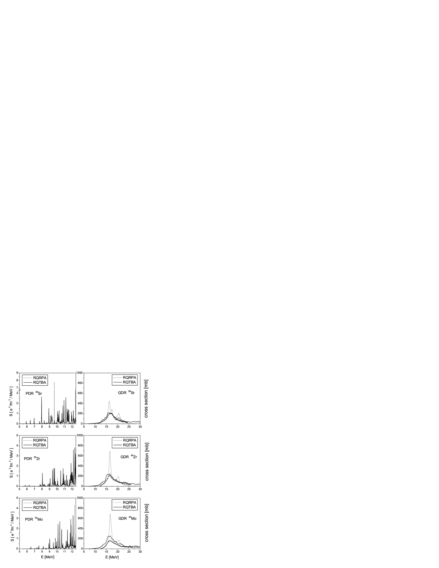
Figure 3: The same as in Fig. 1, but for $N=50$ isotopes, compared to data from Ref. exfor .

Table 1: Characteristics of the isovector dipole spectrum for the examined $N=50$ and $Z=50$ nuclei: mean energies $\langle E\rangle$, widths $\Gamma$ and EWSR values calculated with the RQRPA and with the RQRPA extended by the particle-phonon coupling (RQTBA), compared to data. The values of $\langle E\rangle$ and $\Gamma$ have been obtained by a Lorentz fit of the computed strength functions within the interval $[S_{n},3S_{n}]$ where $S_{n}$ is the neutron separation energy.

		$\langle E\rangle$	$\Gamma$	EWSR
		(MeV)	(MeV)	(%)
	RQRPA	17.36	3.46	125
88Sr	RQTBA	17.08	5.10	112
	RQRPA	17.03	3.15	124
90Zr	RQTBA	16.72	4.77	110
	Exp. ripl	16.74	4.16
	RQRPA	17.45	3.09	128
92Mo	RQTBA	17.13	4.72	113
	Exp. ripl	16.82	4.14
	RRPA	16.88	2.99	117
100Sn	RTBA	16.39	3.43	106
	RQRPA	17.17	3.07	127
106Sn	RQTBA	16.53	4.89	111
	RQRPA	16.35	3.67	126
114Sn	RQTBA	15.80	5.42	106
	RQRPA	15.95	3.11	121
116Sn	RQTBA	15.35	5.17	102
	Exp. ripl	15.56	5.08
	RQRPA	15.88	3.05	121
120Sn	RQTBA	15.31	5.33	104
	Exp. ripl	15.37	5.10
	RQRPA	15.13	3.49	115
130Sn	RQTBA	14.66	4.74	108
	Exp. Adr.05	15.9(5)	4.8(1.7)

Table 2: Integral characteristics of the isovector dipole spectrum for the examined $N=50$ and $Z=50$ nuclei: the integrated strength of the low-lying part below 10 MeV, calculated with the RQRPA and with the RQRPA extended by the particle-phonon coupling (RQTBA), compared to the available data.

		(0 - 10) MeV		(0 - 8) MeV
		$\sum B(E1)\uparrow$	$\sum EB(E1)\uparrow$	$\sum B(E1)\uparrow$	$\sum EB(E1)\uparrow$
		$(e^{2}fm^{2})$	(%)	$(e^{2}fm^{2})$	(%)
	RQRPA	0.26	0.80	0.00	0.00
88Sr	RQTBA	0.32	0.80	0.13	0.30
	Exp. KSS.04			0.141(15)	0.38(3)
	RQRPA	0.02	0.07	0.00	0.00
90Zr	RQTBA	0.34	0.90	0.07	0.15
	RQRPA	0.0049	0.01	0.00	0.00
92Mo	RQTBA	0.20	0.50	0.03	0.06
	RRPA	0.14	0.30	0.00	0.00
100Sn	RTBA	0.11	0.30	0.00	0.00
	RQRPA	0.01	0.03	0.00	0.00
106Sn	RQTBA	0.14	0.30	0.02	0.04
	RQRPA	0.84	2.00	0.00	0.00
114Sn	RQTBA	1.38	3.00	0.20	0.30
	RQRPA	1.78	4.00	0.00	0.00
116Sn	RQTBA	1.94	4.00	0.27	0.40
	Exp. Gov.98			0.204(25)
	RQRPA	3.04	6.00	0.00	0.00
120Sn	RQTBA	3.08	6.00	0.62	1.00
	RQRPA	4.04	7.00	2.09	4.00
130Sn	RQTBA	3.44	6.00	2.37	4.00
	Exp. Adr.05	3.2	7(3)

The fragmentation of the resonances, induced by the quasiparticle-phonon coupling, is a very well known result which has been obtained long ago SSV.77 ; BBBD.79 ; BB.81 (see also relatively recent calculations of electric dipole excitations in open-shell nuclei including QPC within the framework of non-relativistic approaches based on the Skyrme energy functional CB.01 ; SBC.04 as well as on the simple semi-phenomenological scheme including the single-particle continuum LT.07 ). Actually, one finds more or less a similar level of agreement between the available experimental data and the theoretical predictions of these approaches. We notice, however, that, in general, our self-consistent relativistic approach reproduces the shapes and often the mean energies of giant dipole resonances better than the other above mentioned approaches, that could be attributed to the more realistic form of the meson-exchange force and to the fully consistent calculation scheme.

From Figs. 2, 3 one can see that the envelopes of the calculated GDR in ^116,120Sn between 10 and 22 MeV and in ⁹⁰Zr, ⁸⁸Sr between 12 and 25 MeV are rather close to the experimental cross sections. The deviations from the smooth Lorentz shape observed in experiments could be attributed to some minor drawbacks of our approach and calculation scheme: neglecting of the more complicated, than the $2q\otimes phonon$, configurations by the time blocking, discretized continuum, restriction of the phonon subspace by the only low-lying modes, and, at last, too simple model for the pairing force. Nevertheless, we find that the agreement with the data for the GDR cross sections in these nuclei is very good, especially taking into account the fact, that our approach is fully consistent and contains no any fit additionally to the fit of the RMF energy functional parameters NL3 which are fixed in the very beginning and used for the entire nuclear chart. Therefore, we conclude that the main mechanisms which are responsible for the damping of the GDR are taken into account correctly and consistently.

V Outlook and conclusions

The Relativistic Quasiparticle Time Blocking Approximation (RQTBA) has been developed and applied for nuclear structure calculations. The physical content of this approach is the quasiparticle-vibration coupling model based on the relativistic energy density functional and the relativistic QRPA. The approach is formulated for a system with an even particle number in terms of the Bethe-Salpeter equation for the $ph$-channel in the doubled space to describe a response of the system in an external field and its spectral characteristics.

The static part of the single-quasiparticle self-energy is determined by the relativistic energy functional with the parameter set NL3 based on a one-meson exchange interaction with a non-linear self-coupling between the mesons. An independent phenomenologically parameterized term is introduced into the relativistic energy functional to describe pairing correlations which are considered to be a non-relativistic effect and treated in terms of Bogoliubov’s quasiparticles and, in the application, within the BCS approximation. In order to take the QPC into account in a consistent way, we have first calculated the amplitudes of this coupling within the self-consistent RQRPA with the static interaction. Then, the calculated QPC energy-dependent self-energy was introduced into the Dirac-Hartree-Bogoliubov equation for the single-quasiparticle wave function and into the equivalent Dyson equation for a single-quasiparticle Green’s function. The Bethe-Salpeter equation for the response function in the doubled space contains the energy-dependent induced interaction connected with the energy-dependent self-energy by the consistency condition. The BSE has been formulated and solved in both Dirac-Hartree-BCS and momentum-channel representations.

In order to solve the BSE in the quasiparticle time blocking approximation, the time-projection technique is used to block the two-quasiparticle propagation through the states which have more complicated structure than $2q\otimes phonon$. The nuclear response is then explicitly calculated on the $2q\otimes phonon$ level by summation of infinite series of Feynman’s diagrams. In order to avoid double counting of the QPC effects a proper subtraction of the static QPC contribution has been performed. Since the parameters of density functional for the static RHB description have been adjusted to experiment they include already essential ground state correlations.

The RQTBA introduced in the first sections of this work is applied for the calculation of spectroscopic characteristics of the isovector dipole excitations in the wide energy range up to 30 MeV for spherical open-shell nuclei, in particular for the isotopes ^{100,106,114,116,120,130}Sn (Z=50) and ⁸⁸Sr, ⁹⁰Zr, ⁹²Mo (N=50). The QPC leads to a significant spreading width of the GDR as compared to RQRPA calculations and causes the strong fragmentation of the pygmy dipole mode and its spreading to lower energies. This is in an agreement with experimental data as well as with the results obtained within the non-relativistic approaches.

The good agreement of our results with the experimental data obtained without any additional adjustable parameters for a large number of semi-magic nuclei, confirms the universality of the RMF energy functional and the predictive power of our approach. We hope, that some of the minor drawbacks in these calculations can be overcome by using in future an improved version of the density functional both in the $ph$- and in the $pp$-channel.

ACKNOWLEDGEMENTS

Helpful discussions with Prof. D. Vretenar are gratefully acknowledged. This work has been supported in part by the Bundesministerium für Bildung und Forschung under project 06 MT 246 and by the DFG cluster of excellence “Origin and Structure of the Universe” (www.universe-cluster.de). E. L. acknowledges the support from the Alexander von Humboldt-Stiftung. P.R. thanks for the support provided by the Ministerio de Educación y Ciencia, Spain, under the number SAB2005-0025. V. T. acknowledges financial support from the Deutsche Forschungsgemeinschaft under the grant No. 436 RUS 113/806/0-1 and from the Russian Foundation for Basic Research under the grant No. 05-02-04005-DFG_a.

References

- (1) P. Ring, Prog. Part. Nucl. Phys. 37, 193 (1996).
- (2) D. Vretenar, A. V. Afanasjev, G. A. Lalazissis, and P. Ring, Phys. Rep. 409, 101 (2005).
- (3) Y. K. Gambhir, P. Ring, and A. Thimet, Ann. Phys. (N.Y.) 198, 132 (1990).
- (4) G. A. Lalazissis, D. Vretenar, and P. Ring, Euro. Phys. J. A22, 37 (2004).
- (5) G. A. Lalazissis, M. M. Sharma, P. Ring, and Y. K. Gambhir, Nucl. Phys. A608, 202 (1996).
- (6) T. Bürvenich, M. Bender, J. A. Maruhn, and P.-G. Reinhard, Phys. Rev. C69, 014307 (2004).
- (7) J. Meng and P. Ring, Phys. Rev. Lett. 77, 3963 (1996).
- (8) G. A. Lalazissis, D. Vretenar, and P. Ring, Phys. Rev. C69, 017301 (2004).
- (9) G. A. Lalazissis, D. Vretenar, and P. Ring, Nucl. Phys. A650, 133 (1999).
- (10) W. Koepf and P. Ring, Nucl. Phys. A493, 61 (1989).
- (11) A. V. Afanasjev, P. Ring, and J. König, Nucl. Phys. A676, 196 (2000).
- (12) P. Ring, Z.-Y. Ma, N. Van Giai, D. Vretenar, A. Wandelt, and L.-G. Cao, Nucl. Phys. A694, 249 (2001).
- (13) N. Paar, P. Ring, T. Nikšić, and D. Vretenar, Phys. Rev. C67, 034312 (2003).
- (14) A. Ansari, Phys. Lett. B623, 37 (2005).
- (15) A. Ansari and P. Ring, Phys. Rev. C74, 054313 (2006).
- (16) N. Paar, T. Nikšić, D. Vretenar, and P. Ring, Phys. Rev. C69, 054303 (2004).
- (17) D. Vretenar, T. Nikšić, and P. Ring, Phys. Rev. C65, 024321 (2002).
- (18) E. Litvinova and P. Ring, Phys. Rev. C73, 044328 (2006).
- (19) T. Nikšić, D. Vretenar, and P. Ring, Phys. Rev. C73, 034308 (2006).
- (20) T. Nikšić, D. Vretenar, and P. Ring, Phys. Rev. C74, 054309 (2006).
- (21) E. Litvinova, P. Ring, and V. I. Tselyaev, Phys. Rev. C75, 064308 (2007).
- (22) E. Litvinova, P. Ring, and D. Vretenar, Phys. Lett. B647, 111 (2007).
- (23) V. I. Tselyaev, Yad. Fiz. 50, 1252 (1989).
- (24) V. I. Tselyaev, Sov. J. Nucl. Phys. 50, 780 (1989).
- (25) S. P. Kamerdzhiev, G. Y. Tertychny, and V. I. Tselyaev, Phys. Part. Nucl. 28, 134 (1997).
- (26) S. P. Kamerdzhiev, J. Speth, and G. Y. Tertychny, Phys. Rep. 393, 1 (2004).
- (27) V. I. Tselyaev, Phys. Rev. C75, 024306 (2007).
- (28) E. V. Litvinova and V. I. Tselyaev, Phys. Rev. C75, 054318 (2007).
- (29) V. G. Soloviev, Theory of Atomic Nuclei: Quasiparticles and Phonons (Institute of Physics, Bristol and Phyladelphia, USA, 1992), textbook on QPM.
- (30) C. A. Bertulani and V. Y. Ponomarev, Phys. Rep. 321, 139 (1999).
- (31) G. Colò and P. F. Bortignon, Nucl. Phys. A696, 427 (2001).
- (32) A. Bohr and B. Mottelson, Nuclear Structure (Benjamin, Reading, Mass., 1975), Vol. II.
- (33) J. G. Valatin, Phys. Rev. 122, 1012 (1961).
- (34) H. Kucharek, Phd thesis, Technical University of Munich (unpublished), 1989.
- (35) H. Kucharek and P. Ring, Z. Phys. A339, 23 (1991).
- (36) M. Serra, A. Rummel, and P. Ring, Phys. Rev. C65, 014304 (2002).
- (37) M. Serra and P. Ring, Phys. Rev. C65, 064324 (2002).
- (38) L. P. Gor’kov, Sov. Phys. JETP 34, 505 (1958).
- (39) W. Brenig and H. Wagner, Z. Phys. 173, 484 (1963).
- (40) J. D. Walecka, Ann. Phys. (N.Y.) 83, 491 (1974).
- (41) B. D. Serot and J. D. Walecka, Adv. Nucl. Phys. 16, 1 (1986).
- (42) J. Boguta and A. R. Bodmer, Nucl. Phys. A292, 413 (1977).
- (43) S. A. Fayans, S. V. Tolokonnikov, E. L. Trykov, and D. Zawischa, Nucl. Phys. A676, 49 (2000).
- (44) G. F. Bertsch and H. Esbensen, Ann. Phys. (N.Y.) 209, 327 (1991).
- (45) K. Capelle and E. K. U. Gross, Phys. Rev. B59, 7140 (1999).
- (46) A. A. Abrikosov, L. P. Gor’kov, and I. E. Dzyaloshincki, Methods of Quantum Field Theory in Statistical Physics (Prentice Hall, Engelwood Cliffs, New York, 1963).
- (47) V. G. Soloviev, C. Stoyanov, and A. I. Vdovin, Nucl. Phys. A288, 376 (1977).
- (48) G. F. Bertsch, P. F. Bortignon, R. A. Broglia, and C. H. Dasso, Phys. Lett. B80, 161 (1979).
- (49) P. F. Bortignon and R. A. Broglia, Nucl. Phys. A371, 405 (1981).
- (50) G. Colò, P. F. Bortignon, N. Van Giai, A. Bracco, and R. Broglia, Phys. Lett. B276, 279 (1992).
- (51) D. Sarchi, P. F. Bortignon, and G. Colo, Phys. Lett. B601, 27 (2004).
- (52) J. F. Dawson and R. J. Furnstahl, Phys. Rev. C42, 2009 (1990).
- (53) Z.-Y. Ma, N. Van Giai, H. Toki, and M. L’Huillier, Phys. Rev. C42, 2385 (1997).
- (54) D. Peña Arteaga and P. Ring, to be published (2007).
- (55) V. I. Tselyaev, E. Litvinova, D. Pena, and P. Ring, to be published (2008).
- (56) T. Gonzales-Llarena, J. L. Egido, G. A. Lalazissis, and P. Ring, Phys. Lett. B379, 13 (1996).
- (57) P. Ring and P. Schuck, The nuclear many-body problem (Springer, Heidelberg, 1980).
- (58) P. Bonche, H. Flocard, P.-H. Heenen, S. J. Krieger, and M. S. Weiss, Nucl. Phys. A443, 39 (1985).
- (59) Z.-Y. Ma, A. Wandelt, N. Van Giai, D. Vretenar, P. Ring, and L.-G. Cao, Nucl. Phys. A703, 222 (2002).
- (60) G. A. Lalazissis, J. König, and P. Ring, Phys. Rev. C55, 540 (1997).
- (61) P. Papakonstantinou, Euro. Phys. Lett. 78, 12001 (2007).
- (62) Experimental Nuclear Reaction Data, http://www-nds.iaea.or.at/exfor/exfor00.htm.
- (63) Reference Input Parameter Library, Version 2, http://www-nds.iaea.org/RIPL-2/.
- (64) P. Adrich et al., Phys. Rev. Lett. 95, 132501 (2005).
- (65) K. Govaert et al., Phys. Rev. C57, 2229 (1998).
- (66) L. Käubler, H. Schnare, and R. Schwengner et al., Phys. Rev. C70, 064307 (2004).
- (67) N. Tsoneva, H. Lenske, and C. Stoyanov, Nucl. Phys. A731, 273 (2004).
- (68) N. Tsoneva and H. Lenske, arXiv:0706.2989[nucl-th]; arXiv:0706.4204[nucl-th] (2007).