X-ray spectra from magnetar candidates. I. Monte Carlo simulations in the non-relativistic regime

Abstract

The anomalous X-ray pulsars and soft $\gamma$-repeaters are peculiar high-energy sources believed to host a magnetar, an ultra-magnetized neutron star with surface magnetic field in the PetaGauss range. Their persistent, soft X-ray emission exhibit a two component spectrum, usually modeled by the superposition of a blackbody and a power-law tail. It has been suggested that the $\sim 1$–10 keV spectrum of AXPs/SGRs forms as the thermal photons emitted by the cooling star surface traverse the magnetosphere. Magnetar magnetospheres are, in fact, likely different from those of ordinary radio-pulsars, since the external magnetic field may acquire a toroidal component as a consequence of the deformation of the star crust induced by the super-strong interior field. In a twisted magnetosphere, the supporting currents can provide a large optical depth to resonant cyclotron scattering. The thermal spectrum emitted by the star surface will be then distorted because primary photons gain energy in the repeated scatterings with the flowing charges, and this may provide a natural explanation for the observed spectra. In this paper we present 3D Monte Carlo simulations of photon propagation in a twisted magnetosphere. Our model is based on a simplified treatment of the charge carriers velocity distribution which however accounts for the particle collective motion, in addition to the thermal one. Present treatment is restricted to conservative (Thomson) scattering in the electron rest frame. The code, nonetheless, is completely general and inclusion of the relativistic QED resonant cross section, which is required in the modeling of the hard ($\sim 20$–200 keV) spectral tails observed in the magnetar candidates, is under way. The properties of emerging spectra have been assessed under different conditions, by exploring the model parameter space, including effects arising from the viewing geometry. Monte Carlo runs have been collected into a spectral archive which has been then implemented in the X-ray fitting package XSPEC. Two tabulated XSPEC spectral models, with and without viewing angles, have been produced and applied to the 0.1–10 keV XMM-Newton EPIC-pn spectrum of the AXP CXOU J1647-4552 .

1 Introduction

Over the last few years, increasing observational evidence has gathered in favour of the existence of “magnetars”, i.e. neutron stars (NSs) endowed with an ultra-strong magnetic field ($B\approx 10^{14}-10^{15}$ G), much higher than the critical threshold at which quantum electro-dynamical (QED) effects become important ($B_{crit}\sim 4.4\times 10^{13}$ G). The existence of these objects has been first proposed in the early ’90s by Duncan & Thompson (1992) and Thompson & Duncan (1993), who suggested that, soon after the core collapse following the supernova explosion, convective motions can strongly amplify the seed magnetic field via helical dynamo action. The magnetar model, initially developed to describe the phenomenology of the so-called soft $\gamma$-ray repeaters (SGRs), namely the emission of strong bursts, the fast spin period evolution and the persistent X-ray luminosity, is currently believed to successfully reproduce the properties of another class of peculiar NSs, the anomalous X-ray pulsars (AXPs). Although alternative models, invoking accretion from a fossil disc, are not completely ruled out by observations as yet (see e.g. Van Paradijs et al., 1995; Chatterejee et al., 2000; Perna et al., 2000), the recent detection of SGR-like bursts from five AXPs (Gavriil et al., 2002; Kaspi et al., 2003; Woods et al., 2005; , 2006; Krimm et al., 2006) has strengthened the connection between the two groups and pushed forward the interpretation of AXPs as magnetars.

Both classes of sources, SGRs and AXPs, are characterized by spin periods in a narrow range (5–12 s), a typical persistent X-ray luminosity of $\approx 10^{34}$–10${}^{36}\ {\rm erg\,s}^{-1}$, no evidence for Doppler shifts in the light curve, lack of bright optical companions (favouring an interpretation in terms of isolated objects), and a spin-down in the range 10^-13–10${}^{-10}\ {\rm s\,s}^{-1}$. In particular, the magnetar scenario appears promising in providing an alternative mechanism (namely the ultra-strong magnetic field) to power their high X-ray luminosity, which can not be otherwise explained in terms of more conventional processes, as accretion from a binary companion or injection of rotational energy in the pulsar wind/magnetosphere. Besides, measurements of period and period derivative, assuming that spin-down is associated to magneto-dipolar losses, are strongly suggestive of the presence of an ultra-strong magnetic field, $B>B_{crit}$.

The soft X-ray spectra of AXPs are generally well described by a two component model, consisting of a blackbody with $kT\sim$ 0.4–0.5 keV, and a power-law with photon index $2\la\Gamma\la 4$ (e.g. Woods & Thompson, 2006, and references therein). In some cases, SGRs spectra have been fit with a single power-law component, but recent deep observations showed that, also for these sources, a blackbody component is often required (Mereghetti et al., 2005b, 2006). Despite the fact that the blackbody plus power-law model has been routinely applied to magnetar candidate spectra for several years, attempts to provide a physical interpretation for these two components have just begun.

Recently it has been proposed that this phenomenological spectral model mimics a situation in which soft seed photons emerging, for instance, from the neutron star surface are boosted to higher energies by efficient resonant cyclotron scattering (RCS) from magnetospheric charged particles, leading to the formation of a power-law high-energy tail. The basic idea has been discussed by Thompson, Lyutikov & Kulkarni (2002) (TLK in the following), who suggested that a possible difference between SGRs/AXPs and standard radio-pulsars is that in the former the internal magnetic field is highly twisted, up to $\sim 10$ times the external dipole. Stresses imparted to the star crust by the strong toroidal component of the internal magnetic field cause the crust to deform. This produces, in turn, a displacement of the footpoints of the external magnetic field lines with the net result that, at intervals, the external (initially dipolar) field may acquire a toroidal component, i.e. it may twist up as well. Twisted magnetospheres are threaded by currents, substantially in excess of the Goldreich-Julian current. As shown by TLK, charge carriers may provide large optical depth to resonant cyclotron scattering so that soft (thermal) photons produced at the star surface gain energy through repeated collisions with the moving charges. Since the electron distribution is spatially extended, and the resonant cross section depends on the local value of $B$, it is expected that repeated scatterings lead to the formation of a high-energy tail, instead of a narrow cyclotron line. At least qualitatively, this scenario may also explain the correlation between spectral hardening, luminosity and increase in bursting/glitching activity that has been recently discovered in the long-term evolution of a few sources (Mereghetti et al., 2005b; Rea et al., 2005; Campana et al., 2007).

The problem of computing the X-ray spectrum emerging from twisted magnetospheres has been previously tackled using a simplified one-dimensional approach by Lyutikov & Gavriil (2006), and a systematic application to X-ray data has been presented by Rea et al. (2008) (see also Rea et al. 2007a). More recently, 3-D Monte Carlo calculations have been presented by Fernandez & Thompson (2007), although these spectra have never been applied to fit X-ray observations. Both these investigations treat resonant cyclotron scattering in the non-relativistic regime, and neglect electron recoil, i.e. use the resonant cross section in the particle frame in the (magnetic) Thomson limit.

Interestingly, thanks to INTEGRAL, it has been recently found that AXPs and SGRs exhibit very hard high-energy tails ($\Gamma\sim 1$) which can extend up to $\sim 200$ keV (Kuiper et al., 2006; den Hartog et al., 2006; Revnivtsev et al., 2004; Mereghetti et al., 2005a; Molkov et al., 2005; Götz et al., 2006). This discovery come somewhat as a surprise, being the persistent spectra of these sources below $\sim 10$ keV rather soft, and changed our view of magnetars, suggesting that their luminosity might well be dominated by the hard, rather than soft, X-ray component. The origin of such high energy tails is presently unclear, but, again, most of the scenarios proposed so far invoke emission from magnetospheric particles. Quite recently, Thompson & Belobodorov (2005) discussed how soft gamma-rays may be produced in a twisted magnetosphere, suggesting two different mechanisms: either thermal bremsstrahlung emission from the surface region heated by returning currents, or synchrotron emission from pairs created higher up ($\sim$ 100 km) in the magnetosphere. However, an alternative possibility is that the high-energy tails are again created by resonant magnetic Compton up-scattering of soft X-ray photons. In order to boost efficiently soft photons up to a few hundred keVs, scattering must occur off a non-thermal population of relativistic electrons (or pairs), possibly located close to the stellar surface (Baring & Harding, 2007). A quantitative calculation of the expected spectra, which necessarily requires a correct description of relativistic effects, has not been put forward as yet.

In this paper, the first in a series devoted to investigate the X-/soft $\gamma$-ray persistent spectrum of magnetar candidates, we lay out the physical bases of our model and present a Monte Carlo code which is used to follow the spectral modifications as the soft seed photons get progressively up-scattered in the magnetosphere of an ultra-magnetized neutron star. Our present goal is to test, by direct comparison with observations, if RCS spectra are capable of accounting for the observed properties of the soft X-ray emission ($\la 10$ keV) of SGRs/AXPs. To this end, we adopt a non-relativistic (Thomson) description for the scattering process. However, the numerical scheme is completely general and is explicitly designed to incorporate the fully QED cross sections and to deal with more complex magnetic configurations. The former, together with an application to the hard X-ray tails detected by INTEGRAL, will be the scope of forthcoming papers (Nobili, Turolla & Zane in preparation). In many respects the present investigation follows an approach similar to that of Fernandez & Thompson (2007), and we will refer to this paper for some useful expressions. The two treatments, however, differ in a number of ways. In particular, the present model includes the angular and frequency dependence of seed photons in a more general way and a different prescription for the current velocity distributions. Differences and similarities between the two methods will be discussed along the paper, when relevant.

The paper is organized as follows. In §2 we lay out and scrutinize the physical bases of our model. The Monte Carlo method and its coding is described in §3, while in §4 we present the computed spectra and discuss their properties. The implementation in XSPEC of our model is described in §5 where also a preliminary fit is reported. Discussion follows in §6.

2 The model

In this section we discuss in some detail the main ingredients used in our computation of the soft ($\sim 0.1$–10 keV) X-ray spectrum emitted by magnetar candidates.

2.1 External magnetic field geometry

The first ingredient of our computation is a prescription for the magnetic field geometry. Monte Carlo techniques are suitable for handling complicated 3D configurations, and our code is completely general from this point of view. However, for the sake of simplicity, in this paper we restrict ourselves to the axially symmetric twisted magnetosphere configurations studied by TLK, in which case the (numerical) solution of the magnetostatic, force-free equilibrium is straightforward. Accordingly, we report here only those expressions that are needed to facilitate the reading of this paper, and refer to TLK for all details.

The starting point is the force-free equation $\vec{j}\times\vec{B}=0$ where $\vec{j}$ and $\vec{B}$ are the current and the external field respectively. Under the assumption of axial symmetry, this equation can be written as $\nabla\times\vec{B}=\alpha({\cal P})\vec{B}$ with ${\cal P}={\cal P}(r,\theta)$ the flux parameter. A major simplification arises by restricting to self-similar configurations, ${\cal P}={\cal P}_{0}r^{-p}F(\cos\theta)$, in which case the problem reduces to the solution of a second order eigenvalue differential equation for $F(\cos\theta)$, that can be solved numerically for each value of the parameter $0\leq p\leq 1$. The latter univocally fixes the magnetic configuration, a part for a scale factor $B_{pole}$ (see below). The boundary conditions are chosen in such a way that the resulting axially-symmetric configuration corresponds to a core-centered, twisted, dipolar field (see §6 for a discussion). The polar components of the magnetic field are then (see again TLK for all details)

$$B_{r} = -\frac{B_{pole}}{2}\left(\frac{R_{NS}}{r}\right)^{2+p}\frac{dF}{d\cos\theta}$$ (1)

$$B_{\theta} = \frac{B_{pole}}{2}\left(\frac{R_{NS}}{r}\right)^{2+p}\frac{pF}{\sin\theta}$$

$$B_{\phi} = B_{\theta}\left[\frac{C}{p\left(1+p\right)}\right]^{1/2}F^{1/p}\,,$$

where the constant $C$ is an eigenvalue which depends on $p$ only, $R_{NS}$ is the neutron star radius and $B_{pole}$ is the value of the magnetic field at the pole. The net twist angle is defined as

$$\Delta\phi_{N-S}=\lim_{\theta_{0}\to 0}2\int_{\theta_{0}}^{\pi/2}\frac{B_{\phi}}{B_{\theta}}\frac{d\theta}{\sin\theta}$$ (2)

and is a function of the parameter $p$. As a consequence, either $p$ or $\Delta\phi_{N-S}$ can be used to label each model in the sequence.

2.2 Magnetospheric currents

Once the magnetic structure is known, in the force-free approximation the spatial density of the magnetospheric particles is automatically fixed by

$$n_{e}(\vec{r},\beta)=\frac{p+1}{4\pi e}\left(\frac{B_{\phi}}{B_{\theta}}\right)\frac{B}{r|\langle\beta\rangle|}\,,$$ (3)

where $\langle\beta\rangle$ is the average charge velocity (in units of $c$; see below). The above expression gives the co-rotation charge density of the space charge-limited flow of ions and electrons from the NS surface, that, due to the presence of closed loops in a twisted field, is much larger than the Goldreich-Julian density, $n_{GJ}$. Moreover, it is important to note that, while a space charge-limited flow with $n=n_{GJ}$ requires currents flowing in opposite directions from the two poles, for the case at hand there is a well defined flow direction which is the same from north to south. This breaks the symmetry between the two star hemispheres, and implies that the observed spectrum will be different when viewed from the north or the south pole. Clearly, because of charge neutrality, the electron current must be balanced by ions flowing in the opposite direction. However, ions are heavier, they are not lifted much in the magnetosphere and tend to move closer to the star surface. Photons may scatter off ions, but this is likely to give rise at most to a narrow absorption feature at the ion cyclotron energy (see TLK and Fernandez & Thompson 2007). For this reason, the ion current is not considered here, together with pair creation, that can further complicate the relation between charge and current density by introducing bidirectional flows (see §6 for a discussion). In a genuinely static twist ($\partial\vec{B}/\partial t=0$) the electric and magnetic fields are orthogonal. This implies that the voltage drop between the footpoints of a field line vanishes since $E_{\parallel}=0$, so that there is no force that can extract particles from the surface and lift them against gravity thus initiating the current $\vec{j}_{B}=c\nabla\times\vec{B}/4\pi$ requested to support the twist. However, as discussed in Beloborodov & Thompson (2007), once implanted, the twist has necessary to decay precisely to provide the potential drop required to accelerate charges. A non-vanishing $E_{\parallel}$ is maintained by self-induction and the twist evolution is regulated by the balance between the conduction current $j$ and $j_{B}$, $\partial E_{\parallel}/\partial t=4\pi(j_{B}-j)$. If $j<j_{B}$ the magnetosphere becomes charge starved and $E_{\parallel}$ grows at the expenses of the magnetic field, injecting more charges into the magnetosphere. On the other hand, when $j>j_{B}$ the field decreases reducing the current. The magnetosphere is then in dynamical (quasi)equilibrium with $j\sim j_{B}$ over a timescale $<t_{decay}$, where $t_{decay}\approx$ a few years is the twist decay time (Beloborodov & Thompson, 2007).

The second key ingredient is the velocity distribution of the magnetospheric charges. This is a crucial and still largely unexplored issue (see however Beloborodov & Thompson, 2007, and §6). Nevertheless, in a strong magnetic field the electron distribution is expected to be largely anisotropic: $e^{-}$ stream freely along the field lines, while they are confined in a set of cylindrical Landau levels in the plane perpendicular to $\vec{B}$. In order to mimic such scenario, we assume a 1-D Maxwellian distribution at a given temperature $T_{e}$, superimposed to a bulk motion with velocity $v_{bulk}$, as measured in the stellar frame. The (invariant) distribution function turns out to be

$${\frac{dn_{e}}{d(\gamma\beta)}}=\displaystyle{\frac{n_{e}\,\exp{(-\gamma^{\prime}/\Theta_{e})}}{2\,K_{1}(1/\Theta_{e})}}=n_{e}f_{e}(\vec{r},\gamma\beta)$$ (4)

where $\gamma^{\prime}=\gamma\gamma_{bulk}(1-\beta\beta_{bulk})$, $\Theta_{e}=kT_{e}/m_{e}c^{2}$, $K_{1}$ is the modified Bessel Function of the first order and $f_{e}=\gamma^{-3}n_{e}^{-1}dn_{e}/d\beta$ is the momentum distribution function. We consider $T_{e}$ and $\beta_{bulk}=v_{bulk}/c$ as free parameters in our model, and, although this is definitely a simplification, we assume that both do not depend on position. This expression differs from that used by Fernandez & Thompson (2007) (their equation [19]) inasmuch they do not include the effects of collective (bulk) velocity (which is necessary to reproduce the current flow), but only those of the $e^{-}$ local velocity distribution (either thermal, as in the present case, or non-thermal). In other words, we assume that electrons move isothermically along the field lines but, at the same time, they receive the same boost from the electric field. Even in the lack of any detailed information about the charge accelerating mechanisms, we consider our choice more realistic.

2.3 Scattering cross sections

Scattering off free electrons in the presence of a strong magnetic field has been extensively treated in the literature. The non-relativistic ($B\ll B_{crit}$) expressions for the scattering cross sections in the Thomson limit (i.e. neglecting electron recoil) were derived by Ventura (1979) (see also Mészaros 1992). The complete QED compton cross sections have been presented by Herold (1979), Daugherty & Harding (1986), and Harding & Daugherty (1991). The scattering cross section depends on the incident photon polarization state and, in general, it must be computed by summing over the (infinite) virtual intermediate Landau states. Moreover, proper account has to be made for the electron spin transition and for the possibility that scattering leaves the electron in an arbitrary excited state (Raman scattering). This leads to quite cumbersome expressions (see e.g Harding & Daugherty 1991), even if one restricts to the resonant part of the completely differential cross section. On the other hand, under the typical conditions expected in a twisted magnetosphere, soft photons ($\hbar\omega\sim 1$ keV) will undergo resonant scattering when $\omega\sim\omega_{B}$ and this happens only where the field has decayed to a value $B\sim 10^{11}\,{\rm G}\ll B_{crit}$. Electron recoil starts to be important when the photon energy in the electron rest frame becomes comparable to the electron rest energy. If $\gamma$ is the mean electron Lorentz factor, this occurs at typical energies $\sim m_{e}c^{2}/\gamma$. Assuming mildly relativistic particles, the previous limit implies that conservative scattering should provide good accuracy up to photon energies of some tens of keV. This, together with the fact that resonant scattering occurs in regions where $B\ll B_{crit}$, makes the use of the (much simpler) non-relativistic (Thomson) cross section adequate. We anticipate here that, albeit supported by physical considerations, this provides only a zeroth level description and a more thorough treatment demands for the full QED cross section, as it is discussed in more detail later on (see §6). A further simplification arises because, under the typical conditions encountered in the magnetosphere, vacuum polarization dominates over plasma effects. In this situation, the two (ordinary and extraordinary) normal modes are linearly polarized.

Since radiative de-excitation occurs on a very short timescale, one can safely assume that the electron is initially in the ground state. For a particle initially at rest, the non-relativistic scattering cross sections at resonance are easily derived from the general expression given e.g. by Herold (1979) by performing the substitution

$$\frac{1}{(\omega-\omega_{B})^{2}}\to\frac{1}{(\omega-\omega_{B})^{2}+\Gamma^{2}/4}$$ (5)

where $\Gamma=(4e^{2}\omega_{B}^{2})/(3m_{e}c^{3})$ accounts for the finite transition lifetime of the excited state (e.g. Daugherty & Ventura, 1978; Ventura, 1979). Since in the present case it is $\hbar\omega_{B}\simeq\hbar\omega\sim 1$ keV, the resonance peak is so narrow and prominent that non-resonant contributions to the cross section are negligible. One can therefore take the limit

$$\lim_{\Gamma\to 0}\frac{\Gamma}{(\omega-\omega_{B})^{2}+\Gamma^{2}/4}=2\pi\delta(\omega-\omega_{B})$$ (6)

which results in

$$\displaystyle\frac{d\sigma}{d\Omega^{\prime}}\Big{|}_{1-1} =\frac{3\pi r_{0}c}{8}\delta(\omega-\omega_{B})\cos^{2}\theta\cos^{2}\theta^{\prime}$$

$$\displaystyle\frac{d\sigma}{d\Omega^{\prime}}\Big{|}_{1-2} =\frac{3\pi r_{0}c}{8}\delta(\omega-\omega_{B})\cos^{2}\theta$$

$$\displaystyle\frac{d\sigma}{d\Omega^{\prime}}\Big{|}_{2-2} =\frac{3\pi r_{0}c}{8}\delta(\omega-\omega_{B})$$

$$\displaystyle\frac{d\sigma}{d\Omega^{\prime}}\Big{|}_{2-1} =\frac{3\pi r_{0}c}{8}\delta(\omega-\omega_{B})\cos^{2}\theta^{\prime}$$

where $\theta$ ($\theta^{\prime}$) is the photon angle before (after) the scattering and $r_{0}$ is the classical electron radius. Here and in the following the index 1 (2) stands for the ordinary (extraordinary) mode.

Upon normalization, the previous expressions give the probability that an incident photon with polarization state $i$ and direction $\theta$ is scattered at angle $\theta^{\prime}$ with polarization state $j$. The total cross sections for separated processes are easily computed by integrating the previous expressions over all outgoing photon angles

$$\displaystyle\sigma_{1-1} =\int_{4\pi}d\Omega^{\prime}\frac{d\sigma}{d\Omega^{\prime}}\Big{|}_{1-1}=\frac{\pi r_{0}c}{2}\delta(\omega-\omega_{B})\cos^{2}\theta$$

$$\displaystyle\sigma_{1-2} =\int_{4\pi}d\Omega^{\prime}\frac{d\sigma}{d\Omega^{\prime}}\Big{|}_{1-2}=\frac{3\pi r_{0}c}{2}\delta(\omega-\omega_{B})\cos^{2}\theta$$

$$\displaystyle\sigma_{2-2} =\int_{4\pi}d\Omega^{\prime}\frac{d\sigma}{d\Omega^{\prime}}\Big{|}_{2-2}=\frac{3\pi r_{0}c}{2}\delta(\omega-\omega_{B})$$

$$\displaystyle\sigma_{2-1} =\int_{4\pi}d\Omega^{\prime}\frac{d\sigma}{d\Omega^{\prime}}\Big{|}_{2-1}=\frac{\pi r_{0}c}{2}\delta(\omega-\omega_{B})\,.$$

The total cross section for scattering of an incident ordinary (extraordinary) photon is obtained by summing the first (second) pair of expressions in equation (2.3). Finally, in order to determine the photon direction after scattering (i.e. the two angles $\theta^{\prime}$, $\phi^{\prime}$) in the Monte Carlo code, the following integrals are required

$$\displaystyle\frac{1}{\sigma_{i-j}}\int_{0}^{\phi^{\prime}}\int_{0}^{\pi}d\Omega^{\prime}\frac{d\sigma}{d\Omega^{\prime}}\Big{|}_{i-j} =\frac{1}{2}\phi^{\prime}$$

$$\displaystyle\frac{1}{\sigma_{1-1}}\int_{0}^{2\pi}\int_{0}^{\theta^{\prime}}d\Omega^{\prime}\frac{d\sigma}{d\Omega^{\prime}}\Big{|}_{1-1} =\displaystyle\frac{1}{\sigma_{2-1}}\int_{0}^{2\pi}\int_{0}^{\theta^{\prime}}d\Omega^{\prime}\frac{d\sigma}{d\Omega^{\prime}}\Big{|}_{2-1}=\frac{1}{2}(1-\cos^{3}\theta^{\prime})$$

$$\displaystyle\frac{1}{\sigma_{1-2}}\int_{0}^{2\pi}\int_{0}^{\theta^{\prime}}d\Omega^{\prime}\frac{d\sigma}{d\Omega^{\prime}}\Big{|}_{1-2} =\displaystyle\frac{1}{\sigma_{2-2}}\int_{0}^{2\pi}\int_{0}^{\theta^{\prime}}d\Omega^{\prime}\frac{d\sigma}{d\Omega^{\prime}}\Big{|}_{2-2}=\frac{1}{2}(1-\cos\theta^{\prime})$$

2.4 Photon propagation in the magnetosphere

The scattering cross sections discussed in §2.3 hold in the electron rest frame (ERF). In particular, both the photon ($\omega$) and the cyclotron ($\omega_{B}$) frequency entering expressions (2.3)–(2.3) are evaluated in the ERF. In the case of a charge moving with velocity $v=\beta c$ and Lorentz factor $\gamma$ with respect to a frame attached to the star, the total cross sections (eq. [2.3]) take the form

$$\displaystyle\sigma_{1-1} =\frac{1}{3}\sigma_{1-2}=\frac{\pi^{2}r_{0}c}{2}\delta(\omega-\omega_{D})\cos^{2}\theta$$

$$\displaystyle\sigma_{2-2} =3\sigma_{2-1}=\frac{3\pi^{2}r_{0}c}{2}\delta(\omega-\omega_{D})$$

where

$$\omega_{D}=\frac{\omega_{B}}{\gamma(1-\beta\mu)}\,,$$ (11)

$\theta$ is the angle between the incident photon direction and the particle velocity as measured in the ERF and $\mu$ is the cosine of the same angle but measured in the stellar frame. The latter two quantities are related by the usual transformation

$$\cos\theta=\frac{\mu-\beta}{1-\beta\mu}\,.$$ (12)

Since particles are moving along $\vec{B}$, the magnetic field is unaffected by the Lorentz transformation, and the value of $B$ as measured in the stellar frame can be used to compute the cyclotron frequency $\omega_{B}$ in the ERF. It is worth stressing that $\omega$ in eqs. (2.4) is now the photon frequency in the stellar frame.

The scattering optical depth for a photon which travels a distance $d\ell$ in the magnetosphere is

$$d\tau_{ij}=d\ell\int_{\beta_{min}}^{\beta_{max}}d\beta n_{e}(\vec{r})\gamma^{3}(1-\beta\mu)\sigma_{ij}(\omega,\vec{r},\beta)f_{e}(\vec{r},\gamma\beta)$$ (13)

where the factor $1-\beta\mu$ appears because of the change of reference between the ERF and the stellar frame, $n_{e}$ is the (velocity integrated) particle density and $f_{e}$ is the (normalized) momentum distribution as defined in equations (3) and (4).

The indices $i$ and $j$ refer to the initial and final photon polarization states and $[\beta_{min},\,\beta_{max}]$ is the charge velocity spread. As pointed out by Fernandez & Thompson (2007), the integral in equation (13) can be readily calculated by exploiting the $\delta$-function in the scattering cross section. Denoting by

$$\beta_{1,2}=\frac{1}{\mu^{2}+(\omega_{B}/\omega)^{2}}\left[\mu\pm\frac{\omega_{B}}{\omega}\sqrt{(\omega_{B}/\omega)^{2}+\mu^{2}-1}\right]$$ (14)

the two roots of the quadratic equation $\omega=\omega_{D}$, the $\delta$-function in frequency can be transformed into a $\delta$-function in velocity

$$\delta(\omega-\omega_{D})= \frac{1}{\omega_{B}}\sum_{k=1,2}\frac{(1-\mu\beta_{k})^{2}}{\gamma_{k}|\mu-\beta_{k}|}\delta(\beta-\beta_{k})=\frac{\omega_{B}}{\omega^{2}}\sum_{k=1,2}\frac{1}{\gamma_{k}^{3}|\mu-\beta_{k}|}\delta(\beta-\beta_{k})\,.$$ (15)

Accordingly, the total scattering depth can be expressed as

$$d\tau_{1}= d\tau_{1-1}+d\tau_{1-2}=2\pi^{2}r_{0}c\frac{n_{e}\omega_{B}}{\omega^{2}}d\ell\sum_{k=1,2}\frac{|\mu-\beta_{k}|}{(1-\mu\beta_{k})}f_{e}(\vec{r},\gamma_{k}\beta_{k})$$ (16)

and

$$d\tau_{2}= d\tau_{2-2}+d\tau_{2-1}=2\pi^{2}r_{0}c\frac{n_{e}\omega_{B}}{\omega^{2}}d\ell\sum_{k=1,2}\frac{(1-\mu\beta_{k})}{|\mu-\beta_{k}|}f_{e}(\vec{r},\gamma_{k}\beta_{k})$$ (17)

for photons initially in the polarization state 1 and 2, respectively. These expressions are analogous to those derived by Fernandez & Thompson (2007), although their equation (33) seems to contain an error. The spatial distribution of charged particles $n_{e}$ depends, in fact, on their average velocity, i.e. the speed at which charge carriers flow, and not on the velocity of the single particle. For this reason $n_{e}$ is not evaluated at $\beta=\beta_{k}$, but at $\langle\beta\rangle$ which is, in general, a function of position (see also §2.2). Moreover, their equation (13) contains an unexpected factor $\omega_{D}$ in place of $\omega_{B}$. The reason for this is obscure since the ratio $\omega_{B}/B$ turns out to be independent of both the magnetic field and photon energy.

Once the initial photon polarization, energy and direction have been fixed, equation (16), or (17), is integrated along the photon path until a scattering occurs (see §3.2). Although general relativistic effects are certainly important, here we restrict ourselves to newtonian gravity and assume that photons move along straight lines between two successive scatterings. Proper inclusion of null geodesics in a Schwarzschild space-time, albeit conceptually simple, turned out to be computationally quite costly and we decided to dismiss it. As it is apparent from equation (15), resonant scattering may occur only when the roots $\beta_{k}$ are real, i.e. only if $(\omega_{B}/\omega)^{2}+\mu^{2}-1\geq 0$. Since $\omega_{B}$ depends (through $B$) on position alone, at every point in the magnetosphere the previous condition discriminates those pairs of photon energy and angle for which scattering is possible (Fernandez & Thompson, 2007). In case the particle velocity is always of a given sign (charge carriers all positive or negative), only the roots $\beta_{k}$ with the same sign are meaningful. If there exist two roots with the right sign (i.e. both are positive or negative), the criterion for selecting onto which particle (the one with velocity $\beta_{1}$ or $\beta_{2}$) the photon actually scatters is discussed in §3.2.

2.5 Seed photon distribution

Primary photons are assumed to be emitted by the cooling surface of the neutron star. Although, up to now, no detailed model for surface emission from a magnetar has been presented, it seems unlikely that the spatial and energy distribution of the surface-emitted photons are the same as in ordinary cooling neutron stars. In particular, being the surface heated by returning currents (e.g. TLK), the surface temperature is expected to be inhomogeneous (with the equatorial belt hotter than the polar regions) and it is unclear if a standard (i.e. in hydrostatic and radiative equilibrium) atmosphere can be present on the top of a magnetar (see however Güver, Özel & Lyutikov, 2006; Güver, Özel & Göḡüş, 2007).

On the wake of this, in order to keep our treatment as general as possible, we do not prescribe an a priori surface temperature distribution (see §3.1). In the present version of the code, the initial energy distribution is taken to be planckian for either ordinary and extraordinary photons, although other spectral distributions can be easily accommodated. Different degrees of polarization of the primary spectrum can be then obtained adding together, in different proportions, ordinary and extraordinary blackbody photons. Since the non-isotropic opacity of the stellar crust might convey radiation in a preferred direction, we introduce a beaming parameter $b\geq 1$ such that the specific intensity at the star surface takes the form

$$n_{\nu}(\mu)\propto\mu^{b-1}\frac{\nu^{2}}{\exp({h\nu/kT})-1}$$ (18)

where $\mu$ is the cosine of the angle between the initial photon direction and the magnetic field. For $b=1$ the radiation is emitted isotropically in the outward hemisphere.

3 The Monte Carlo method

The code is structured into four main blocks, as outlined below. In the first thermal photons are emitted from the stellar surface, in the second the program evaluates the optical depth of the photon as it propagates through the magnetosphere, while the third is finalized to solve the kinematics of the electron-photon scattering. Finally, escaping photons are stored. Each block is briefly described in the following.

3.1 Photon emission

Because of the intrinsic asymmetry of the model, the observed spectrum depends on both the shape, and the (longitudinal) position of the emitting region on the star surface, and the viewing direction. Moreover, as mentioned above, the star surface temperature distribution may not be isotropic. To account for these effects, the star surface is divided into $N_{\Theta}\times N_{\Phi}$ zones by means of an equally spaced $\cos\Theta$ and $\Phi$ mesh, where $\Theta$ and $\Phi$ are the magnetic colatitude and longitude. This choice guarantees that all patches have the same area, so that the number of emitted photons depends only on the patch temperature (i.e. patches at the same temperature emit the same number of photons). A different temperature may be attached to each surface patch in such a way to reproduce (up to the accuracy allowed by the finite mesh resolution) any kind of thermal surface map.

Initially we fix the coordinates of an emitting patch and assign a value for the polarization state $s$ of each seed photon, i.e. $s=1$ for the ordinary mode or $s=2$ for the extraordinary mode. All photons are emitted at the patch centre $P$. Then, a photon is extracted at random from the distribution (18). We assume that the initial photon angles are such that the azimuth (as referred to $\vec{B}$ in $P$) is uniformly distributed while $\mu=\cos\theta_{P}$ is obtained solving the equation $\mu=(U_{P})^{b}$, where $U_{P}$ is an uniform deviate and $b$ is the beaming parameter introduced in eq. (18). The coordinates of the emission point and the initial momentum univocally determine the ray along which the photon moves.

Actually, after experiencing scattering(s), some photons will reach the star surface again. Their number is fairly limited, since scattering typically occurs at a distance $R_{sc}$ of a few stellar radii. The star disc, as seen from the last scattering point, subtends a solid angle $\sim(R_{NS}/R_{sc})^{2}\la 0.1$, and this is also an upper limit to the fraction of photons which are scattered back onto the star surface. Numerical simulations show that the actual value is quite smaller, $\la 1\%$. We assume that all photons impinging on the surface are absorbed (regardless of their polarization state).

3.2 Scattering depth

In a Monte Carlo scheme the distance $\ell$ a photon of polarization state $s$ travels between two successive interactions (i.e. emission-scattering or scattering-scattering) is estimated by integrating the scattering depth $d\tau_{s}$ given by equations (16) and (17) until

$$\tau_{s}=\int_{0}^{\ell}d\tau_{s}=-\ln U$$ (19)

where $U$ is an uniform deviate. Direct numerical evaluation of the integral (19) proved, however, quite time consuming, and we found more efficient and faster to perform a stepwise integration the differential equations (16) and (17) using a fourth order Runge-Kutta method. Integration is terminated as soon as the value of the optical depth exceeds $-\ln U$ and a linear interpolation between the last two steps is used to determine with better accuracy the value of $\ell$ where $\tau_{s}=-\ln U$.

At each integration step we check if the photon still lies in the region of the $(\omega_{b}/\omega,\,\mu)$ plane where resonant scattering is allowed, i.e. if $\omega_{B}^{2}/\omega^{2}+\mu^{2}-1\geq 0$ (see §2.4). When the previous inequality is found to hold no more, we further check if the photon trajectory is bound to bring it back into the scattering permitted region or not. This is achieved by computing numerically the tangent to the photon path [in the $(\omega_{B}/\omega,\,\mu)$ plane] where $\omega_{B}^{2}/\omega^{2}+\mu^{2}-1\sim 0$ and checking if it lies in between the two limiting values $(\mu\pm 1)/(\omega_{B}/\omega)$. If not, the photon is taken to freely escape to infinity [see also figure 1 of Fernandez & Thompson (2007)]. The values of the energy and direction of the photon are then stored, the program returns to step 1, and a new seed photon is emitted.

3.3 The scattering process

Assuming that equality $\tau_{s}=-\ln U$ is verified at some distance $\ell$ from the point of the previous photon interaction, the kinematics of the scattering must be solved in order to obtain the new direction and energy of the photon. This requires the knowledge of the velocity $\beta_{k}$ of the resonant electron and the new photon polarization state. This is obtained by generating two new random numbers, $U_{1}$ and $U_{2}$, and comparing them with the ratios of the corresponding cross sections. For a photon initially in the ordinary polarization state ($s=1$), mode switching upon scattering occurs if $U_{1}>\sigma_{1-1}/(\sigma_{1-1}+\sigma_{1-2})=1/4$, while for an initially extraordinary photon ($s=2$) this happens if $U_{1}>\sigma_{2-2}/(\sigma_{2-2}+\sigma_{2-1})=3/4$. Similarly, the decision about onto which of the two resonant electrons (assuming that both values of $\beta_{k}$ are acceptable) scattering actually occurs is reached by comparing $U_{2}$ with the ratio $S_{s}(\beta_{1})/[S_{s}(\beta_{1})+S_{s}(\beta_{2})]$, where $S_{s}(\beta_{k})$ stands for each addendum in the sum at left hand side of equation (16) ([17]). If $U_{2}<S_{s}(\beta_{1})/[S_{s}(\beta_{1})+S_{s}(\beta_{2})]$, the scattering electron velocity is $\beta_{1}$, otherwise it is $\beta_{2}$. At this stage, all parameters entering the differential cross section of the process are known.

Upon scattering with a moving charge, the momentum and energy of the photon are modified. Since the cross section (2.3) are defined in the ERF, the evaluation of the scattering angles $\theta^{\prime}$ and $\phi^{\prime}$ requires a Lorentz transformation from the stellar frame to the frame comoving with the resonant electron $\beta_{k}$. For linearly polarized incoming light the distribution of the azimuthal angle is isotropic, so that $\phi^{\prime}=2\pi U_{3}$, where $U_{3}$ is an uniform deviate. Concerning the scattering angle, we note that in the non relativistic case all quantities (2.3) are proportional either to $1-\cos\theta^{\prime}$ or to $1-\cos^{3}\theta^{\prime}$. Then, after drawing a new uniform deviate $U_{4}$, the scattering angle is given by $\cos\theta^{\prime}=2U_{4}-1$ or $\cos^{3}\theta^{\prime}=2U_{4}-1$, depending on the case.

The corresponding angles in the stellar frame and, hence the new photon direction, are obtained by means of Lorentz transformations. In this frame the photon frequency is given by

$$\omega^{\prime}=\gamma_{k}^{2}\omega\,(1-\beta_{k}\mu)(1+\beta_{k}\cos\theta^{\prime})\,.$$ (20)

Finally, once energy and momentum of the scattered photon are known the computation proceeds starting again from point 3.2, integrating equations (16) or (17) along the new photon path.

3.4 Photons storage

Escaping photons are collected on the “sky at infinity”, i.e. on a spherical surface located sufficiently farther out to see the star (and its magnetosphere) as point-like. We introduce an angular grid $(\Theta_{s},\,\Phi_{s})$ which divides the “sky at infinity” in a fixed number of patches, similarly to what has been done for the stellar surface. When the escape condition (see §2.4) is met, the two angles $\Theta$ and $\Phi$ which characterize the ray relative to the star centre are computed from the photon momentum and the sky patch hit determined. Counts are stored in a three-dimensional array, the first two indices of which label the sky patch while the third the photon energy. This allows to analyze the resulting spectra in different directions of observation when a large number of events are processed. Each run involves $N_{tot}$ photons, and is performed changing the initial polarization states $s$ and the co-ordinates of the emitting patch. The resulting spectrum is obtained by superposition of the various emitting patches.

4 Results

Our Monte Carlo code, written in FORTRAN90, proved to be efficient and relatively fast. Despite the complexity of the whole procedure, we can process about 7000 photons/s on a dual-core Xeon 2.8 GHz machine. The CPU time for a typical production run (several million photons) is 10–20 min. We stress that the result of each run is a 3D array which gives the number of counts at different positions on the sky and at different energies (see §3.4). Further manipulations (e.g. to account for viewing angles, or to derive the pulse shape, see below) are performed at the post-processing level by means of IDL scripts, at negligible computational cost. In the following subsections we discuss the general properties of our spectral models.

4.1 Spectra

In order to explore the role of the different parameters we computed a set of spectra, by evolving $N_{patch}=150,000$ photons for $N_{\Theta}\times N_{\Phi}=8\times 4=32$ surface patches (i.e. each model has $N_{tot}=4,800,000$ photons). We assume that the star surface is at constant temperature, and that the seed radiation is isotropic ($b=1$, see § 2.5) and completely polarized, either in the ordinary or extraordinary mode. Furthermore, we treat the case of an aligned rotator, i.e. the spin and magnetic axes coincide. Photons are collected onto a $N_{\Theta_{s}}\times N_{\Phi_{s}}=10\times 10$ angular grid on the sky, and in $N_{E}=50$ energy bins in the range 0.1–100 keV. The magnetic field has been fixed at $B=10^{14}$ G and the surface temperature at $kT=0.5$ keV. The mean and the maximum number of scatterings per photon are in the ranges $\sim 0.5$–2 and $\sim 10$–20, respectively, depending on the parameter values and on the location of the emitting patch on the star surface.

In Fig. 1 we show the spectra, averaged over $\Phi_{s}$, as seen by observers whose line-of-sight (LOS) is at different angles $\Theta_{s}$ with the star spin axis. The most salient characteristic is the absence of symmetry between the north and the south hemispheres: as $\Theta_{s}$ increases, spectra become more and more comptonized. This reflects our choice for the electron velocity distribution, which accounts for the charges bulk velocity, and currents flow from the north to the south pole along the field lines (of course the opposite choice for the current direction would simply result in $\Theta_{s}\to 180^{\circ}-\Theta_{s}$). We found that the spectral shape is almost insensitive to the seed photons polarization state (see Fig. 1). This means that observations of the phase averaged spectrum are not expected to provide useful insights into the polarization degree of the surface emission (but see §4.2).

Figs. 2, 3, 4 illustrate the effects on the spectral shape of varying $\beta_{bulk}$, $kT_{e}$ and $\Delta\phi$, respectively (here and in the following we put $\Delta\phi\equiv\Delta\phi_{N-S}$ to simplify the notation). Spectra have been averaged over $\Phi_{s}$, and plotted for two values of $\Theta_{s}$, one for each hemisphere (left and right panels). As it can be seen, an increase in each of these parameters (either $\beta_{bulk}$, $kT_{e}$ or $\Delta\phi$) always corresponds to an increase in the comptonization degree of the spectrum. The effect is particularly notable in the case of $\beta_{bulk}$. If $\beta_{bulk}\ga 0.5$ an observer located in the southern hemisphere (i.e. with currents flowing towards him) sees a spectrum which is no more peaked at $\sim kT$, but peaks instead at about the thermal energy of the scattering particles. This is because comptonization starts to saturate and photons fills the Wien peak of the Bose-Einstein distribution. For intermediate values of the parameters, spectra can be double humped, with a downturn between the two humps (a clear example of this behaviour is illustrated in Fig. 5). We note that some of the model spectra presented by Fernandez & Thompson (2007) also exhibit a downward break in the tens of keV range. In particular, when assuming a (non-thermal) top-hat or a broadband velocity distribution for the magnetospheric charges, they found that multiple peaks can appear in the spectrum. The difference is that our model predicts at most two peaks, and that the energy of the second one gives a direct information on the energy of the magnetospheric particles. As noticed by Fernandez & Thompson (2007) and Esposito et al. (2007), double peaked spectra may play a role in the interpretation of the broadband X-ray spectrum of SGR 1900+14 and SGR 1806-20. In particular, the detection of a spectral break at about a few tens of keV may have remarkable physical implications and provide important diagnostics for the physical parameters of the model. A spectral break at $\sim 15$ keV, as the one possibly detected in the case of SGR 1806-20, would translate then in a temperature of $\sim 5$ keV for the magnetospheric electrons (Esposito et al. 2007).

The efficiency of the resonant scattering also increases by increasing $kT_{e}$ (Fig. 3), although this effect is less pronounced than that observed while increasing the current bulk velocity. This is expected, because a change in $T_{e}$ corresponds to a change in the average thermal velocity for the magnetospheric particles, and not to a boost that equally affects each single particle. Similarly goes for $\Delta\phi$, which effect is less pronounced than that of the bulk velocity (see Fig. 4). Again, we find that no significant spectral change occurs exchanging the polarization of the seed photons from ordinary to extraordinary.

Although it would be inappropriate to define the RCS spectra as a “blackbody plus power-law” (the double-humped spectra shown in Fig. 5 are definitely far away from such a definition), in many cases the general shape of the continuum is that of a thermal bump and a high-energy tail. In this sense model spectra are reminiscent of the empirical blackbody plus power-law model often used to fit (rather successfully) the magnetars soft X-ray emission. Since, when present, the high-energy tail is indeed power-law-like, it is of interest to investigate how the spectral index $\Gamma$ (as derived by fitting the high-energy tail with a power-law) changes with the parameters. In particular, a hardening of the spectrum is expected for increasing twist angle (TLK) and this was invoked as a possible mechanism to explain the correlated flux-hardening variations in some sources (e.g. Mereghetti et al., 2005b; Rea et al., 2005). This is confirmed by our calculations (see also Fernandez & Thompson, 2007), as shown in Fig. 6. The photon index monotonically decreases with $\Delta\phi$, going, in the present case, from $\sim 3$ to $\sim 2.4$ by changing the twist angle by $\sim 1$ rad. The behaviour is quite similar at both the field strengths we considered, although spectra for $B=10^{15}$ G are fractionally harder. The model shown here has $kT_{e}=30$ keV, $\beta_{bulk}=0.3$, a uniform surface temperature $kT=0.5$ keV and spectra have been obtained summing over all the sky patches.

To illustrate the effects of a non-homogeneous surface temperature distribution, we discuss the case in which photons are emitted by a single patch. The subdivision of the star surface and of the sky is the same as that adopted before, and also the energy range and bin width. In the present run the seed radiation is taken to be isotropic ($b=1$) and unpolarized, i.e. an equal number of ordinary or extraordinary photons are emitted, and, again, the spin and magnetic axes coincide. We selected an emitting patch located just above the equator (centred at $\Theta=77.5^{\circ},\ \Phi=45^{\circ}$) with a surface temperature of $kT=0.5$ keV. The magnetospheric parameters are $\beta_{bulk}=0.3$, $kT_{e}=10$ keV and $\Delta\phi=1.3$. Figure 7 shows the emerging spectrum, as viewed by an observer whose LOS makes an angle $\Theta_{s}=90^{\circ}$ with the spin axis (i.e. the star is seen equator-on) for different values of the observing longitude, $\Phi_{s}=20^{\circ},\,140^{\circ},\,220^{\circ}$. These three values correspond to having the emitting patch in full view (seen nearly face on), partially in view and screened by the star. The effects of the different viewing angle on the spectrum are dramatic. When the emitting patch is in full view both the primary, soft photons and those which undergo repeated resonant scattering reach the observer and the spectrum is qualitatively similar to those presented earlier on, with a thermal component and an extended power-law-like tail. On the other hand, if the emitting region is not directly visible, no contribution from the primary blackbody photons is present. The spectrum, which is made up only by those photons which after scattering propagate “backwards”, is depressed and has a much more distinct non-thermal shape.

4.2 Polarization of the emitted radiation

Radiation emerging from strongly magnetized neutron stars is expected to be highly polarized, due to the strong dependence of radiation transport on the photon propagation mode. Polarization studies have already started at low energies (IR), and future X- and $\gamma$-ray polarimetry with high sensitivity instruments, such as the planned photoelectric polarimeter to be flown on the ESA mission XEUS, are expected to extend them over a broader spectral band. The development of detailed theoretical predictions is therefore fundamental: polarimetry will bring into view a new and unique dimension of the problem, through the knowledge of polarization degree and swing angle.

In our scenario, the degree of polarization in the soft X-ray radiation emitted by magnetars results from a combination of several effects. Seed thermal photons, originating from the crust or atmosphere of the star, do posses an intrinsic polarization (e.g. Zane et al., 2000; Van Adelsberg & Lai, 2006). The fraction of polarization, which is determined by the competition between plasma and vacuum properties, depends on the energy band, and on the details of the density and temperature gradient in the emitting region. Seed photons then propagate in the magnetosphere, where multiple resonant scatterings further influence the polarization degree. By using our Monte Carlo simulation, we are in the position to investigate the latter effect, i.e. to estimate the degree of polarization which is expected to arise because of magnetospheric effects only and to investigate its dependence on the model parameters.

In Figs. 8 and 9 we show, as a function of various parameters, the degree of polarization of the emerging radiation, defined as $|N_{extr}-N_{ord}|/(N_{extr}+N_{ord})$ where $N_{extr}$ and $N_{ord}$ are, respectively, the number of ordinary and extraordinary photons collected at infinity. The polarization degree has been averaged over frequency, over the whole emitting surface and over the sky at infinity. As it can be seen, the efficiency at which completely polarized surface radiation is de-polarized increases by increasing the strength of magnetospheric upscattering, i.e. by increasing one of the three parameters $\beta_{bulk}$, $kT_{e}$ or $\Delta\phi$. This effect is stronger for ordinary seed photons, for which the probability of undergoing mode switching in the scattering process is higher (see, e.g., eqs. [2.4]) and for photons emitted close to the south pole (see Fig. 10, the latter result reflects our choice for the direction of the current flow, as discussed earlier). On the other hand, would the surface radiation be completely unpolarized, we can see that, while passing through the magnetosphere, it can acquire only a relatively small degree of linear polarization: typically 10–20%, up to 30% for very extreme values of the current bulk velocity. This means that, would future observations of X-ray polarization result in measurements larger than 10-30%, the excess has to be attributed to an intrinsic property of the surface radiation.

We have also explored how the polarization degree depends on the photon energy and a representative case is shown in Fig. 11. The two panels refer to a run with the same set of model parameters ($\beta_{bulk}=0.3$, $kT_{e}=10\,{\rm keV}$, $kT=0.5\,{\rm keV}$, $\Delta\phi=1.3$) but performed assuming that seed photons are completely polarized either in the extraordinary (left panel) or ordinary mode (right panel). The polarization degree has been computed as above, but now different viewing directions are retained (i.e. only sum over $\Phi_{s}$ has been performed). Emission is again from the entire surface (at constant $T$) and the star is an aligned rotator. As expected, for 100% polarized seed photons the polarization degree decreases with increasing energy, since harder photons undergo more scatterings. Low energy photons tend to keep their original polarization state, although there is a dependence on the viewing angle. Not surprisingly, even at low energies, the polarization degree is higher when the LOS is close to the north pole (dash-triple dotted lines in Fig. 11) and drops for increasing viewing angle. It is interesting to note that the largest de-polarization (at low energies) does not occur close to $180^{\circ}$ but when viewing the star southern hemisphere at an intermediate angle because of the low particle density near the poles.

4.3 Viewing angle effects

Spectra presented in §4.1 have been computed accounting for different viewing angles only in the case in which the star is an aligned rotator, i.e assuming that the spin and magnetic axes coincide. Under this hypothesis, the viewing geometry is described by a single angle which is just the colatitude $\Theta_{s}$ of the centre of the sky patch where photons are collected. Since the magnetic field and the current distribution are axially symmetric, the contributions from all the sky patches located at the same value of $\Theta_{s}$ (and different $\Phi_{s}$) may be summed together if surface emission is itself axisymmetric, as in the uniform temperature case discussed at the beginning of this section.

In order to treat the more general case in which the spin and magnetic axes are not aligned, we introduce two angles, $\chi$ and $\xi$, which give, respectively, the inclination of the LOS and of the dipole axis with respect to the star spin axis. This also allows us to take into account for the star rotation and hence derive pulse shapes and phase-resolved spectroscopy. Because of the lack of north-south symmetry, it is $0\leq\chi\leq\pi$, while $\xi$ spans the interval $[0,\,\pi/2]$. By introducing the rotational phase $\alpha\ (0\leq\alpha\leq 2\pi)$, the co-ordinates of the point which represents the intersection of the LOS with the sky for each value of $\alpha$ are

$$\cos\overline{\Theta}_{s} = \cos\chi\cos\xi+\sin\chi\sin\xi\cos\alpha$$ (21)

$$\cos\overline{\Phi}_{s} = \frac{\cos\chi-\cos\overline{\Theta}_{s}\cos\xi}{\sin\overline{\Theta}_{s}\sin\xi}\,.$$

At constant $\chi$ and $\xi$, eqs. (21) trace a circle on the sphere which represents the sky. As a result of each Monte Carlo run, the spectrum in counts has been recorded for each pair of values $\Theta_{s,i},\,\Phi_{s,j}$ which correspond to the centres of the sky patches, $N(\Theta_{s,i},\Phi_{s,j},E_{k})$. In order to compute the spectrum at a discrete set of phases $\alpha_{l}$, we perform a double interpolation of this array over the angular variables, to obtain the number of counts in correspondence to the pair of angles $\Theta_{s}(\alpha_{l}),\,\Phi_{s}(\alpha_{l})$ given by eq. (21), i.e. $N_{ph}(\alpha_{l},E_{k})$. Finally, integration of $N_{ph}$ over $E$ or $\alpha$ gives the lightcurve in a given energy band, or the phase-averaged spectrum, respectively. An illustration of the effects of a different viewing geometry is shown in in Fig. 12, where spectra correspond to increasing values of $\chi$.

A systematic investigation of the properties of the pulse shape while varying the model parameters is beyond the purpose of the present paper, and it will be presented elsewhere (Albano et al. in prep.). Here we just show in Fig. 13 two examples, both relative to a star seen equator-on ($\chi=90^{\circ}$), but for two different inclinations of the magnetic axis ($\xi=10^{\circ}$ and $\xi=50^{\circ}$). In the first case the pulse profiles in the soft (0.5–2 keV) and hard (2–6 keV) band are shifted in phase by $\sim 180^{\circ}$. By increasing $\xi$ the pulsed fraction and the pulse shape sensibly change with the energy band. The pulsed fraction increases with the energy and, at the same time, the double peaked structure present in the low energy band disappears at higher energy where the lightcurve is sinusoidal.

5 XSPEC implementation and applications

One of the goals of the present investigation is to apply the resonant compton scattering model discussed in the previous sections to magnetar spectral fitting, by implementing it into the standard package for X-ray spectral data analysis XSPEC. Clearly, our Monte Carlo spectra can be loaded in XSPEC only in tabular form, using the atable option. This implies that a model archive has to be generated beforehand, for a reasonably wide range of the model parameters. Although a production run takes (under typical conditions) about 20 m, building a large model archive necessary demands for a compromise between generality, accuracy and feasibility. As we discussed already (see §4.1), the model has four parameters: $\beta_{bulk}$, $kT_{e}$, $\Delta\phi$ and $kT$, assuming that the surface is at constant temperature. If a model is computed for, say, ten values of each parameter, this would result in a total of $10^{4}$ runs requiring about $2\times 10^{5}\ {\rm m}\sim 140\ {\rm d}$ of CPU time. Even splitting the computation over a few machines, the time needed ($\sim$ month) is barely acceptable. Moreover, we are aware that the adopted description of the charge velocity distribution, which involves two out of four model parameters, is far from being consistent. For these reasons, we decided to simplify our treatment by imposing that the electron bulk kinetic and thermal energies are related. The mean thermal energy for a 1D relativistic Maxwellian distribution can not be expressed in closed form. However, to an excellent accuracy, it is

$$\langle\gamma-1\rangle\simeq\frac{\Theta_{e}}{2^{1/(1+\Theta_{e})}}\,.$$ (22)

We then derive the value of the electron temperature by assuming equipartition between thermal and bulk kinetic energy, i.e. by solving for $\Theta_{e}=kT_{e}/m_{e}c^{2}$ the equation

$$\gamma_{bulk}-1=\frac{\Theta_{e}}{2^{1/(1+\Theta_{e})}}\,.$$ (23)

In order to avoid that for the higher values of $\beta_{bulk}$ we consider (see below) the assumption of conservative scattering in the ERF is invalidated, the solution of eq. (23) is actually halved.

The grid of models has been generated for $0\leq\Delta\phi\leq 2$ (step 0.1), $0.1\leq\beta_{bulk}\leq 0.9$ (step 0.1) and eight values of $kT$ (in keV): 0.1, 0.13, 0.16, 0.2, 0.25, 0.40, 0.63, 1, under the assumptions that the surface has a constant temperature, emits isotropically and the surface radiation is unpolarized. The number of divisions on the star surface and on the sky, the energy range and bins are taken as in § 4.1, but now we evolve $N_{patch}=225,000$ photons per patch, therefore each model corresponds to $N_{tot}=7,200,000$ photons. Again, the magnetic field is fixed at $B=10^{14}$ G (further archives corresponding to different values of $B$ can be easily generated). The computed spectra have then been averaged over the whole sky at infinity, smoothed and re-interpolated (using a logarithmic interpolation) over a grid of 300 equally spaced energies in the range 0.1–15 keV and on a logarithmic grid of 100 equally spaced temperatures in the range $-1\leq\log kT\leq 0$. The latter step is necessary because interpolation on the logarithm of the spectrum with respect to parameters is not possible within XSPEC for tabular models. After some experimenting, we found that in order to have enough accuracy when interpolating the spectrum a fine grid in $kT$ is necessary. The final XSPEC atable spectral model (22 MB in size, named ntznoang.mod) has been created by using the routine wftbmd, available on-line.

The ntznoang model has four free parameters ($\beta_{bulk}$, $\Delta\phi$, $\log kT$ plus a normalization constant), which can be simultaneously varied during the spectral fitting following the standard $\chi^{2}$ minimization technique. It is important to note that this model has the same number of free parameters than the canonical blackbody plus power-law empirical model or the RCS model recently discussed in Rea et al. (2008), and hence has the same statistical significance.

Following essentially the same procedure outlined above and making use of the same archive, we have also built a XSPEC model in which the dependence on the two geometrical angles, $\chi$ and $\xi$, is explicitly accounted for, as discussed in §4.3. Phase-averaged spectra have been computed on a $7\times 7$ equally-spaced grid of $\chi$ and $\xi$ values. The two angles are in the in the ranges $0\leq\chi\leq 180^{\circ}$ and $0\leq\xi\leq 90^{\circ}$, respectively. At variance with the angle-averaged case considered previously, the grids in the other parameters (except $kT$) are coarser: $0\leq\Delta\phi\leq 1.8$ (10 values, step 0.2), and $0.1\leq\beta_{bulk}\leq 0.9$ (5 values, step 0.2). Maintaining the same parameter grids used to build the ntznoang model would, in fact, result in too a large file to be read into XSPEC. The final atable spectral model, ntzang.mod, is $\sim 300$ MB in size, and has six free parameters ($\beta_{bulk}$, $\Delta\phi$, $\log kT$, $\chi$, $\xi$ plus a normalization constant). Despite the larger number of free parameters, the “angular” model can be used to infer information about the viewing geometry, eventually combining information that can be obtained by fitting simultaneously phase-resolved spectra, or independently from the study of the pulse profile.

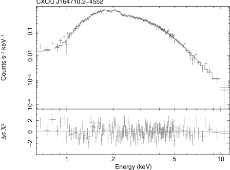
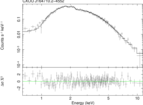
Figure 14: Left: Fit of the XMM-Newton EPIC-pn spectrum of CXOU J1647-4552  with an absorbed ntznoang model. Top: data and best fit model; bottom: residuals. Right: the same observation fitted with an absorbed ntzang model.

A systematic application of both models to magnetars spectra is in progress, and will be reported elsewhere (Israel et al. and Rea et al. in preparation). Here we present only an example which is illustrative of how the two atable spectral models behave when applied to X-ray data. Fig. 14 (left panel) shows the fit of the 0.1–10 keV XMM-Newton EPIC-pn spectrum of the transient AXP CXOU J1647-4552  taken on February 17 2007, i.e. about five months after a burst and a glitch were detected from this source (Krimm et al., 2006; Israel et al., 2006, see also Muno et al. 2007; Israel et al. 2007). All details about the observation will be reported in Israel et al. (in preparation). The spectrum has been modeled with the angle-integrated ntznoang model, modified by interstellar absorption (phabs model in XSPEC). Data and best fitting model are shown in Fig. 14 and the best fit parameters are listed in Table 1. As expected, and as it has been also found in other applications of the RCS model (Rea et al., 2008), the inferred value of the column density is smaller than that implied by a blackbody plus power-law fit. This is because the empirical blackbody plus power-law modelling is known to overestimate the soft X-ray emission and, in turn, the value of the interstellar absorption.

Since the fit is already very good ($\chi^{2}_{\nu}=0.81$), there is no statistical need to introduce two further parameters. However, we also tried to fit the same observation with an absorbed ntzang model, with the only goal to check and test the correctness of its XSPEC implementation; results are shown in Fig 14 (right panel) and reported in Table 1. As expected, the values of the angles are unconstrained, and the remaining parameters are in agreement with those found with the first model. Again, is not our main scope to provide the physical values of the angles here: instead we stress that this figure is presented purely as an illustration. Nevertheless, the successful spectral fit with the ntznoang model clearly demonstrates that the model can catch the main features of the magnetar emission and reproduce them quantitatively.

6 Discussion and conclusions

In this paper we have investigated how the thermal spectrum emitted by the star surface gets distorted by repeated resonant scatterings onto mildly relativistic magnetospheric electrons using a Monte Carlo technique. The goal of this study has been twofold. Our first motivation has been to create a model archive which could be implemented as a tabulated model in XSPEC and directly applied to fit the spectra of magnetar candidates. The model is available in two versions, with or without the explicit dependence on the two angles which give the inclination of the line-of-sight and the magnetic axis wrt the star spin. A systematic application to different sources is under way and here a (preliminary) fit to the XMM-Newton spectrum of CXOU J1647-4552 has been presented, mainly for illustrative purposes.

In building our Monte Carlo code we have followed an approach similar to that discussed in Fernandez & Thompson (2007). However, the two codes differ in many respects. A major difference is in the adopted description of the velocity distribution of the scattering particles. We have explicitly accounted for the collective (bulk) electron motion associated to the charge flow in the magnetosphere, superimposed to which we assume a 1D relativistic Maxwellian distribution which simulates the particle velocity spread. We also allow for a completely general description of the star surface thermal map and this makes it possible to assess the effects of a (spatially) localized emission (e.g. by a hot spot). Moreover, in our treatment seed photons are not taken to move only in the radial direction but are drawn from a prescribed angular distribution which can account for magnetic beaming effects.

As the present application to CXOU J1647-4552  shows (§5; see also Lyutikov & Gavriil, 2006; Rea et al., 2007a, 2008), spectral models based on resonant cyclotron up-scattering of thermal photons in the magnetosphere of magnetars prove quite successful in interpreting quantitatively the soft ($\sim 1$–10 keV) emission from AXPs and SGRs. Albeit the numerical computation presented here includes several important details about the microphysics and the magnetospheric properties and geometry, it relies on some simplifying assumptions which reflect our poor knowledge on some key issues of magnetar physics.

A prominent one is the nature of the plasma which fills the magnetosphere. Most investigations on RCS, including our, restricted to unidirectional flows, i.e. assumed that scattering occur onto electrons (a simple bi-directional flow was considered by Fernandez & Thompson, 2007). As discussed by Beloborodov & Thompson (2007), in a twisted magnetosphere charges, accelerated by the self-induction electric field, may produce $e^{\pm}$. Pairs definitely contribute to the scattering depth . The final spectral shape depends on which species populate the corona and on their spatial and velocity distribution. Our choice of modelling the $e^{-}$ current in terms of a bulk motion plus a velocity spread seems to be at least in qualitative agreement with the analysis presented by Beloborodov & Thompson (2007). We point out, however, that the assumption of a 1D thermal distribution for the particle velocity in the local rest frame is somehow arbitrary and no attempt has been made here to assess the effects of other possible (local) distributions. This has been done, in a few representative cases, by Fernandez & Thompson (2007), who did not include, however, the charge bulk motion. By comparing our results with their, one may conclude that, while the general effects induced by magnetospheric RCS on primary thermal photons (i.e. the formation of a “thermal-plus-power-law” spectrum) are not much sensitive to the assumed particle velocity distribution, the details of the spectral shape do.

A further caveat concerns the star temperature distribution and the primary spectrum. Our model archive has been generated assuming that the star radiates a blackbody from a uniformly heated surface. At present it is unclear if magnetars do possess an atmosphere. A possibility is that highly energetic electrons hitting the surface knock out protons which then sublimate giving rise to a “current induced” atmosphere (Beloborodov & Thompson, 2007). Departures from a blackbody primary spectrum due to reprocessing in a strongly magnetized atmosphere are, however, not expected to be dramatic (see e.g. Zane et al., 2001; Ho & Lai, 2001; Lai & Ho, 2003). On the other hand, the issue of the surface thermal map appears more serious since even passively cooling isolated neutron stars are known to have a non-uniform surface temperature (see e.g. Page, 1995; Zane & Turolla, 2006). In the case of a magnetar, returning currents impacting on the star surface produce localized heating (TLK). Moreover, starquakes, possibly triggered by the strain accumulated during the growth of the twist and connected to the glitching activity discovered in AXPs (see e.g. Dall’Osso et al., 2003), can further contribute to the injection of heat into limited portions of the crust. Transient AXPs might be powered in a similar way by the sudden release of energy into a localized area of the star surface, as observations of the TAXP XTE J1810-197 seem to indicate (Gotthelf & Halpern, 2007).

Although the twisted dipole model used here has the advantage of simplicity while catching the essential physical features, most probably it gives only an idealized representation of the magnetic field outside a magnetar. The twist may be confined at high magnetic latitudes (TLK), or, if global, it might involve magnetic configurations more complex than a dipole. Possible evidence for a twist which involves in the first place the field lines closer to the magnetic poles have been discussed by Woods et al. (2007) in connection with the period derivative evolution and its correlation with spectral hardness in SGR 1806-20 before and after the giant flare of December 27 2004.

Both Lyutikov & Gavriil (2006) and Fernandez & Thompson (2007) assumed that scattering is conservative in the electron rest frame. As discussed in §2.3 this choice is quite adequate if spectral modeling is restricted to the soft X-ray range and has been retained in the present work. However, the X-ray spectra of magnetar candidates are nowadays known to exhibit also a high energy ($\sim 20$–200 keV) component, which is completely non-thermal and is responsible for about half of the bolometric flux. Although different scenarios for the origin of the high energy emission from magnetars have been put forward, not necessary involving RCS (see §1), an intriguing possibility is that also the hard tail arises because of resonant upscattering in the magnetosphere (Baring & Harding, 2007). Given the much higher photon energies (in the 100 keV range) this necessary requires the presence of highly relativistic electrons (pairs), and, consequently, any attempt to model RCS under those conditions demands for a fully relativistic, QED treatment of the scattering cross sections. Although we presented here spectra extending up to 100 keV, they must be considered as trustworthy only until $\hbar\omega\ll m_{e}c^{2}/\gamma$, i.e. up to a few tens of keV. Above these energies electron recoil starts to become important and the spectrum is expected to break. The precise localization of the break would come only from a consistent treatment, and is particularly important to explain the COMPTEL upper limits observed in some magnetar sources (Kuiper et al., 2006; Rea et al., 2007b). Moreover, if hard tails are due to a secondary population of ultra-relativistic electrons confined close to the stellar surface (as proposed by Baring & Harding, 2007), resonant scattering would occur at much higher values of the magnetic field, $B>B_{QED}$, which makes the need of a completely QED treatment of the cross section even more necessary. Same holds for computations aimed at assessing the role of ions in shaping the spectra. As previously discussed see §2.2, positively charged ions are expected to populate the twisted magnetosphere, but whether these particles can effectively shape the X-ray spectra is mainly related to the role of those ions located close to the star surface. The inclusion of this effect, however, requires the knowledge of the full QED resonant cross section for protons/ions which at present has not been investigated in detail.

Future work needs to address this issue, among others. Clearly, in order to to include the relativistic treatment of the scattering process in the electron rest frame, having a tested, reliable Monte Carlo code which can be easily generalized is of fundamental importance and this has been our second motivation in undertaking this study. In order to extend our computation of resonant electron cyclotron scattering to the relativistic regime, we are already completing a detailed investigation of the QED resonant cross section. This will be then implemented in our Monte Carlo code and results will be presented in forthcoming papers (Nobili, Turolla & Zane in preparation).

Table 1: Best fit values of the spectral parameters.

Parameters	ntznoang	ntzang
$N_{H}$	1.76${}^{+0.06}_{-0.05}$	1.76${}^{+0.04}_{-0.01}$
$kT$	0.625${}^{+0.007}_{-0.008}$	0.63 ${}^{+0.07}_{-0.01}$
$\beta_{bulk}$	0.60 ${}^{+0.03}_{-0.02}$	0.65 ${}^{+0.26}_{-0.07}$
$\Delta\phi$	0.40${}^{+0.03}_{-0.32}$	0.47 ${}^{+0.03}_{-0.06}$
$\chi$	–	$2.1\pm 1.8$
$\xi$	–	$82^{+89}_{-56}$
Norm	0.081${}^{+0.003}_{-0.003}$	0.003${}^{+0.140}_{-0.000}$
Flux	6	6
$\chi^{2}_{\nu}$ (dof)	0.81 (145)	0.83 (143)

Errors in the parameters are at 1$\sigma$ confidence level, $N_{H}$ is in units of $10^{22}\,{\rm cm}^{-2}$, $kT$ is in keV, $\chi,\xi$ are in degrees and the observed flux (1–10 keV) is in units of $10^{-12}\ {\rm erg\,s\,cm}^{-2}$.

Figure 1: Left: Computed spectra for $B=10^{14}~{}G$, $kT=0.5$ keV, $kT_{e}=30$ keV, $\beta_{bulk}=0.3$, $\Delta\phi=1$ and different values of the sky colatitude $\Theta_{s}$: $27^{\circ}$ (long dashed), $64^{\circ}$ (dash-triple dotted), $90^{\circ}$ (dash-dotted), $116^{\circ}$ (short dashed) and $153^{\circ}$ (dotted). The solid line represents the seed blackbody and counts have been summed over $\Phi_{s}$. Here seed photons are assumed to be completely polarized in the ordinary mode. Right: Same, but for seed photons completely polarized in the extraordinary mode.

Figure 2: Top: Computed spectra for $B=10^{14}~{}G$, $kT=0.5$ keV, $kT_{e}=30$ keV, $\Delta\phi=1$ and different values of $\beta_{bulk}$: $0.3$ (dotted), $0.5$ (short dashed), $0.7$ (dash-dotted) and $0.9$ (dash-triple dotted). The solid line represents the seed blackbody and counts have been summed over $\Phi_{s}$. The two panels correspond to two different values of the magnetic colatitude: $\Theta_{s}=64^{\circ}$ (left) and $\Theta_{s}=116^{\circ}$ (right). Seed photons are assumed to be 100% polarized in the ordinary mode. Bottom: Same, but for seed photons 100% polarized in the extraordinary mode.

Figure 3: Top: Computed spectra for $B=10^{14}~{}G$, $kT=0.5$ keV, $\beta_{bulk}=0.3$, $\Delta\phi=1$ and different values of $kT_{e}$: 5 keV (dotted), 15 keV (short dashed), 30  keV (dash-dotted), 60  keV (dash-triple dotted) and 120 keV (long dashed). The solid line represents the seed blackbody and counts have been summed over $\Phi_{s}$. The two panels correspond to two different values of the magnetic colatitude: $\Theta_{s}=64^{\circ}$ (left) and $\Theta_{s}=116^{\circ}$ (right). Seed photons are assumed to be 100% polarized in the ordinary mode. Bottom: Same, but for seed photons 100% polarized in the extraordinary mode.

Figure 4: Top: Computed spectra for $B=10^{14}~{}G$, $kT=0.5$ keV, $kT_{e}=30$ keV, $\beta_{bulk}=0.3$ and different values of $\Delta\phi$: 0.3 (dotted), 0.5 (short dashed), 0.7 (dash-dotted), 0.9 (dash-triple dotted), 1.1 (long dashed) and $\Delta\phi=1.2$ (solid line, top). The solid line at the bottom represents the seed blackbody and counts have been summed over $\Phi_{s}$. The two panels correspond to two different values of the magnetic colatitude: $\Theta_{s}=64^{\circ}$ (left) and $\Theta_{s}=116^{\circ}$ (right). Seed photons are assumed to be 100% polarized in the ordinary mode. Bottom: Same, but for seed photons 100% polarized in the extraordinary mode.

Figure 5: Computed spectra for $B=10^{14}~{}G$, $\Delta\phi=2$; the star is an aligned rotator seen north pole-on. Solid line: $kT=0.1$ keV, $\beta_{bulk}=0.7$; dashed line: $kT=0.6$ keV, $\beta_{bulk}=0.6$. In both cases $kT_{e}$ is related to $\beta_{bulk}$ through eq. (23); seed photons are unpolarized.

Figure 6: Photon index versus $\Delta\phi$ for $B=10^{14}~{}G$ (triangles) and $B=10^{15}~{}G$ (diamonds). See text for details

Figure 7: Spectrum from a single emitting patch on the star surface. The LOS is at $\Theta_{s}=90^{\circ}$ and $\Phi_{s}=20^{\circ}$ (dotted line), $140^{\circ}$ (dashed line) and $220^{\circ}$ (dash-dotted line). The solid line represents the seed blackbody. Because photons are collected in a single patch on the sky, the counting statistics is low at the higher energies and the spectrum looks “noisy”.

Figure 8: Left: degree of polarization as a function of $\Delta\phi$ for $B=10^{14}$ G, $kT=0.5$ keV, $\beta_{bulk}=0.3$ and $kT_{e}=30$ keV. Right: Same, but as a function of $kT_{e}$ for $\Delta\phi=1$. In both panels different curves correspond to: seed photons 100% polarized in the ordinary (solid line), extraordinary mode (dotted line), and unpolarized (dashed line). See text for details.

Figure 9: Degree of polarization as a function of $\beta_{bulk}$ for $kT_{e}=30$ keV and $\Delta\phi=1$. Other parameters and line code as in fig. 8.

Figure 10: Right: Degree of polarization as a function of the magnetic colatitude $\Theta$ at which seed photons are emitted. Here $kT=0.5$ keV, $\beta_{bulk}=0.3$, $keT_{e}=30$ keV and $\Delta\phi=1$. Left panel: $B=10^{14}$ G; right panel: $B=10^{15}$ G. In both panels different curves correspond to: ordinary (solid line), extraordinary seed photons (dotted line) an unpolarized seed photons (dashed line). Photons have been integrated over the entire sky at infinity and over the azimuthal angle at the star surface.

Figure 11: Degree of polarization as a function of energy for different values of the LOS inclination, $\Theta_{s}=162^{\circ}$ (solid), $126^{\circ}$ (dotted), $90^{\circ}$ (dashed), $54^{\circ}$ (dash-dotted) and $18^{\circ}$ (dash-triple dotted). Left: 100% extraordinary polarized seed photons. Right: 100% ordinary polarized seed photons. As in Fig. 7, the low statistics is responsible for the noisy appearance of the plot at higher energies. The decrease in the polarization degree with energy is clearly visible notwithstanding.

Figure 12: Computed spectra for $B=10^{14}~{}G$, $kT=0.5$ keV, $kT_{e}=30$ keV, $\beta_{bulk}=0.3$, $\Delta\phi=1$, $\xi=45^{\circ}$ and five different values of the viewing angle $\chi$: $0.01^{\circ}$ (dotted), $45^{\circ}$ (short dashed), $90^{\circ}$ (dash-dotted), $135^{\circ}$ (dashed-triple dotted), and $180^{\circ}$ (long dashed). The solid line represents the seed blackbody. Here seed photons are assumed to be completely polarized in extraordinary mode.

Figure 13: Left: the lightcurves in the soft (0.5–2 keV, solid line) and hard X-ray band (2–6 keV, dashed line); the model parameters are $\chi=90^{\circ}$, $\xi=10^{\circ}$, $\Delta\phi=0.7$, $\beta_{bulk}=0.3$ and $kT=0.3\ {\rm keV}$. Right: same as in the left panel, but for $\xi=50^{\circ}$. See text for details.

References

- Baring & Harding (2007) Baring M. G., Harding A. K. 2007, Ap&SS, 308, 109
- Beloborodov & Thompson (2007) Beloborodov A. M., Thompson C. 2007, ApJ, 657, 967
- Campana et al. (2007) Campana S., Rea N., Israel G. L., Turolla R., Zane S. 2007, A&A, 63, 1047
- Chatterejee et al. (2000) Chatterjee P., Hernquist L., Narayan R. 2000, ApJ, 534, 373
- Dall’Osso et al. (2003) Dall’Osso S., Israel G. L., Stella L., Possenti A., Perozzi E. 2003, ApJ, 599, 485
- Daugherty & Harding (1986) Daugherty J. K., Harding A. K. 1986, ApJ, 309, 362
- Daugherty & Ventura (1978) Daugherty J. K., Ventura J. 1978, PRD, 18, 1053
- Esposito et al. (2007) Esposito P., et al. 2007, A&A, 476, 321
- Götz et al. (2006) Götz D., Mereghetti S., Tiengo A., Esposito P. 2006 A&A, 449, L31
- den Hartog et al. (2006) den Hartog P. R., Hermsen W., Kuiper L., Vink J., in’t Zand J. J. M., Collmar W. 2006, A&A, 451, 587
- Duncan & Thompson (1992) Duncan R., Thompson C. 1992, ApJ, 392, L9
- Fernandez & Thompson (2007) Fernandez R., Thompson C., 2007, ApJ, 660, 615
- Gavriil et al. (2002) Gavriil F. P., Kaspi, V. M., Woods, P. M. 2002, Nature, 419, 142
- Gotthelf & Halpern (2007) Gotthelf E. V., Halpern, J.P. 2007, Ap&SS, 308, 79
- Güver, Özel & Lyutikov (2006) Güver T., Özel F., Lyutikov M., 2006, preprint [arXiv:astro-ph/0611405 ]
- Güver, Özel & Göḡüş (2007) Güver T., Özel F., Göḡüş E. 2007, preprint [arXiv:0705.3982]
- Harding & Daugherty (1991) Harding A. K., Daugherty J. K., 1991, ApJ, 374, 687
- Herold (1979) Herold H. 1979, PRD, 19, 2868
- Ho & Lai (2001) Ho W. C. G., Lai D. 2001, MNRAS, 327, 1081
- Kaspi et al. (2003) Kaspi V. M., Gavriil F. P., Woods P. M., Jensen J. B., Roberts M. S. E., Chakrabarty D. 2003, ApJ, 588, L93
- (21) Kaspi V. M., Gavriil F. P. 2006, ATel 794
- Krimm et al. (2006) Krimm H., Barthelmy S., Campana S. 2006, GCN, 5581
- Kuiper et al. (2006) Kuiper L., Hermsen W., den Hartog P. R., Collmar W. 2006, ApJ, 645, 556
- Israel et al. (2006) Israel G. L., Dall’Osso S., Campana S., Muno, M. P., Stella L. 2006, ATel, 932
- Israel et al. (2007) Israel G. L., Campana S., Dall’Osso S., Muno M. P., Cummings J., Perna R., Stella L. 2007, ApJ, 664, 448
- Lai & Ho (2003) Lai D., Ho W. C. G. 2003, ApJ, 588, 962
- Lyutikov & Gavriil (2006) Lyutikov M., Gavriil F. P. 2006, MNRAS, 368, 690
- Medin & Lai (2007) Medin Z., Lai D. 2007, MNRAS, 382, 1833
- Mereghetti et al. (2005a) Mereghetti S., Götz D., Mirabel I. F., Hurley K. 2005, A&A, 433, L9
- Mereghetti et al. (2005b) Mereghetti S., et al. 2005, ApJ, 628, 938
- Mereghetti et al. (2006) Mereghetti S., et al. 2006, A&A, 450, 759
- Mészaros (1992) Mészaros P. 1992, High-Energy Radiation from Magnetized Neutron Stars, University of Chicago Press, Chicago, IL
- Molkov et al. (2005) Molkov S., Hurley K., Sunyaev R., Shtykovsky P., Revnivtsev M., Kouveliotou C. 2005, A&A, 433, L13
- Muno et al. (2007) Muno M. P., Gaensler B. M., Clark J. S., de Grijs R., Pooley D., Stevens I. R., Portegies Zwart S. F. 2007, MNRAS, 378, L44
- Page (1995) Page D. 1995, ApJ, 442, 273
- Perna et al. (2000) Perna R., Hernquist L., Narayan R. 2000, ApJ, 541, 344
- Rea et al. (2005) Rea N., Oosterbroek T., Zane S., Turolla R., Méndez M., Israel G. L., Stella L., Haberl F. 2005, MNRAS, 361, 710
- Rea et al. (2007a) Rea N., Zane S., Lyutikov M., Turolla R., 2007, Ap&SS, 308, 61
- Rea et al. (2007b) Rea N., Turolla R., Zane S., Tramacere A., Stella L., Israel G. L., Campana R. 2007, ApJ, 661, L65
- Rea et al. (2008) Rea N., Zane S., Turolla R., Lyutikov M., Götz D. 2008, ApJ, submitted
- Revnivtsev et al. (2004) Revnivtsev M. G., et al., 2004, Astron. Letts., 30, 382
- Thompson & Duncan (1993) Thompson C., Duncan R. C., 1993, ApJ, 408, 194
- Thompson, Lyutikov & Kulkarni (2002) Thompson C., Lyutikov M., Kulkarni S. R., 2002, ApJ, 274, 332 (TLK)
- Thompson & Belobodorov (2005) Thompson C., Beloborodov A. M., 2005, ApJ, 634, 565
- Van Adelsberg & Lai (2006) van Adelsberg M., Lai D. MNRAS, 2006, 373, 1495
- Van Paradijs et al. (1995) van Paradijs J., Taam R. E., van den Heuvel E. P. J. 1995, A&A, 299, L41
- Ventura (1979) Ventura J. 1979, PRD, 19, 1684
- Zane et al. (2000) Zane S., Turolla R., Treves A. 2000, ApJ, 537, 387
- Zane et al. (2001) Zane S., Turolla R., Stella L., Treves A. 2001, ApJ, 560, 384
- Zane & Turolla (2006) Zane S., Turolla R. 2006, MNRAS, 366, 727
- Woods et al. (2005) Woods P. M. et al. 2005, ApJ, 629, 985
- Woods & Thompson (2006) Woods P. M., Thompson C. 2006, in Lewin W. H. G., van der Klis M., eds., Compact Stellar X-ray Sources, Cambridge University Press, p. 547
- Woods et al. (2007) Woods P. M., Kouveliotou C., Finger M. H., Göḡüş E., Wilson C. A., Patel S. K., Hurley K., Swank J. H. 2007, ApJ, 654, 470