Scalar FCNC and rare top decays in a two Higgs doublet model ”for the top”

Abstract

In the so called two Higgs doublet model for the top-quark (T2HDM), first suggested by Das and Kao, the top quark receives a special status, which endows it with a naturally large mass, and also potentially gives rise to large flavor changing neutral currents (FCNC) only in the up-quark sector. In this paper we calculate the branching ratio (BR) for the rare decays $t\to ch$ and $h\to\bar{t}c$ ($h$ is a neutral Higgs) in the T2HDM, at tree level and at 1-loop when it exceeds the tree-level. We compare our results to predictions from other versions of 2HDM’s and find that the scalar FCNC in the T2HDM can play a significant role in these decays. In particular, the 1-loop mediated decays can be significantly enhanced in the T2HDM compared to the 2HDM of types I and II, in some instances reaching $BR\sim 10^{-4}$ which is within the detectable level at the LHC.

I Introduction

The Standard Model (SM) of elementary particles has been highly successful in describing the observed and measured phenomena. It contains, however, an unexplored sector, namely, the Higgs sector. The SM also has several problems, one of which is the fermion mass hierarchy problem, especially the top quark having a much larger mass than all other quarks.

In the T2HDM which was first suggested by Das and Kao Das as an extension to the SM, and which can be viewed as a low-energy parametrization of a more fundamental theory, the top quark receives a special status by a particular Yukawa structure which endows the top quark with a naturally large mass, while at the same time giving rise to potentially large FCNC couplings in the up-quark sector. Such new FCNC interactions in the up-quark sector may drive FCNC decays such as $t\to ch$ and $h\to\bar{t}c$ that we will consider in this paper.

Previous studies bejar ; t-ch LHC aguilar-saavedra have shown that the $BR\left(t\to ch\right)$, where $h=H^{0},h^{0},A^{0}$, could reach up to $\sim 10^{-4}$ in the 2HDM type II and in the MSSM, and about $\sim 10^{-6}$ in the 2HDM type I. In addition, the FCNC top decays $t\to c\gamma,~{}cg,~{}cZ$ can range between $10^{-4}-10^{-10}$ depending on the underlying Higgs sector. In order to give a feeling of the maximal values expected for the BR’s of FCNC top rare decays to gauge-bosons and scalars within different scalar models, we collect in table 1 some highlights of the results obtained in bejar and reported in the review t-ch LHC aguilar-saavedra . Namely, the expected FCNC rates within the SM and the 2HDM of types I,II and III. Note that the values are given with: $m_{t}=178$ GeV, $\overline{m_{b}}(m_{t})=2.74$ GeV and $m_{H^{0}}=115$ GeV. The branching ratio depends strongly on these parameters, especially on $m_{b}$. Note also that the corresponding BR’s for the decays into a $u$ quark instead of a $c$ quark are a factor $\left|V_{ub}/V_{cb}\right|^{2}\simeq 0.0088$ smaller in the SM and in the 2HDM of types I and II.

	SM	2HDM-I,II	2HDM-III $A^{A^{A}}$
$BR(t\to c\gamma)$	$\sim 5\times 10^{-14}$	$\lower 2.15277pt\hbox{$\>\buildrel<\over{\sim}\>$}10^{-9}$	$\lower 2.15277pt\hbox{$\>\buildrel<\over{\sim}\>$}10^{-6}$ $A^{A^{A}}$
$BR(t\to cg)$	$\sim 5\times 10^{-12}$	$\lower 2.15277pt\hbox{$\>\buildrel<\over{\sim}\>$}10^{-8}$	$\lower 2.15277pt\hbox{$\>\buildrel<\over{\sim}\>$}10^{-4}$ $A^{A^{A}}$
$BR(t\to cZ)$	$\sim 1\times 10^{-14}$	$\lower 2.15277pt\hbox{$\>\buildrel<\over{\sim}\>$}10^{-10}$	$\lower 2.15277pt\hbox{$\>\buildrel<\over{\sim}\>$}10^{-7}$ $A^{A^{A}}$
$BR(t\to ch)$	$\sim 6\times 10^{-15}$	$\lower 2.15277pt\hbox{$\>\buildrel<\over{\sim}\>$}10^{-5}$	$\lower 2.15277pt\hbox{$\>\buildrel<\over{\sim}\>$}10^{-3}$ (tree level) $A^{A^{A}}$

Table 1: Top quark rare decays into $c\gamma$, $cg$, $cZ$, $ch$, within various models: the SM, the 2HDM of type I, II and type III. Our results are consistent with t-ch LHC aguilar-saavedra ; t-ch SM ; h-tc SM arhrib .

The estimated LHC discovery limit for $t\to ch$ is $BR(t\to ch)\sim 5\times 10^{-5}$ t-ch LHC aguilar-saavedra for an integrated luminosity of $100~{}fb^{-1}$. In the SM, this decay has a vanishingly small branching ratio $BR_{SM}(t\to cH^{0})\sim 6\times 10^{-15}$ t-ch LHC aguilar-saavedra ; t-ch SM ; h-tc SM arhrib , which is not accessible at the upcoming Large Hadron Collider (LHC). Thus the rare FCNC decays $t\to ch$ and $h\to\bar{t}c$ are extremely sensitive probes of new physics in the scalar sector.

In this work we will explore these rare decay channels, $t\to ch$ and $h\to\bar{t}c$, within the parameter space of the T2HDM, at the 1-loop level and, when allowed, also at the tree-level. We will focus on regions of the parameter space in which the $BR\left(t\to ch\right)$ can exceed the detection limit of the LHC, and also on regions where the $BR\left(t\to ch\right)$ and $BR\left(h\to\bar{t}c\right)$ can be enhanced significantly compared to other 2HDM.

The paper is organized as follows: in sections II and III we describe the main features of the T2HDM relevant for our analysis and in section IV we shortly discuss the constraints on the parameter space of the model. In section V we outline our analytical derivation and in section VI we give our numerical results. In section VII we summarize. In Appendix A we list the required Feynman rules, in Appendix B we give the 1-loop amplitudes, in Appendix C we define the 1-loop integrals and in Appendix D we derive the total Higgs width in the models considered.

II The two higgs doublets model “for the top”

In the T2HDM the second Higgs field couples only to the top-quark, while the first Higgs field couples to all other quarks Das :

$$\mathcal{L}_{Y}= -\bar{Q}_{Li}\Phi_{1}F_{ij}d_{Rj}-\bar{Q}_{Li}\tilde{\Phi}_{1}G_{ij=1,2}\left(\begin{array}[]{c}u\\ c\end{array}\right)_{R}$$ (3)

$$-\bar{Q}_{Li}\tilde{\Phi}_{2}G_{i3}t_{R}+h.c.\mbox{ ,}$$ (4)

where: $i,j=1,2,3$ are flavor indices, $L(R)\equiv\left(1-(+)\gamma^{5}\right)/2$ are the chiral left (right) projection operators, $f_{L(R)}=L(R)f$ are left(right)-handed fermion fields, $Q_{L}$ is the left-handed $SU(2)$ quark doublet and $F,G$ are general $3\times 3$ Yukawa matrices in flavor space. Also, $\Phi_{1,2}$ are the Higgs doublets:

$$\Phi =\left(\begin{array}[]{c}\Phi^{+}\\ \frac{v+\Phi^{0}}{\sqrt{2}}\end{array}\right),\quad\tilde{\Phi}=\left(\begin{array}[]{c}\frac{v^{*}+\Phi^{0*}}{\sqrt{2}}\\ -\Phi^{-}\end{array}\right).$$

The Yukawa texture of (4) can be realized in terms of a $Z_{2}$-symmetry under which the fields transform as follows Das :

$$\Phi_{1}\to-\Phi_{1}, \quad d_{R}\to-d_{R},\quad u_{R}\to-u_{R}\;(u=u,c),$$ (5)

$$\Phi_{2}\to+\Phi_{2}, \quad Q_{L}\to+Q_{L},\quad t_{R}\to+t_{R}.$$

The Higgs potential is a general 2HDM one HHG :

$$\mathcal{L}_{H}= \lambda_{1}\left(\Phi_{1}^{+}\Phi_{1}-v_{1}^{2}/2\right)^{2}+\lambda_{2}\left(\Phi_{2}^{+}\Phi_{2}-v_{2}^{2}/2\right)^{2}$$

$$+\lambda_{3}\left[\left(\Phi_{1}^{+}\Phi_{1}-v_{1}^{2}/2\right)+\left(\Phi_{2}^{+}\Phi_{2}-v_{2}^{2}/2\right)\right]^{2}$$

$$+\lambda_{4}\left[\left(\Phi_{1}^{+}\Phi_{1}\right)\left(\Phi_{2}^{+}\Phi_{2}\right)-\left(\Phi_{1}^{+}\Phi_{2}\right)\left(\Phi_{2}^{+}\Phi_{1}\right)\right]$$

$$+\lambda_{5}\left|\Phi_{1}^{+}\Phi_{2}-v_{1}v_{2}/2\right|^{2}.$$ (6)

where we have included the term $\propto\lambda_{5}$ which softly breaks the $Z_{2}$-symmetry in (5) and which can also give rise to CP-violation georgi soft CP and Z2 .

The top-quark acquires a mass term primarily from the second Higgs vacuum expectation value (VEV), which we will choose to be much larger than the first Higgs VEV:

$$\tan\beta\equiv\frac{v_{2}}{v_{1}} \gg 1~{}.$$ (7)

Eq. 7 above is the working assumption of the T2HDM.

The particular Yukawa structure of (4) gives rise to various other interesting features of the T2HDM:

• Enhanced $H^{+}\bar{c}b$ coupling: The $H^{+}\bar{c}b$ interaction term is naively enhanced by a factor of $V_{tb}/V_{cb}$ compared to other 2HDM’s, where $V$ is the CKM matrix. This property which motivated the analysis in soni 15 Z-bs ; soni 21 most calcs , also motivated the present work since, as we shall later see, the 1-loop FCNC decays $t\to ch$ and $h\to\bar{t}c$ are expected to be enhanced, due to this large $H^{+}cb$ coupling, naively by this factor compared to e.g., the 2HDM of type II.

• Tree-level FCNC couplings in the up-quark sector: While there are no tree-level FCNC interactions in the down-quark sector (as for the example in the case of the type III 2HDM atwood reina soni bound neutral ), there are a-priori ${\cal O}(1)$ FCNC $htc$ and $htu$ couplings.

• Enhanced couplings to up quarks: The couplings of the three neutral scalars ($h\equiv H^{0},~{}h^{0},~{}or~{}A^{0}$) to all the quarks except for the top quark, increase with $\tan\beta$. For example, the $hcc$ coupling is $\propto m_{c}\tan\beta$ in the T2HDM as opposed to being $\propto m_{c}/\tan\beta$ in e.g., the type II 2HDM which also underlies the MSSM. Since $\tan\beta>>1$ is the working assumption of the T2HDM, one expects a large enhancement of the $hcc$ coupling in the T2HDM. This motivated the work in soni 13 3jet .

III Yukawa interactions and the Theoretical setup

A detailed derivation of all Yukawa interactions in the physical mass basis can be found in thesis (see also soni 34 best ). We use the results of thesis , which are also summarized as a list of scalar-quark-quark Feynman rules in Appendix A.

Below we highlight only the new Yukawa interactions that will be the focus of our analysis. In particular, as mentioned above, in the T2HDM the $H^{+}\bar{c}b$ interaction is different from the typical 2HDM scenario:

$$\mathcal{L}_{H^{+}cb} =\frac{g}{\sqrt{2}m_{W}}H^{+}\bar{c}\left[\tan\beta VM_{d}R+\left(-M_{u}\tan\beta+\Sigma^{\dagger}\left(\tan\beta+\cot\beta\right)\right)VL\right]_{cb}b$$

$$\sim\frac{g}{\sqrt{2}m_{W}}H^{+}\bar{c}\left[\tan\beta V_{cb}m_{b}R+m_{c}\left(-\tan\beta V_{cb}+\xi^{*}\left(\tan\beta+\cot\beta\right)V_{tb}\right)L\right]b\mbox{ ,}$$ (8)

where  $M_{d}=diag(m_{d},m_{s},m_{b})$, $M_{u}=diag(m_{u},m_{c},m_{t})$ and $\Sigma$ is a new mixing matrix in the up-quark sector that can be parametrized as thesis :

$$\frac{\Sigma}{m_{t}} =\left(\begin{array}[]{ccc}\frac{m_{u}}{m_{t}}\epsilon_{ct}^{2}\left|\xi^{\prime}\right|^{2}\left(1-\left|\epsilon_{ct}\xi\right|^{2}\right)&\frac{m_{u}}{m_{t}}\epsilon_{ct}^{2}\xi^{\prime*}\xi\sqrt{1-\left|\epsilon_{ct}\xi\right|^{2}}&\frac{m_{u}}{m_{t}}\epsilon_{ct}\xi^{\prime*}\left(1-\left|\epsilon_{ct}\xi\right|^{2}\right)\sqrt{1-\left|\epsilon_{ct}\xi^{\prime}\right|^{2}}\\ \epsilon_{ct}^{3}\xi^{*}\xi^{\prime}\sqrt{1-\left|\epsilon_{ct}\xi\right|^{2}}&\epsilon_{ct}^{3}\left|\xi\right|^{2}&\epsilon_{ct}^{2}\xi^{*}\sqrt{1-\left|\epsilon_{ct}\xi\right|^{2}}\sqrt{1-\left|\epsilon_{ct}\xi^{\prime}\right|^{2}}\\ \epsilon_{ct}\xi^{\prime}\left(1-\left|\epsilon_{ct}\xi\right|^{2}\right)\sqrt{1-\left|\epsilon_{ct}\xi^{\prime}\right|^{2}}&\;\epsilon_{ct}\xi\sqrt{1-\left|\epsilon_{ct}\xi\right|^{2}}\sqrt{1-\left|\epsilon_{ct}\xi^{\prime}\right|^{2}}&\left(1-\left|\epsilon_{ct}\xi\right|^{2}\right)\left(1-\left|\epsilon_{ct}\xi^{\prime}\right|^{2}\right)\end{array}\right),$$ (12)

where $\epsilon_{ct}\equiv m_{c}/m_{t}$ and $\xi,\xi^{\prime}$ are dimensionless parameters naturally of ${\cal O}(1)$.

As we can see from (8), the $H^{+}\bar{c}b$ vertex has terms proportional to $V_{cb}$ which are common to other 2HDM’s, but has an additional term which is not CKM suppressed and is proportional to $\left(\tan\beta+\cot\beta\right)\times\left(\Sigma^{\dagger}V\right)_{cb}\sim m_{c}\xi^{*}\tan\beta V_{tb}$. As we shall see below, this apparent enhancement to $H^{+}\bar{c}b$ coupling will drive the main contribution to the 1-loop diagrams with internal $H^{+}$ and $b$.

The $H^{+}\bar{t}b$ vertex also receives an additional term within the T2HDM:

$$\mathcal{L}_{H^{+}tb}\sim \frac{g}{\sqrt{2}m_{W}}H^{+}\bar{t}\left\{\tan\beta V_{tb}m_{b}R+\left[m_{t}V_{tb}\cot\beta\vphantom{\left|\xi\right|^{2}}\right.\right.$$

$$\left.\left.-m_{t}V_{tb}\epsilon_{ct}^{2}\left(\left|\xi\right|^{2}+\left|\xi^{\prime}\right|^{2}\right)\left(\tan\beta+\cot\beta\right)\right]L\right\}b.$$ (13)

We see, however, that this new contribution to the $H^{+}tb$ coupling is sub-leading and vanishes in the limit $\xi,\xi^{\prime}\to 0$, in which case the $H^{+}\bar{t}b$ interaction in (13) converges to that of a 2HDM types I and II.

As for the neutral Higgs sector, there is no a priori distinction between $h^{0}$ and $H^{0}$ other than the rotation angle $\alpha$. In particular, the $h^{0}tc$ and $H^{0}tc$ Yukawa interactions are:

$$\mathcal{L}_{h^{0}tc} \sim h^{0}\bar{t}\left[-\frac{g}{2m_{W}}\left(\frac{\cos\alpha}{\sin\beta}+\frac{\sin\alpha}{\cos\beta}\right)m_{c}\xi\left(R+\epsilon_{ct}L\right)\right]c~{},$$ (14)

$$\mathcal{L}_{H^{0}tc} \sim H^{0}\bar{t}\left[\frac{g}{2m_{W}}\left(-\frac{\sin\alpha}{\sin\beta}+\frac{\cos\alpha}{\cos\beta}\right)m_{c}\xi\left(R+\epsilon_{ct}L\right)\right]c~{},$$ (15)

where we have used the off-diagonal terms of $\Sigma$ from Eq. 12, neglecting terms of order $\epsilon_{ct}^{2}$ (recall $\epsilon_{ct}=m_{c}/m_{t}$) for which $\Sigma_{tc}\sim m_{c}\xi$ and $\left(\Sigma^{\dagger}\right)_{tc}\sim m_{c}\epsilon_{ct}\xi$.

For arbitrary $\alpha$ and $\beta$, the above FCNC interactions will lead to both $t\to cH^{0}$ and $t\to ch^{0}$ (or $H^{0}\to\bar{t}c$ and $h^{0}\to\bar{t}c$ if $m_{t}<m_{H^{0}},m_{h^{0}}$) decays at tree level. One can, however, eliminate one of the two tree-level $h^{0}tc$ or $H^{0}tc$ couplings by choosing a specific direction with respect to the mixing angles $\alpha$ and $\beta$ of the neutral Higgs sector. For example, the tree-level $H^{0}\bar{t}c$ coupling can be eliminated if one of the following two conditions is satisfied:

1. $\xi=0$.

2. $-\frac{\sin\alpha}{\sin\beta}+\frac{\cos\alpha}{\cos\beta}=0$ implying $\alpha=\beta+n\pi$.

Without loss of generality, let us consider the case in which either the $h^{0}tc$ or the $H^{0}tc$ coupling vanishes at tree-level. For definiteness, we will adopt the second choice above, $\alpha=\beta$, which sets:

$$\mathcal{L}^{\alpha=\beta}_{H^{0}tc}=0~{},$$ (16)

and gives:

$$\mathcal{L}^{\alpha=\beta}_{h^{0}tc} \sim h^{0}\bar{t}\left[-\frac{gm_{c}\xi}{2m_{W}}\left(\tan\beta+\cot\beta\right)\left(R+\epsilon_{ct}L\right)\right]c~{}.$$ (17)

There are several reasons which motivate an analysis of the case $\alpha=\beta$ rather than the case of generic mixing angles and for preferring this choice over the choice $\xi=0$ which also eliminates the tree-level $H^{0}tc$ coupling:

1. $\xi=0$ is disfavored by the analysis in soni 34 best , as we will recapitulate in Sec. IV.

2. $\xi=0$ diminishes the potentially enhanced term in the $H^{+}\bar{c}b$ coupling, as is evident from Eq. 8.

3. The limit $\alpha=\beta$ is a natural result of the MSSM, when the mass of the CP-odd neutral Higgs, $A^{0}$, is large (see e.g. HHG in the limit $m_{A^{0}}\to\infty$). The choice $\alpha=\beta$ is widely used in the literature, partly for this reason. Thus, even though the T2HDM setup is not natural within the MSSM, this will help us compare our results with other existing results in different types of 2HDM’s.

4. The limit $\alpha=\beta$ sets the scalar $H^{0}$ to be SM-like, in which case the direct bounds on the SM Higgs mass roughly apply to $H^{0}$. Also, $H^{0}$ will have SM-like Yukawa couplings to quarks:

   $$\mathcal{L}_{Y_{H^{0}}}^{\alpha=\beta} \supset H^{0}\bar{d}\left[-\frac{gM_{d}}{2m_{W}}\right]d+H^{0}\bar{u}\left[-\frac{gM_{u}}{2m_{W}}\right]u.$$ (18)

Finally, the $h^{0}\bar{t}t$ interaction, with $\alpha=\beta$, reads:

$$\mathcal{L}\sim h^{0}\bar{t}\left\{\frac{gm_{t}}{2m_{W}}\left[-\cot\beta+\epsilon^{2}_{ct}\left(\left|\xi\right|^{2}+\left|\xi^{\prime}\right|^{2}\right)\left(\tan\beta+\cot\beta\right)\right]R\right.$$

$$\left.+\left(h.c.\right)L\vphantom{\frac{a}{b}}\right\}t~{},$$ (19)

where $\Sigma_{tt}=\left(\Sigma^{\dagger}\right)_{tt}\sim m_{t}-m_{c}\epsilon_{ct}\left(\left|\xi\right|^{2}+\left|\xi^{\prime}\right|^{2}\right)$. As in the case of $H^{+}\bar{t}b$, the term $\propto m_{t}\tan\beta$ cancels, and we are left with the usual $m_{t}/\tan\beta$ term plus terms that are suppressed either by $\epsilon_{ct}^{2}$ or $\cot^{2}\beta$.

IV The parameter space of the T2HDM

The parameter space of the T2HDM was recently analyzed in soni 34 best . Here we recapitulate the bounds on the parameter space of T2HDM that were derived in soni 34 best by performing a best fit to several experimentally measured observables mainly associated with B-decays. The processes that were selected were the ones that are potentially most sensitive to the charged sector of the T2HDM. The analysis in soni 34 best is directly relevant to the present work, and so we list below the final results of soni 34 best (recall that $\xi=\left|\xi\right|e^{i\varphi_{\xi}}$):

$$m_{H^{\pm}} = \left(660_{-280}^{+390}\right)\mbox{ GeV},$$

$$\tan\beta = 28_{-8}^{+44},$$

$$0.5< \left|\xi\right| <1,$$

$$\varphi_{\xi} = \left(110_{-65}^{+30}\right)^{\circ},$$

$$\left|\xi^{\prime}\right| \sim 0.21,$$

$$\varphi_{\xi^{\prime}} \sim 250^{\circ}.$$ (20)

Note that:

• These values for $\tan\beta$ and $m_{H^{+}}$ are allowed also within the framework of a type II 2HDM arhrib .

• The authors of soni 34 best didn’t consider possible constraints on the FCNC $H^{0}$ - up-quark couplings of the T2HDM, coming from the recently measured $D^{0}$ oscillations. We note, however, that such contributions to the $D^{0}-\bar{D}^{0}$ mass difference is suppressed by a factor of $\left(\frac{1}{\tan\beta}\frac{m_{c}}{m_{t}}\frac{m_{H^{+}}}{m_{h^{0}}}\right)^{2}$ compared to the charged Higgs contribution that was considered in soni 34 best , and therefore does not impose further constraints on the FCNC parameter space of the neutral sector other than those found in atwood reina soni bound neutral ; soni 21 most calcs .

There are also direct constraints on the neutral Higgs masses from high-energy collider experiments PDG :

• The direct bound on the SM Higgs (which also applies to $H^{0}$ of the T2HDM when $\alpha=\beta$) is: $m_{H^{0}}>114$ GeV.

• The bounds on the mass of lightest neutral scalar and the charged scalar in supersymmetry are: $m_{h}>90$ GeV and $m_{H^{+}}>80$ GeV.

V Analytical Results

V.1 The tree-level $t\to ch^{0}$ or $h^{0}\to\bar{t}c$

As stated above, when $\alpha=\beta$ the decays $t\to ch^{0}$ or $h^{0}\to\bar{t}c$ can proceed at tree-level (when kinematically allowed) while the corresponding decays involving $H^{0}$ are mediated at 1-loop. Using the tree-level coupling $h^{0}\bar{t}c$ in Eq. 17, the tree-level amplitude for the process $t\to ch^{0}$ is:

$$\mathcal{M}\left(t\to ch^{0}\right)= \bar{u}_{c}\left[\frac{g}{2m_{W}}\left(\left(M_{u}\right)_{ct}\frac{\sin\alpha}{\cos\beta}\right.\right.$$ (21)

$$\left.\left.-\Sigma_{ct}\left(\frac{\cos\alpha}{\sin\beta}+\frac{\sin\alpha}{\cos\beta}\right)\right)R+\left(h.c.\right)L\right]u_{t},$$

where from (12) we have:

$$\Sigma_{ct} =m_{t}\epsilon_{ct}^{2}\xi^{*}\sqrt{1-\left|\epsilon_{ct}\xi\right|^{2}}\sqrt{1-\left|\epsilon_{ct}\xi^{\prime}\right|^{2}}\sim m_{c}\epsilon_{ct}\xi^{*},$$

$$\left(\Sigma^{\dagger}\right)_{ct} =m_{t}\epsilon_{ct}\xi^{*}\sqrt{1-\left|\epsilon_{ct}\xi\right|^{2}}\sqrt{1-\left|\epsilon_{ct}\xi^{\prime}\right|^{2}}\sim m_{c}\xi^{*}.$$ (22)

Taking $\alpha=\beta$ we then obtain:

$$\mathcal{M}\left(t\to ch^{0}\right) =\bar{u}_{c}\frac{-g}{2m_{W}}\left(\cot\beta+\tan\beta\right)m_{c}\xi^{*}\left[\epsilon_{ct}R+L\right]u_{t}$$

$$\equiv\bar{u}_{c}\left[M_{R}R+M_{L}L\right]u_{t}.$$ (23)

The squared amplitude, summed over initial and final state polarizations is then:

$$\underset{pol}{\sum}\left|\mathcal{M}\right|^{2} = 2m_{c}m_{t}\left(M_{L}M_{R}^{*}+M_{R}M_{L}^{*}\right)$$ (24)

$$+\left(m_{t}^{2}+m_{c}^{2}-m_{h}^{2}\right)\left(M_{L}M_{L}^{*}+M_{R}M_{R}^{*}\right)$$

$$= \frac{g^{2}m_{c}^{2}}{4m_{W}^{2}}\left(\cot\beta+\tan\beta\right)^{2}\left|\xi\right|^{2}$$

$$\times\left[2m_{c}m_{t}\cdot 2\epsilon_{ct}+\left(m_{t}^{2}+m_{c}^{2}-m_{h^{0}}^{2}\right)\left(1+\epsilon_{ct}^{2}\right)\right]$$

$$\sim \frac{g^{2}m_{c}^{2}}{4m_{W}^{2}}\tan^{2}\beta\left|\xi\right|^{2}\left[m_{t}^{2}-m_{h^{0}}^{2}\right]~{}.$$

where we have neglected terms of ${\cal O}(m_{c}^{2}/m_{t}^{2})$ and of ${\cal O}(\cot\beta)$ in accordance with the working assumption of the T2HDM, i.e., that $\tan\beta>>1$. The width of $t\to ch^{0}$ then reads:

$$\Gamma\left(t\to ch^{0}\right) =4\pi\cdot\lambda^{\frac{1}{2}}\left(1,\frac{m_{c}^{2}}{m_{t}^{2}},\frac{m_{h^{0}}^{2}}{m_{t}^{2}}\right)\cdot\frac{\underset{pol}{\sum}\overline{\left|\mathcal{M}\right|^{2}}}{64\pi^{2}m_{t}}$$

$$\sim\frac{g^{2}\left|\xi\right|^{2}m_{t}m_{c}^{2}}{128\pi m_{W}^{2}}\tan^{2}\beta\left(1-\frac{m_{h^{0}}^{2}}{m_{t}^{2}}\right)^{2},$$ (25)

where $\lambda\left(x,y,z\right)=x^{2}+y^{2}+z^{2}-2xy-2xz-2yz$ and $\underset{pol}{\sum}\overline{\left|\mathcal{M}\right|^{2}}=\frac{1}{2}\underset{pol}{\sum}\left|\mathcal{M}\right|^{2}$ is the squared amplitude summed over final polarizations and averaged over the initial top polarizations.

We then obtain the following $BR\left(t\to ch^{0}\right)$ (for large $\tan\beta$):

$$BR\left(t\to ch^{0}\right)\sim \frac{\left|\xi\right|^{2}m_{c}^{2}}{2m_{W}^{2}}\tan^{2}\beta\left(1-\frac{m_{h^{0}}^{2}}{m_{t}^{2}}\right)^{2}\left(1-\frac{m_{W}^{2}}{m_{t}^{2}}\right)^{-1}$$

$$\times\left(1-2\frac{m_{W}^{2}}{m_{t}^{2}}+\frac{m_{t}^{2}}{m_{W}^{2}}\right)^{-1},$$ (26)

where for the total top-quark decay width ($\Gamma_{t}$) we took (at tree-level and neglecting terms of order $m_{b}^{2}/m_{t}^{2}$ PDG ):

$$\Gamma_{t} =\Gamma\left(t\to bW^{+}\right)$$

$$\sim\frac{g^{2}m_{t}}{64\pi}\left(1-\frac{m_{W}^{2}}{m_{t}^{2}}\right)\left(1-2\frac{m_{W}^{2}}{m_{t}^{2}}+\frac{m_{t}^{2}}{m_{W}^{2}}\right)~{}.$$ (27)

For instance, taking $\tan\beta=28$, $\left|\xi\right|=0.8$ (compatible with the bounds in (20)) and $m_{h^{0}}=91$ GeV, we get (when $\Gamma_{t}=\Gamma(t\to bW^{+})$):

$$BR\left(t\to ch^{0}\right)\sim 0.0077~{}.$$ (28)

Note that if $m_{H^{+}}<m_{t}$, then the top can also have an appreciable BR to $t\to H^{+}b$ which must be taken into account in $\Gamma_{t}$.

The decay width for the reverse $h^{0}\to\bar{t}c$ process (corresponding to the case $m_{h^{0}}>m_{t}$) can be obtained by applying a crossing symmetry to the squared amplitude of the decay $t\to ch^{0}$ in Eq. 24 (see e.g., peskin ):

$$\underset{pol}{\sum}\left|\mathcal{M}\right|^{2}(h^{0} \to\bar{t}c)=\underset{pol}{\sum}\left|\mathcal{M}\right|^{2}(t\to ch^{0})$$

$$\sim\frac{g^{2}m_{c}^{2}}{4m_{W}^{2}}\tan^{2}\beta\left|\xi\right|^{2}\left[m_{h^{0}}^{2}-m_{t}^{2}\right]~{},$$ (29)

from which we get:

$$\Gamma(h \to\bar{t}c+\bar{c}t)=2\times\Gamma\left(h^{0}\to\bar{t}c\right)$$

$$=2N_{c}\lambda^{\frac{1}{2}}\left(1,\frac{m_{c}^{2}}{m_{h^{0}}^{2}},\frac{m_{t}^{2}}{m_{h^{0}}^{2}}\right)\cdot\frac{\underset{pol}{\sum}\overline{\left|\mathcal{M}\right|^{2}}(h^{0}\to tc)}{16\pi m_{h^{0}}}$$

$$\sim\frac{N_{c}\left|\xi\right|^{2}g^{2}m_{h^{0}}m_{c}^{2}}{32\pi m_{W}^{2}}\tan^{2}\beta\left(1-\frac{m_{t}^{2}}{m_{h^{0}}^{2}}\right)^{2},$$ (30)

where $N_{c}=3$ is a color factor, and $\underset{pol}{\sum}\overline{\left|\mathcal{M}\right|^{2}}=\underset{pol}{\sum}\left|\mathcal{M}\right|^{2}$, since the initial state is a scalar field.

To get an estimate of the $BR(h^{0}\to\bar{t}c)$ we need the total width of $h^{0}$. For $\alpha=\beta$ and assuming also that $m_{h^{0}}<2m_{A^{0}},2m_{H^{+}}$, the total decay width of $h^{0}$ is mainly comprised of fermion decays, since the couplings $W^{+}W^{-}h^{0}$, $Z^{0}Z^{0}h^{0}$ and $H^{0}H^{0}h^{0}$ are all $\propto\sin\left(\beta-\alpha\right)$ (see table 7 and App. D). Thus, below the $t\bar{t}$ threshold (at about $m_{h^{0}}\lower 2.15277pt\hbox{$\>\buildrel<\over{\sim}\>$}340$ GeV) the decay $h^{0}\to b\bar{b}$ dominates, with (see App. D):

$$\Gamma\left(h^{0}\to\bar{b}b\right) \sim\frac{N_{c}g^{2}m_{b}^{2}m_{h^{0}}}{32\pi m_{W}^{2}}\tan^{2}\beta~{}.$$ (31)

In this case, we obtain:

$$BR\left(h^{0}\to\bar{t}c+\bar{c}t\right) \sim\left|\xi\right|^{2}\frac{m_{c}^{2}}{m_{b}^{2}}\left(1-\frac{m_{t}^{2}}{m_{h^{0}}^{2}}\right)^{2},$$ (32)

which for e.g., $\left|\xi\right|=0.8$ and $m_{h^{0}}=300$ GeV, amounts to $BR\left(h^{0}\to\bar{t}c+\bar{c}t\right)\sim 0.023$.

V.2 The 1-loop decays $t\to cH^{0}$ or $H^{0}\to\bar{t}c$

The 1-loop $t\to cH^{0}$ decay amplitude is composed of 10 Feynman diagrams which are shown in Fig. 1. The individual amplitudes corresponding to each of the 10 diagrams are given in App. B. The calculation was performed in the t’Hooft Feynman gauge and was aimed to be as model-independent as possible, therefore assuming general vertices for the general fields $q_{i}$, $V_{\alpha}$ and $H_{\alpha}$ which stand for a quark (up or down type), vector (gauge) fields and scalar fields, respectively (see the calculation setup as defined by Fig. 13 in App. B). This allowed us to easily calculate the partial width for $t\to cH^{0}$ (or for $H^{0}\to\bar{t}c$) in different multi-Higgs models, by inserting the appropriate vertices and fields.

The 1-loop integrals were evaluated numerically with FORTRAN (f77) using the FF package ff vanold . The calculations were done using the Passarino-Veltman reduction scheme, which expresses the integrals in terms of basic scalar n-point functions. In particular, the vector and tensor integrals were computed using linear combinations of the scalar functions (for explicit formulae see e.g. App. A in bejar ). In App. C we describe the reduction scheme used to calculate the 1-loop integrals.

Figure 1: 1-loop Feynman diagrams for $t\to cH^{0}$

As in the tree-level case, let us define the total amplitude as:

$$\mathcal{M} = \frac{i\bar{u}_{c}}{16\pi^{2}}\left(M_{L}L+M_{R}R\right)u_{t}~{},$$ (33)

where

$$M_{L,R}\equiv\sum_{i=1-10}M^{i}_{L,R}~{},$$ (34)

and $M^{i}_{L,R}$ are parts of the amplitude corresponding to diagram $i$ which are given in App. B.

Using Eq. 33 we can write the squared amplitude summed over polarizations as:

$$\underset{pol}{\sum}\left|\mathcal{M}\right|^{2}= \frac{1}{2}\frac{1}{256\pi^{4}}\left[2m_{c}m_{t}\left(M_{L}M_{R}^{*}+M_{R}M_{L}^{*}\right)\right.$$

$$\left.+\left(m_{c}^{2}+m_{t}^{2}-m_{h}^{2}\right)\left(M_{L}M_{L}^{*}+M_{R}M_{R}^{*}\right)\right],$$ (35)

from which we obtain:

$$\Gamma=4\pi\cdot\lambda^{\frac{1}{2}}\left(1,\frac{m_{c}^{2}}{m_{t}^{2}},\frac{m_{H}^{2}}{m_{t}^{2}}\right)\cdot\frac{\underset{pol}{\sum}\overline{\left|\mathcal{M}\right|^{2}}}{64\pi^{2}m_{t}},$$ (36)

where: $\underset{pol}{\sum}\overline{\left|\mathcal{M}\right|^{2}}=\frac{1}{2}\underset{pol}{\sum}\left|\mathcal{M}\right|^{2}$.

Finally, the BR for the decay $t\to cH^{0}$ is:

$$BR\left(t\to cH^{0}\right)\sim\frac{\Gamma\left(t\to cH^{0}\right)}{\Gamma\left(t\to bW^{+}\right)}\mbox{ ,}$$ (37)

where $\Gamma(t\to bW^{+})$ is given in Eq. 27. As before, if $m_{H^{+}}<m_{t}$, then the top can also have an appreciable BR to $t\to H^{+}b$ which must be taken into account for the total top width.

For the case $m_{H^{0}}>m_{t}$ we again consider the reversed 1-loop decay $H^{0}\to\bar{t}c+\bar{c}t$, where

$$\Gamma\left(H^{0}\to\bar{t}c+\bar{c}t\right)=2\times\Gamma\left(H^{0}\to\bar{t}c\right)$$

$$=2N_{c}\lambda^{\frac{1}{2}}\left(1,\frac{m_{c}^{2}}{m_{H^{0}}^{2}},\frac{m_{t}^{2}}{m_{H^{0}}^{2}}\right)\cdot\frac{\underset{pol}{\sum}\overline{\left|\mathcal{M}\right|^{2}}(H^{0}\to tc)}{16\pi m_{H^{0}}},$$ (38)

where, as in the tree-level case, $\underset{pol}{\sum}\overline{\left|\mathcal{M}\right|^{2}}(H^{0}\to\bar{t}c)=\underset{pol}{\sum}\left|\mathcal{M}\right|^{2}(H^{0}\to\bar{t}c)=\underset{pol}{\sum}\left|\mathcal{M}\right|^{2}(t\to cH^{0})$.

Here also, in order to obtain the $BR\left(H^{0}\to\bar{t}c+\bar{c}t\right)$ we need to know the total width of $H^{0}$. We will include the leading-order contributions to the Higgs width from $H^{0}\to\bar{q}q$, $H^{0}\to VV$, $H^{0}\to\mbox{2 scalars}$ and $H^{0}\to\mbox{vector+scalar}$ djouadi II . The last channel to vector+scalar can be important in some regions of the parameter space such as low $\tan\beta$. The formulae used for the calculation of the total $H^{0}$-width are given in App. D, along with a plot (Fig. 14) of the SM Higgs width in the leading order approximation and compared with higher order predictions (recall that for our choice of $\alpha=\beta$, $H^{0}$ behaves as the SM-Higgs).

VI Numerical Results

Before presenting our numerical results we note that we have performed several checks to validate our calculation:

1. We have successfully reproduced the results for $BR(t\to ch)$ obtained in t-ch SM for the SM case and in bejar for the type II 2HDM case.

2. We have successfully reproduced the results for $BR\left(h\to\bar{t}c\right)$ obtained in h-tc SM arhrib for the SM case and in arhrib for the type II 2HDM case. However, we were not able to reproduce the values for $BR\left(h\to\bar{t}c\right)$ reported in bejar , as was also stated in arhrib .

3. We have verified both analytically and numerically in the FORTRAN code, the cancellation of the UV divergences which appear in some of the individual 1-loop amplitudes.

Let us now present our results for the 1-loop decays $BR\left(t\to cH^{0}\right)$ and $BR\left(H^{0}\to\bar{t}c\right)$ in the T2HDM. We have taken the following set of assumptions/values on the relevant parameter space of the T2HDM:

• Set $\alpha=\beta$ for the reasons explained above.

• Set $\left|\xi\right|\sim 0.8$, as in soni 34 best .

• The other parameters of the T2HDM are set to their best-fit (central) value in (20) unless stated otherwise.

• For the analysis of the decay $t\to cH^{0}$ we set $m_{H^{0}}=91$ GeV, which is the central (best fitted) value of the SM Higgs mass to EW precision data PDG . Recall that, in our setup, $H^{0}$ has couplings identical to the SM Higgs and we therefore expect the phenomenology of $H^{0}$ to roughly follow that of the SM’s Higgs.

• For the total top decay width we take $\Gamma\left(t\to W^{+}b\right)=1.55$ GeV.

• For the process $H^{0}\to\bar{t}c$ we arbitrarily choose $m_{H^{0}}=300$ GeV.

• We set $m_{A^{0}}\sim 1$ TeV to enhance the triple-scalar coupling, which is roughly $\propto m_{A^{0}}^{2}$ (see App. A).

• Other values used for the calculations were PDG : $m_{t}=172.5$ GeV (pole mass), $m_{c}=\overline{m}_{c}\left(\overline{m}_{c}\right)=1.24$ GeV, $m_{b}=\overline{m}_{b}\left(\overline{m}_{b}\right)=4.20$ GeV ($m_{c}$ and $m_{b}$ are in the $\overline{MS}$ renormalization scheme), $m_{W}=80.40$ GeV, $m_{Z}=91.188$ GeV, $\cos\theta_{W}=m_{W}/m_{Z}$, $\alpha\left(m_{z}\right)=1/128$. The mass values used are without running the energy scale, even though the BR’s were found to be sensitive to both $m_{c}$ and $m_{b}$ (our results are not sensitive to $m_{s}$). For example, the value $BR(t\to cH^{0})=5.99\times 10^{-5}$ quoted in the upper right corner of Table 2 would change to $BR(t\to cH^{0})=1.28\times 10^{-5}$ had we used $m_{b}(m_{Z})\sim 3$ GeV and $m_{c}(m_{Z})\sim 0.7$ GeV running masses 2000 . In addition see below for an example with explicit scale dependence.

VI.1 The 1-loop decay $t\to cH^{0}$

In Figs. 2a and 3a we give a 3D plot of $BR\left(t\to cH^{0}\right)$ in the $m_{H^{+}}-\tan\beta$ and $m_{h^{0}}-\tan\beta$ planes, respectively. The flat grid in Figs. 2a and 3a represents the LHC detection limit which is $\sim 5\cdot 10^{-5}$, so that the colored surface above the grid is the region of the parameter space of the T2HDM which has a BR potentially within the sensitivity of the LHC.

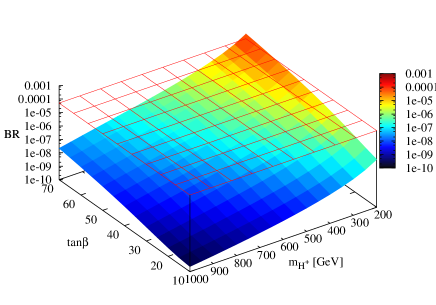
(a)

(b)

Figure 2: (a) 3D plot of $BR(t\to cH^{0})$ in the $m_{H^{+}}-\tan\beta$ plane in the T2HDM, and (b) the dominant diagram. We set $m_{h^{0}}=1000$ GeV and $m_{A^{0}}=1200$ GeV. The color scale represents the BR: the blue represents the lowest BR and red the highest.

The choice $m_{h^{0}}=1000$ GeV made in Fig. 2a suppresses the diagrams with $h^{0}$ in the loop and, thus, better explores the charged Higgs sector. As expected the BR rises with $\tan\beta$ and is highest when $m_{H^{+}}$ is lowest. The dominant Feynman diagram in this case is the one depicted in Fig. 2b with two $H^{+}$ and a $b$-quark in the loop. This diagram receives an enhancement from the 3-scalar vertex $H^{0}H^{+}H^{-}$, as noted above.

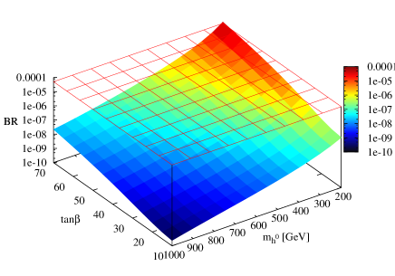
(a)

(b)

Figure 3: (a) 3D plot of $BR(t\to cH^{0})$ in the $m_{h^{0}}-\tan\beta$ plane in the T2HDM, and (b) the dominant diagram. We set $m_{H^{+}}=1000$ GeV and $m_{A^{0}}=1200$ GeV. See also caption to Fig. 2.

The choice $m_{H^{+}}=1000$ GeV made in Fig. 3a suppresses the diagrams with $H^{\pm}$ in the loop and, thus, is more sensitive to the neutral Higgs sector. In this case also, the BR rises with $\tan\beta$ and drops as $m_{h^{0}}$ is increased. The dominant diagram in this case is the one which has two $h^{0}$ scalars in the loop. This diagram receives an enhancement from the 3-scalar vertex $H^{0}h^{0}h^{0}$ when $m_{A^{0}}$ is large, as mentioned above.

The two limits $m_{h^{0}}=1000$ GeV and $m_{H^{+}}=1000$ GeV have similar consequences, yet the $BR\left(t\to cH^{0}\right)$ is higher when $m_{H^{+}}<m_{h^{0}}$ in which case the charged Higgs loop-exchange is the dominant source for the enhanced $BR\left(t\to cH^{0}\right)$. This is a distinctive property of the T2HDM, since, in this model, the charged Higgs coupling $H^{+}\bar{b}c$ is enhanced by $V_{tb}/V_{cb}$ compared to other 2HDM’s such as the type I and type II 2HDM.

In Fig. 4 we plot the $BR\left(t\to cH^{0}\right)$ in the $m_{A^{0}}-m_{h^{0}}$ plane, where all other parameters are given the central values of Eq. (20). We see that the BR is highest for a large $m_{A^{0}}$ and a small $m_{h^{0}}$ where the diagram with the two $h^{0}$ in the loop dominates. The dip in the middle of the surface is due to cancellations in the $H^{0}H^{+}H^{+}$ vertex.

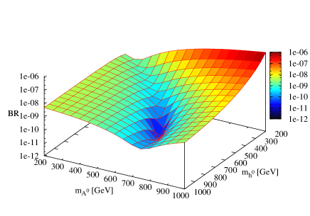
Figure 4: 3D plot of $BR(t\to cH^{0})$ in the $m_{A^{0}}-m_{h^{0}}$ plane in the T2HDM. We set $m_{H^{+}}=660$ GeV and $\tan\beta=28$.

To better illustrate the dependence of the $BR\left(t\to cH^{0}\right)$ on $\tan\beta$ and $m_{H^{+}}$ we give in Figs. 5 and 6 2D plots of the $BR\left(t\to cH^{0}\right)$ as a function of $\tan\beta$ and $m_{H^{+}}$, respectively, using the same parameter set as in Fig. 2.

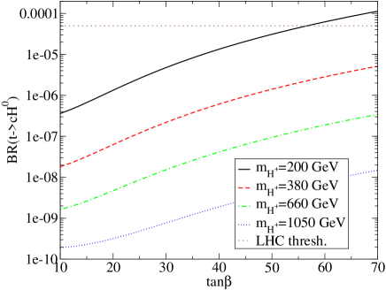
Figure 5: The $BR(t\to cH^{0})$ as a function of $\tan\beta$ at various $m_{H^{+}}$ in the T2HDM. We set $m_{h^{0}}=1000$ GeV and $m_{A^{0}}=1200$ GeV. “LHC thresh.” stands for the limit of the LHC sensitivity at 100 $fb^{-1}$.

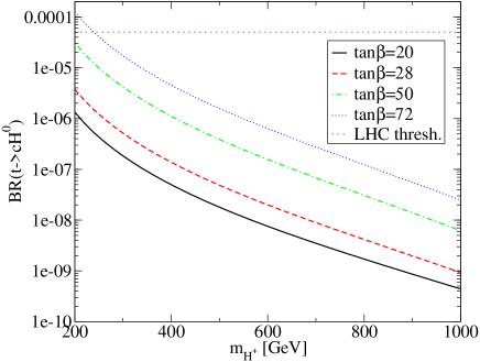
Figure 6: The $BR(t\to cH^{0})$ as a function of $m_{H^{+}}$ at various $\tan\beta$ in the T2HDM. We set $m_{h^{0}}=1000$ GeV and $m_{A^{0}}=1200$ GeV. “LHC thresh.” stands for the limit of the LHC sensitivity at 100 $fb^{-1}$.

Finally, in order to demonstrate the difference in the $BR\left(t\to cH^{0}\right)$ expected within the T2HDM, the 2HDM-II, and the SM , we list in table 2 the $BR\left(t\to cH^{0}\right)$ values within these 3 different models, for 4 different points in the relevant parameter space. Note that in the SM the 1-loop $BR\left(t\to cH^{0}\right)$ depends only on the SM’s Higgs mass which we also set to $m_{H^{0}}=91$ GeV. Also, recall that the type II 2HDM Yukawa potential is similar to that of the MSSM and that it has no tree-level FCNC.

$a^{b}$ parameters	SM	2HDM-II	T2HDM
$m_{h^{0}}=800$, $m_{A^{0}}=1000$, $\tan\beta=72$, $m_{H^{+}}=200$	$\vphantom{A^{A^{A}}}6.03\times 10^{-14}$	$4.25\times 10^{-5}$	$5.99\times 10^{-5}$
$m_{h^{0}}=800$, $m_{A^{0}}=1000$, $\tan\beta=72$, $m_{H^{+}}=380$	$\vphantom{A^{A^{A}}}6.03\times 10^{-14}$	$1.79\times 10^{-6}$	$2.57\times 10^{-6}$
$m_{h^{0}}=200$, $m_{A^{0}}=4000$, $\tan\beta=20$, $m_{H^{+}}=1050$	$\vphantom{A^{A^{A}}}6.03\times 10^{-14}$	$5.15\times 10^{-8}$	$9.39\times 10^{-5}$
$m_{h^{0}}=200$, $m_{A^{0}}=1000$, $\tan\beta=20$, $m_{H^{+}}=1050$	$\vphantom{A^{A^{A}}}6.03\times 10^{-14}$	$3.34\times 10^{-12}$	$3.14\times 10^{-7}$

Table 2: Comparison of the $BR(t\to cH^{0})$ within the T2HDM, the 2HDM-II, and the SM. Masses are in units of GeV.

The first two rows in table 2 illustrate the impact of the charged sector, by setting a high $m_{h^{0}}$ and a much smaller $m_{H^{+}}$ (note that the value $m_{H^{+}}=200$ GeV is outside the $1\sigma$ bounds). In this case, the $BR\left(t\to cH^{0}\right)$ in the T2HDM is not as enhanced as expected relative to the 2HDM-II, where it is a bit higher in the T2HDM. Recall that we expected the diagram with the $H^{+}$-$b$ quark in the loop to be particularly enhanced in the T2HDM due to the enhanced $H^{+}\bar{c}b$ interaction in this model. The amplitude of this diagram is (see App. C):

$$M_{7} =\frac{-i\bar{u}_{c}}{16\pi^{2}}g_{H^{+}H^{+}h}^{3h}\left[m_{b}C_{0}\left(A_{cb}^{H^{+}}B_{tb}^{H^{+}*}L+B_{cb}^{H^{+}}A_{tb}^{H^{+}*}R\right)\right.$$

$$-m_{c}C_{12}\left(B_{cb}^{H^{+}}B_{tb}^{H^{+}*}L+A_{cb}^{H^{+}}A_{tb}^{H^{+}*}R\right)$$

$$\left.+m_{t}\left(-C_{11}+C_{12}\right)\left(A_{cb}^{H^{+}}A_{tb}^{H^{+}*}L+B_{cb}^{H^{+}}B_{tb}^{H^{+}*}R\right)\right]u_{t},$$ (39)

where $C_{ij}$ are the Passarino-Veltman scalar functions. The term $\propto m_{b}A_{cb}^{H^{+}}B_{tb}^{H^{+}*}$ (multiplied by the left projection operator), which is sub-leading in the type II 2HDM, is enhanced in the T2HDM and dominates the other terms, being $\propto\xi^{*}m_{c}m_{b}^{2}\tan^{2}\beta V_{tb}V_{tb}^{*}$. On the other hand, in the 2HDM of type II it is the term $\propto m_{t}B_{cb}^{H^{+}}B_{tb}^{H^{+}*}\sim m_{t}m_{b}^{2}\tan^{2}\beta V_{cb}V_{tb}^{*}$ which dominates for a large $\tan\beta\gtrsim 10$. Therefore, we see that the different leading terms in the T2HDM and the type II 2HDM are roughly of the same order of magnitude since $m_{t}\cdot V_{cb}\sim m_{c}$, and therefore the enhancement in the T2HDM is not as significant as expected.

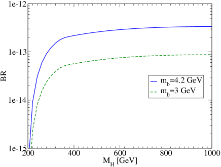
Figure 7: The SM value for the $BR(H^{0}\to\bar{t}c+\bar{c}t)$ as a function of the Higgs mass, for $\overline{m_{b}}(\overline{m_{b}})=4.2$ GeV and for $\overline{m_{b}}(\overline{m_{Z}})=3$ GeV PDG . The BR is not sensitive to $m_{c}$.

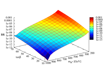
(a)

(b)

Figure 8: (a) 3D plot of $BR(H^{0}\to\bar{t}c+\bar{c}t)$ in the $m_{H^{+}}-\tan\beta$ plane in the T2HDM, and (b) the dominant diagram. We set $m_{h^{0}}=1000$ GeV and $m_{A^{0}}=1000$ GeV.

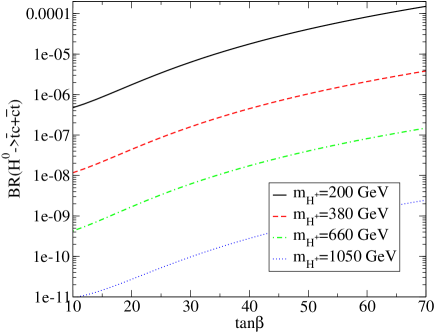
Figure 9: The $BR(H^{0}\to\bar{t}c+\bar{c}t)$ as a function of $\tan\beta$ at different $m_{H^{+}}$ in the T2HDM. We set $m_{h^{0}}=1000$ GeV and $m_{A^{0}}=1000$ GeV.

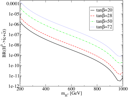
Figure 10: The $BR(H^{0}\to\bar{t}c+\bar{c}t)$ as a function of $m_{H^{+}}$ at different $\tan\beta$ in the T2HDM. We set $m_{h^{0}}=1000$ GeV and $m_{A^{0}}=1000$ GeV.

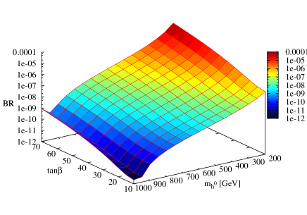
(a)

(b)

Figure 11: (a) 3D plot of $BR(H^{0}\to\bar{t}c+\bar{c}t)$ in the $m_{h^{0}}-\tan\beta$ plane in the T2HDM, and (b) the dominant diagram. We set $m_{H^{+}}=1000$ GeV and $m_{A^{0}}=1000$ GeV.

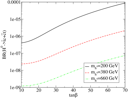
Figure 12: The $BR(H^{0}\to\bar{t}c+\bar{c}t)$ as a function of $\tan\beta$ at different $m_{h^{0}}$ in the T2HDM. We set $m_{H^{+}}=1000$ GeV and $m_{A^{0}}=1000$ GeV.

$a^{b}$ parameters	SM	2HDM-II	T2HDM
$m_{h^{0}}=800$, $m_{A^{0}}=1000$, $\tan\beta=72$, $m_{H^{+}}=200$	$\vphantom{A^{A^{A}}}1.23\times 10^{-13}$	$1.26\times 10^{-4}$	$1.70\times 10^{-4}$
$m_{h^{0}}=800$, $m_{A^{0}}=1000$, $\tan\beta=72$, $m_{H^{+}}=380$	$\vphantom{A^{A^{A}}}1.23\times 10^{-13}$	$3.09\times 10^{-6}$	$4.45\times 10^{-6}$
$m_{h^{0}}=200$, $m_{A^{0}}=4000$, $\tan\beta=20$, $m_{H^{+}}=1050$	$\vphantom{A^{A^{A}}}1.23\times 10^{-13}$	$8.69\times 10^{-8}$	$2.90\times 10^{-4}$
$m_{h^{0}}=200$, $m_{A^{0}}=1000$, $\tan\beta=20$, $m_{H^{+}}=1050$	$\vphantom{A^{A^{A}}}1.23\times 10^{-13}$	$8.99\times 10^{-12}$	$9.11\times 10^{-7}$

Table 3: Comparison of $BR(H^{0}\to\bar{t}c+\bar{c}t)$ between the T2HDM, the 2HDM-II, and the SM. Masses are in units of GeV. We set $m_{H^{0}}=300$, $\alpha=\beta$, and other parameters to their best-fit value of (20).

In the last two rows of table 2 we set a high $m_{H^{+}}\sim 1$ TeV, thus exploring the impact of an EW-scale neutral Higgs sector. Evidently, in this case the $BR\left(t\to cH^{0}\right)$ is much larger in the T2HDM than in the 2HDM of type II. This is in fact expected since the type II 2HDM does not have any tree-level FCNC.

VI.2 The 1-loop decay $H^{0}\to\bar{t}c$

In the results that follow, we assume that the Higgs decays that enter its total width (when kinematically allowed) are: $H^{0}\to\bar{q}q$, $H^{0}\to VV$, $H^{0}\to h_{i}h_{j}$ and $H^{0}\to V_{i}h_{j}$. The partial widths for these decay channels are given in App. D.

We first plot in Fig. 7 the SM value for the $BR\left(H^{0}\to\bar{t}c+\bar{c}t\right)$, as a function of the Higgs mass, for two b-quark masses: $\overline{m_{b}}(\overline{m_{b}})=4.2$ GeV and $\overline{m_{b}}(\overline{m_{Z}})=3$ GeV. Our results are in agreement with the results reported in h-tc SM arhrib .

Next we turn to our results in the T2HDM. In Fig. 8 we give a 3D plot of $BR\left(H^{0}\to\bar{t}c+\bar{c}t\right)$ in the $m_{H^{+}}-\tan\beta$ plane and in Figs. 9 and 10 we plot (2D) the BR as a function of $\tan\beta$ and $m_{H^{+}}$, respectively, with the same parameters as in Fig. 8. We again see the same tendency as in the case of $t\to cH^{0}$, i.e., the BR rises with $\tan\beta$ and decreases with $m_{H^{+}}$.

In Fig. 11 we give a 3D plot of the $BR\left(H^{0}\to\bar{t}c+\bar{c}t\right)$ in the $m_{h^{0}}-\tan\beta$ plane, and in Fig. 12 we plot (2D) the BR as a function of $\tan\beta$ with the same parameters as Fig. 11 for several values of $m_{h^{0}}$. We again see that the BR decreases with $m_{h^{0}}$ and increases with $\tan\beta$.

Finally, in table 3 we give the $BR\left(H^{0}\to\bar{t}c+\bar{c}t\right)$ in the three different models (SM, type II 2HDM and the T2HDM) for 4 points of the relevant parameter space. As can be seen, the behavior is similar to the reversed top decay $t\to cH^{0}$ process, albeit the $BR\left(H^{0}\to\bar{t}c+\bar{c}t\right)$ are typically higher.

VII Summary

We have studied the top and neutral Higgs FCNC rare decays $t\to ch$ and $h\to\bar{t}c$ ($h=h^{0}$ or $H^{0}$ are the two CP-even neutral Higgs) within the T2HDM. In this model the Higgs doublet with the heavier VEV ($v_{2}$) couples only to the top-quark, while the lighter Higgs doublet (i.e., with $v_{1}\ll v_{2}$) couples to all other quarks. In particular, the working assumption of the T2HDM is that $\tan\beta\equiv v_{2}/v_{1}\gg 1$, so that the top quark receives a much larger mass than all other quarks in a natural manner.

The Yukawa sector of the T2HDM exibits potentially enhanced FCNC in the up-quark sector and large flavor transitions mediated by the charged Higgs. These Yukawa interactions and the scalar self interactions of the model were explicitly (and independently) derived. For example, it was shown that the $H^{+}\bar{b}c$ Yukawa coupling, which (in this model) is enhanced by a factor of $V_{tb}/V_{cb}$ compared to the corresponding 2HDM type II coupling, enhances the 1-loop $t\to cH^{0}$ and $H^{0}\to\bar{t}c$ decays via diagrams involving $H^{+}$ and $b$-quarks inside the loop. Another potential enhancement of these 1-loop decays can come from the FCNC $h^{0}\bar{t}c$ Yukawa interaction, i.e., via diagrams containing $h^{0}$ and $t$-quarks.

Without loss of generality, we have considered the region in parameter space in which decays involving $h^{0}$ occur at tree-level while those involving $H^{0}$ are 1-loop mediated. We then explored the parameter space of the T2HDM for the resulting decays and found that the BR’s for the tree-level decays $t\to ch^{0}$ and $h^{0}\to\bar{t}c$ are typically of ${\cal O}(0.01)$, while the BR’s for the 1-loop decays $t\to cH^{0}$ and $H^{0}\to\bar{t}c$ can reach $10^{-5}-10^{-4}$ in a favorable scenario - a value higher than the LHC detection threshold for the top-decay and above their expected value within the SM and the type I and II 2HDM. Thus, even if $h^{0}$ decouples (i.e., too heavy), the 1-loop FCNC top-decay $t\to cH^{0}$ may still be accessible to the LHC.

Appendix A Feynman rules for two Higgs doublet models

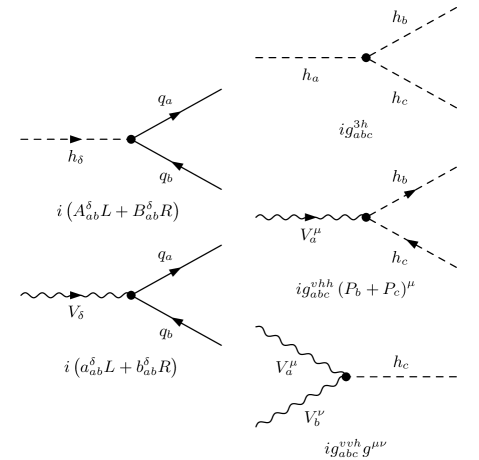
Figure 13: Feynman rules.

	$=ig_{abc}^{vhh}\left(P_{b}+P_{c}\right)^{\mu}$
$W^{+}H^{+}H^{0}$	$i\frac{g}{2}\sin\left(\beta-\alpha\right)\left(P_{H^{+}}+P_{H^{0}}\right)^{\mu}$
$W^{+}H^{+}h^{0}$	$-i\frac{g}{2}\cos\left(\beta-\alpha\right)\left(P_{H^{+}}+P_{h^{0}}\right)^{\mu}$
$W^{+}G^{+}H^{0}$	-$i\frac{g}{2}\cos\left(\beta-\alpha\right)\left(P_{G^{+}}+P_{H^{0}}\right)^{\mu}$
$W^{+}G^{+}h^{0}$	$-i\frac{g}{2}\sin\left(\beta-\alpha\right)\left(P_{G^{+}}+P_{h^{0}}\right)^{\mu}$
$Z^{0}A^{0}H^{0}$	$-\frac{g\sin\left(\beta-\alpha\right)}{2\cos\theta_{W}}\left(P_{A^{0}}+P_{H^{0}}\right)^{\mu}$
$Z^{0}A^{0}h^{0}$	$\frac{g\cos\left(\beta-\alpha\right)}{2\cos\theta_{W}}\left(P_{A^{0}}+P_{h^{0}}\right)^{\mu}$

Table 4: Feynman rules for vector-scalar-scalar interactions as in HHG . The second particle is outgoing.

$H^{+}H^{-}H^{0}$	$-\frac{g}{m_{W}}\left[\left(m_{H^{+}}^{2}-m_{A^{0}}^{2}+\frac{1}{2}m_{H^{0}}^{2}\right)\cos\left(\beta-\alpha\right)\right.$ $\left.\qquad\quad+\left(m_{A^{0}}^{2}-m_{H^{0}}^{2}\right)\cot 2\beta\sin\left(\beta-\alpha\right)\right]$
$H^{+}H^{-}h^{0}$	$-\frac{g}{m_{W}}\left[\left(m_{H^{+}}^{2}-m_{A^{0}}^{2}+\frac{1}{2}m_{h^{0}}^{2}\right)\sin\left(\beta-\alpha\right)\right.$ $\left.\qquad\quad+\left(m_{h^{0}}^{2}-m_{A^{0}}^{2}\right)\cot 2\beta\cos\left(\beta-\alpha\right)\right]$
$h^{0}h^{0}H^{0}$	$-\frac{g\cos\left(\beta-\alpha\right)}{2m_{W}\sin 2\beta}\left[\left(2m_{h^{0}}^{2}+m_{H^{0}}^{2}\right)\sin 2\alpha\right.$ $\left.\qquad\qquad\quad-m_{A^{0}}^{2}\left(3\sin 2\alpha-\sin 2\beta\right)\right]$
$h^{0}H^{0}H^{0}$	$-\frac{g\sin\left(\beta-\alpha\right)}{2m_{W}\sin 2\beta}\left[\left(2m_{H^{0}}^{2}+m_{h^{0}}^{2}\right)\sin 2\alpha\right.$ $\left.\qquad\qquad\quad-m_{A^{0}}^{2}\left(3\sin 2\alpha+\sin 2\beta\right)\right]$
$A^{0}A^{0}H^{0}$	$-\frac{g}{2m_{W}}\left[m_{H^{0}}^{2}\cos\left(\beta-\alpha\right)\right.$ $\left.\qquad\quad+2\left(m_{H^{0}}^{2}-m_{A^{0}}^{2}\right)\cot 2\beta\sin\left(\beta-\alpha\right)\right]$
$A^{0}A^{0}h^{0}$	$-\frac{g}{2m_{W}}\left[m_{h^{0}}^{2}\sin\left(\beta-\alpha\right)\right.$ $\left.\qquad\quad+2\left(m_{h^{0}}^{2}-m_{A^{0}}^{2}\right)\cot 2\beta\cos\left(\beta-\alpha\right)\right]$
$H^{+}G^{-}H^{0}$	$-i\frac{g}{2m_{W}}\left(m_{H^{+}}^{2}-m_{H^{0}}^{2}\right)\sin\left(\beta-\alpha\right)$
$H^{+}G^{-}h^{0}$	$i\frac{g}{2m_{W}}\left(m_{H^{+}}^{2}-m_{h^{0}}^{2}\right)\cos\left(\beta-\alpha\right)$
$G^{+}G^{-}H^{0}$	-$i\frac{g}{2m_{W}}m_{H^{0}}^{2}\cos\left(\beta-\alpha\right)$
$G^{+}G^{-}h^{0}$	$-i\frac{g}{2m_{W}}m_{h^{0}}^{2}\sin\left(\beta-\alpha\right)$

Table 5: Feynman rules for triple-scalar interactions bejar ; HHG .

	T2HDM	2HDM-II HHG
$H^{0}\bar{u}_{j}u_{i}$	$\frac{g}{2m_{W}}\left(-M_{u}\frac{\cos\alpha}{\cos\beta}+\Sigma\left(-\frac{\sin\alpha}{\sin\beta}+\frac{\cos\alpha}{\cos\beta}\right)\right)R+\left(h.c.\right)L$	$-\frac{gM_{u}}{2m_{W}}\frac{\sin\alpha}{\sin\beta}$
$h^{0}\bar{u}u$	$\frac{g}{2m_{W}}\left(M_{u}\frac{\sin\alpha}{\cos\beta}-\Sigma\left(\frac{\cos\alpha}{\sin\beta}+\frac{\sin\alpha}{\cos\beta}\right)\right)R+\left(h.c.\right)L$	$-\frac{gM_{u}}{2m_{W}}\frac{\cos\alpha}{\sin\beta}$
$A^{0}\bar{u}u$	$i\frac{g}{2m_{W}}\left(-M_{u}\tan\beta+\Sigma\left(\tan\beta+\cot\beta\right)\right)R+\left(h.c.\right)L$	$i\frac{gM_{u}}{2m_{W}}\cot\beta\left(R-L\right)$
$G^{0}\bar{u}u$	$i\frac{gM_{u}}{2m_{W}}\left(R-L\right)$	$i\frac{gM_{u}}{2m_{W}}\left(R-L\right)$
$H^{0}\bar{d}d$	$-\frac{gM_{d}}{2m_{W}}\frac{\cos\alpha}{\cos\beta}$	$-\frac{gM_{d}}{2m_{W}}\frac{\cos\alpha}{\cos\beta}$
$h^{0}\bar{d}d$	$\frac{gM_{d}}{2m_{W}}\frac{\sin\alpha}{\cos\beta}$	$\frac{gM_{d}}{2m_{W}}\frac{\sin\alpha}{\cos\beta}$
$A^{0}\bar{d}d$	$i\frac{gM_{d}}{2m_{W}}\tan\beta\left(R-L\right)$	$i\frac{gM_{d}}{2m_{W}}\tan\beta\left(R-L\right)$
$G^{0}\bar{d}d$	$-i\frac{gM_{d}}{2m_{W}}\left(R-L\right)$	$-i\frac{gM_{d}}{2m_{W}}\left(R-L\right)$
$H^{+}\bar{u}d$	$\frac{g}{\sqrt{2}m_{W}}\left[\tan\beta V_{CKM}M_{d}R+\right.$ $\left.+\left(-M_{u}\tan\beta+\Sigma\left(\tan\beta+\cot\beta\right)\right)V_{CKM}L\right]$	$\frac{g}{\sqrt{2}m_{W}}\left[\tan\beta V_{CKM}M_{d}R+\right.$ $\left.\qquad+\cot\beta M_{u}V_{CKM}L\right]$
$G^{+}\bar{u}d$	$\frac{g}{\sqrt{2}m_{W}}\left(M_{u}V_{CKM}L-V_{CKM}M_{d}R\right)$	$\frac{g}{\sqrt{2}m_{W}}\left(M_{u}V_{CKM}L-V_{CKM}M_{d}R\right)$

Table 6: Feynman rules for Yukawa interactions in the T2HDM and in the 2HDM-II.

$W^{+}W^{-}H^{0}$	$igm_{W}\cos\left(\beta-\alpha\right)g^{\mu\nu}$
$W^{+}W^{-}h^{0}$	$igm_{W}\sin\left(\beta-\alpha\right)g^{\mu\nu}$
$Z^{0}Z^{0}H^{0}$	$\frac{igm_{Z}}{\cos\theta_{W}}\cos\left(\beta-\alpha\right)g^{\mu\nu}$
$Z^{0}Z^{0}h^{0}$	$\frac{igm_{Z}}{\cos\theta_{W}}\sin\left(\beta-\alpha\right)g^{\mu\nu}$

Table 7: Feynman rules for vector-vector-scalar interactions HHG .

The relevant Feynman rules for the 2HDM’s that were used in this work are summarized in Fig. 13 and in Tables 6, 7, 4 and 5. The notation is given in Fig. 13 and the various couplings in the T2HDM and in the 2HDM of type II are collected in the Tables.

In particular, in Table 6 we list the Yukawa couplings, in Table 7 we give the vector-vector-scalar couplings, in Table 4 we give the vector-scalar-scalar couplings and the triple-scalar couplings, which are common to any 2HDM HHG , are given in Table 5. Note that the vertices $Z^{0}G^{0}H^{0}$ and $Z^{0}G^{0}h^{0}$ do not participate in the calculations since the corresponding Yukawa vertex $\bar{q}qG^{0}$ does not generate FCNC.

Appendix B 1-loop amplitudes

Here we give the 1-loop amplitudes corresponding to the 10 diagrams shown in Fig. 1. The calculation was done in the t’Hooft Feynman gauge and the following notation was used:

definitions:

$M_{n}$ – the amplitude corresponding to diagram $n$.
$h$ – the external neutral scalar.
$i$ – ($=t$) when used as index, the incoming fermion - the top.
$j$ – ($=c$) when used as index, the outgoing fermion - the charm.
$\alpha,\beta$ – when used as indices, internal bosons (vectors or scalars) in the loop.
$l,k,q$ – when used as indices, internal fermions.
$L,R$ – the Left,Right projection operators.
$\bar{u}_{j}$ – ($=\bar{u}(P_{j})$ ) the outgoing spinor of the charm.
$u_{i}$ – ($=u(P_{i})$ ) the incoming spinor of the top.
$B_{0},B_{1},C_{0},C_{ij}$ – the n-point integral functions, defined in App. C.
$A_{ab}^{\delta},B_{ab}^{\delta}$ – the left,right -handed parts of the fermion-fermion-scalar vertex.
$a_{ab}^{\delta},b_{ab}^{\delta}$ – the left,right -handed parts of the fermion-fermion-vector vertex, for both charged and neutral gauge bosons.
$g_{abc}^{3h,vhh,vvh}$ – the vertex of 3-scalars, vector-scalar-scalar, vector-vector-scalar, respectively.

$$M_{1} =\frac{i\bar{u}_{j}}{16\pi^{2}}\frac{-1}{m_{i}^{2}-m_{l}^{2}}\left[m_{l}m_{k}B_{0}\left(B_{lj}^{h*}A_{lk}^{\alpha}B_{ik}^{\alpha*}L+A_{lj}^{h*}B_{lk}^{\alpha}A_{ik}^{\alpha*}R\right)-m_{l}m_{i}B_{1}\left(B_{lj}^{h*}A_{lk}^{\alpha}A_{ik}^{\alpha*}L+A_{lj}^{h*}B_{lk}^{\alpha}B_{ik}^{\alpha*}R\right)\right.$$

$$\qquad\left.+m_{i}m_{k}B_{0}\left(B_{lj}^{h*}B_{lk}^{\alpha}A_{ik}^{\alpha*}L+A_{lj}^{h*}A_{lk}^{\alpha}B_{ik}^{\alpha*}R\right)-m_{i}^{2}B_{1}\left(B_{lj}^{h*}B_{lk}^{\alpha}B_{ik}^{\alpha*}L+A_{lj}^{h*}A_{lk}^{\alpha}A_{ik}^{\alpha*}R\right)\right]u_{i},$$ (40)

where $B=B\left(m_{k}^{2},m_{\alpha}^{2},m_{i}^{2}\right).$

$$M_{2} =\frac{i\bar{u}_{j}}{16\pi^{2}}\frac{-1}{m_{j}^{2}-m_{l}^{2}}\left[m_{l}m_{k}B_{0}\left(A_{jk}^{\alpha}B_{lk}^{\alpha*}B_{il}^{h*}L+B_{jk}^{\alpha}A_{lk}^{\alpha*}A_{il}^{h*}R\right)+m_{k}m_{j}B_{0}\left(B_{jk}^{\alpha}A_{lk}^{\alpha*}B_{il}^{h*}L+A_{jk}^{\alpha}B_{lk}^{\alpha*}A_{il}^{h*}R\right)\right.$$

$$\qquad\left.-m_{j}m_{l}B_{1}\left(B_{jk}^{\alpha}B_{lk}^{\alpha*}B_{il}^{h*}L+A_{jk}^{\alpha}A_{lk}^{\alpha*}A_{il}^{h*}R\right)-m_{j}^{2}B_{1}\left(A_{jk}^{\alpha}A_{lk}^{\alpha*}B_{il}^{h*}L+B_{jk}^{\alpha}B_{lk}^{\alpha*}A_{il}^{h*}R\right)\right]u_{i},$$ (41)

where $B=B\left(m_{k}^{2},m_{\alpha}^{2},m_{j}^{2}\right).$

$$M_{3} =\frac{i\bar{u}_{j}}{16\pi^{2}}\frac{1}{m_{i}^{2}-m_{l}^{2}}\left[4m_{l}m_{k}B_{0}\left(B_{lj}^{h*}b_{lk}^{\alpha}a_{ik}^{\alpha*}L+A_{lj}^{h*}a_{lk}^{\alpha}b_{ik}^{\alpha*}R\right)+2m_{l}m_{i}B_{1}\left(B_{lj}^{h*}b_{lk}^{\alpha}b_{ik}^{\alpha*}L+A_{lj}^{h*}a_{lk}^{\alpha}a_{ik}^{\alpha*}R\right)\right.$$

$$\qquad\left.+4m_{i}m_{k}B_{0}\left(B_{lj}^{h*}a_{lk}^{\alpha}b_{ik}^{\alpha*}L+A_{lj}^{h*}b_{lk}^{\alpha}a_{ik}^{\alpha*}R\right)+2m_{i}^{2}B_{1}\left(B_{lj}^{h*}a_{lk}^{\alpha}a_{ik}^{\alpha*}L+A_{lj}^{h*}b_{lk}^{\alpha}b_{ik}^{\alpha*}R\right)\right]u_{i},$$ (42)

where $B=B\left(m_{k}^{2},m_{\alpha}^{2},m_{i}^{2}\right).$

$$M_{4} =\frac{i\bar{u}_{j}}{16\pi^{2}}\frac{1}{m_{j}^{2}-m_{l}^{2}}\left[4m_{l}m_{k}B_{0}\left(b_{jk}^{\alpha}a_{lk}^{\alpha*}B_{il}^{h*}L+a_{jk}^{\alpha}b_{lk}^{\alpha*}A_{il}^{h*}R\right)+4m_{k}m_{j}B_{0}\left(a_{jk}^{\alpha}b_{lk}^{\alpha*}B_{il}^{h*}L+b_{jk}^{\alpha}a_{lk}^{\alpha*}A_{il}^{h*}R\right)\right.$$

$$\qquad\left.+2m_{j}m_{l}B_{1}\left(a_{jk}^{\alpha}a_{lk}^{\alpha*}B_{il}^{h*}L+b_{jk}^{\alpha}b_{lk}^{\alpha*}A_{il}^{h*}R\right)+2m_{j}^{2}B_{1}\left(b_{jk}^{\alpha}b_{lk}^{\alpha*}B_{il}^{h*}L+a_{jk}^{\alpha}a_{lk}^{\alpha*}A_{il}^{h*}R\right)\right]u_{i},$$ (43)

where $B=B\left(m_{k}^{2},m_{\alpha}^{2},m_{j}^{2}\right).$

$$M_{5} =\frac{-i\bar{u}_{j}}{16\pi^{2}}\left(A_{jq}^{\alpha}L+B_{jq}^{\alpha}R\right)\left\{\left[\tilde{C}_{0}+m_{i}^{2}C_{11}+\left(m_{h}^{2}-m_{i}^{2}\right)C_{12}\right]\left(A_{jq}^{\alpha}A_{kq}^{h*}B_{ik}^{\alpha*}L+B_{jq}^{\alpha}B_{kq}^{h*}A_{ik}^{\alpha*}R\right)\right.$$

$$-m_{q}m_{i}C_{11}\left(A_{jq}^{\alpha}B_{kq}^{h*}A_{ik}^{\alpha*}L+B_{jq}^{\alpha}A_{kq}^{h*}B_{ik}^{\alpha*}R\right)+m_{q}m_{j}C_{12}\left(B_{jq}^{\alpha}A_{kq}^{h*}B_{ik}^{\alpha*}L+A_{jq}^{\alpha}B_{kq}^{h*}A_{ik}^{\alpha*}R\right)$$

$$+m_{i}m_{j}\left(C_{12}-C_{11}\right)\left(B_{jq}^{\alpha}B_{kq}^{h*}A_{ik}^{\alpha*}L+A_{jq}^{\alpha}A_{kq}^{h*}B_{ik}^{\alpha*}R\right)+m_{q}m_{k}C_{0}\left(A_{jq}^{\alpha}B_{kq}^{h*}B_{ik}^{\alpha*}L+B_{jq}^{\alpha}A_{kq}^{h*}A_{ik}^{\alpha*}R\right)$$

$$\left.-m_{i}m_{k}\left(C_{11}+C_{0}\right)\left(A_{jq}^{\alpha}A_{kq}^{h*}A_{ik}^{\alpha*}L+B_{jq}^{\alpha}B_{kq}^{h*}B_{ik}^{\alpha*}R\right)+m_{j}m_{k}\left(C_{12}+C_{0}\right)\left(B_{jq}^{\alpha}B_{kq}^{h*}B_{ik}^{\alpha*}L+A_{jq}^{\alpha}A_{kq}^{h*}A_{ik}^{\alpha*}R\right)\right\}u_{i},$$ (44)

where $C=C\left(m_{k}^{2},m_{\alpha}^{2},m_{q}^{2},m_{i}^{2},m_{j}^{2},m_{h}^{2}\right).$

$$M_{6} =\frac{i\bar{u}_{j}}{16\pi^{2}}\left\{\left[4\tilde{C}_{0}+2\left(m_{i}^{2}-m_{j}^{2}+m_{h}^{2}\right)C_{11}+2\left(-m_{i}^{2}+m_{j}^{2}+m_{h}^{2}\right)C_{12}\right]\left(b_{jq}^{\alpha}B_{kq}^{h*}a_{ik}^{\alpha*}L+a_{jq}^{\alpha}A_{kq}^{h*}b_{ik}^{\alpha*}R\right)\right.$$

$$+2m_{q}m_{i}C_{11}\left(b_{jq}^{\alpha}A_{kq}^{h*}b_{ik}^{\alpha*}L+a_{jq}^{\alpha}B_{kq}^{h*}a_{ik}^{\alpha*}R\right)-2m_{q}m_{j}C_{12}\left(a_{jq}^{\alpha}B_{kq}^{h*}a_{ik}^{\alpha*}L+b_{jq}^{\alpha}A_{kq}^{h*}b_{ik}^{\alpha*}R\right)$$

$$+4m_{q}m_{k}C_{0}\left(b_{jq}^{\alpha}A_{kq}^{h*}a_{ik}^{\alpha*}L+a_{jq}^{\alpha}B_{kq}^{h*}b_{ik}^{\alpha*}R\right)+2m_{i}m_{k}\left(C_{11}+C_{0}\right)\left(b_{jq}^{\alpha}B_{kq}^{h*}b_{ik}^{\alpha*}L+a_{jq}^{\alpha}A_{kq}^{h*}a_{ik}^{\alpha*}R\right)$$

$$\left.-2m_{j}m_{k}\left(C_{12}+C_{0}\right)\left(a_{jq}^{\alpha}A_{kq}^{h*}a_{ik}^{\alpha*}L+b_{jq}^{\alpha}B_{kq}^{h*}b_{ik}^{\alpha*}R\right)\right\}u_{i},$$ (45)

where $C=C\left(m_{k}^{2},m_{\alpha}^{2},m_{q}^{2},m_{i}^{2},m_{j}^{2},m_{h}^{2}\right).$

$$M_{7} =\frac{-i\bar{u}_{j}}{16\pi^{2}}g_{\alpha\beta h}^{3h}\left[m_{k}C_{0}\left(A_{jk}^{\beta}B_{ik}^{\alpha*}L+B_{jk}^{\beta}A_{ik}^{\alpha*}R\right)-m_{j}C_{12}\left(B_{jk}^{\beta}B_{ik}^{\alpha*}L+A_{jk}^{\beta}A_{ik}^{\alpha*}R\right)\right.$$

$$\left.\qquad\qquad+m_{i}\left(-C_{11}+C_{12}\right)\left(A_{jk}^{\beta}A_{ik}^{\alpha*}L+B_{jk}^{\beta}B_{ik}^{\alpha*}R\right)\right]u_{i},$$ (46)

where $C=C\left(m_{k}^{2},m_{\alpha}^{2},m_{\beta}^{2},m_{i}^{2},m_{h}^{2},m_{j}^{2}\right).$

$$M_{8} =\frac{-i\bar{u}_{j}}{16\pi^{2}}g_{\alpha\beta h}^{vvh}\left[4m_{k}C_{0}\left(b_{jk}^{\beta}a_{ik}^{\alpha*}L+a_{jk}^{\beta}b_{ik}^{\alpha*}R\right)+2m_{i}\left(C_{11}-C_{12}\right)\left(b_{jk}^{\beta}b_{ik}^{\alpha*}L+a_{jk}^{\beta}a_{ik}^{\alpha*}R\right)\right.$$

$$\left.\qquad\qquad+2m_{j}C_{12}\left(a_{jk}^{\beta}a_{ik}^{\alpha*}L+b_{jk}^{\beta}b_{ik}^{\alpha*}R\right)\right]u_{i},$$ (47)

where $C=C\left(m_{k}^{2},m_{\alpha}^{2},m_{\beta}^{2},m_{i}^{2},m_{h}^{2},m_{j}^{2}\right).$

$$M_{9} =\frac{i\bar{u}_{j}}{16\pi^{2}}g_{\beta\alpha h}^{vhh}\left[\left(\tilde{C}_{0}+2m_{i}^{2}C_{11}+m_{j}^{2}C_{12}-2m_{h}^{2}C_{12}\right)\left(b_{jk}^{\beta}B_{ik}^{\alpha*}L+a_{jk}^{\beta}A_{ik}^{\alpha*}R\right)\right.$$

$$\qquad-m_{i}m_{j}\left(C_{12}+C_{11}\right)\left(a_{jk}^{\beta}A_{ik}^{\alpha*}L+b_{jk}^{\beta}B_{ik}^{\alpha*}R\right)+m_{j}m_{k}\left(C_{0}-C_{12}\right)\left(a_{jk}^{\beta}B_{ik}^{\alpha*}L+b_{jk}^{\beta}A_{ik}^{\alpha*}R\right)$$

$$\left.\qquad+m_{i}m_{k}\left(C_{12}-C_{11}-2C_{0}\right)\left(b_{jk}^{\beta}A_{ik}^{\alpha*}L+a_{jk}^{\beta}B_{ik}^{\alpha*}R\right)\right]u_{i},$$ (48)

where $C=C\left(m_{k}^{2},m_{\alpha}^{2},m_{\beta}^{2},m_{i}^{2},m_{h}^{2},m_{j}^{2}\right).$

$$M_{10} =\frac{i\bar{u}_{j}}{16\pi^{2}}g_{\alpha\beta h}^{vhh}\left[\left(-\tilde{C}_{0}+m_{i}^{2}\left(C_{12}-C_{11}\right)-2m_{j}^{2}C_{11}-2m_{h}^{2}\left(C_{12}-C_{11}\right)\right)\left(A_{jk}^{\beta}a_{ik}^{\alpha*}L+B_{jk}^{\beta}b_{ik}^{\alpha*}R\right)\right.$$

$$\qquad+m_{i}m_{j}\left(2C_{11}-C_{12}\right)\left(B_{jk}^{\beta}b_{ik}^{\alpha*}L+A_{jk}^{\beta}a_{ik}^{\alpha*}R\right)+m_{j}m_{k}\left(C_{12}+2C_{0}\right)\left(B_{jk}^{\beta}a_{ik}^{\alpha*}L+A_{jk}^{\beta}b_{ik}^{\alpha*}R\right)$$

$$\left.\qquad+m_{i}m_{k}\left(C_{11}-C_{12}-C_{0}\right)\left(A_{jk}^{\beta}b_{ik}^{\alpha*}L+B_{jk}^{\beta}a_{ik}^{\alpha*}R\right)\right]u_{i},$$ (49)

where $C=C\left(m_{k}^{2},m_{\alpha}^{2},m_{\beta}^{2},m_{i}^{2},m_{h}^{2},m_{j}^{2}\right).$

Appendix C 1-loop integrals

The 1-loop scalar, vector and tensor integrals are defined as:

$$B_{0};B_{\mu}\left(m_{1}^{2},m_{2}^{2},p^{2}\right) =\int\frac{d^{4}k}{i\pi^{2}}\frac{1;k_{\mu}}{\left[k^{2}-m_{1}^{2}\right]\left[\left(k+p\right)^{2}-m_{2}^{2}\right]},$$ (50)

$$C_{0};C_{\mu};C_{\mu\nu};\tilde{C}_{0}\left(m_{1}^{2},m_{2}^{2},m_{3}^{2},p_{1}^{2},p_{2}^{2},p_{3}^{2}\right)=$$

$$\int\frac{d^{4}k}{i\pi^{2}}\frac{1;k_{\mu};k_{\mu\nu};k^{2}}{\left[k^{2}-m_{1}^{2}\right]\left[\left(k+p_{1}\right)^{2}-m_{2}^{2}\right]\left[\left(k+p_{1}+p_{2}\right)^{2}-m_{3}^{2}\right]},$$ (51)

where $\sum_{i}p_{i}=0$ and the reduction to the 1-loop scalar functions is:

$${\rm B}_{\mu} =p_{\mu}{\rm B}_{1},$$

$${\rm C}_{\mu} =p_{1\mu}{\rm C}_{11}+p_{2\mu}{\rm C}_{12},$$

$${\rm C}_{\mu\nu} =p_{1\mu}p_{1\nu}{\rm C}_{21}+p_{2\mu}p_{2\nu}{\rm C}_{22}+\{p_{1}p_{2}\}_{\mu\nu}{\rm C}_{23}+g_{\mu\nu}{\rm C}_{24},$$ (52)

with $\{ab\}_{\mu\nu}\equiv a_{\mu}b_{\nu}+a_{\nu}b_{\mu}$.

Appendix D The Higgs width

The total Higgs width, $\Gamma^{tot}$, is derived from:

$$\Gamma^{tot}= \Gamma(h\to\bar{q}q)+\Gamma(h\to VV)$$

$$+\Gamma(h\to H_{i}H_{j})+\Gamma(h\to VH),$$ (53)

when kinematically allowed (i.e., the decay products are assumed to be on-shell). All the above partial widths were calculated at tree-level. The relevant couplings follow the definition in Fig. 13.

The decay width for $h\to\bar{q}q$ is HHG :

$$\Gamma\left(h\to\bar{q}q\right) =\frac{N_{c}A_{hqq}^{2}}{8\pi}m_{h}\left(1-\frac{4m_{q}^{2}}{m_{h}^{2}}\right)^{\frac{3}{2}}~{},$$ (54)

where $A_{hqq}=-\frac{gm_{q}}{2m_{W}}\frac{\cos\alpha}{\cos\beta}$; $\frac{gm_{q}}{2m_{W}}\frac{\sin\alpha}{\cos\beta}$ for $h=H^{0};~{}h^{0}$, respectively, and $N_{c}=3$. For example, the width for the decay $h^{0}\to\bar{b}b$ in the T2HDM with $\alpha=\beta$ is:

$$\Gamma\left(h^{0}\to\bar{b}b\right) =\frac{3g^{2}m_{b}^{2}}{32\pi m_{W}^{2}}m_{h^{0}}\tan^{2}\beta\left(1-\frac{4m_{b}^{2}}{m_{h^{0}}^{2}}\right)^{\frac{3}{2}}~{}.$$ (55)

The decay width for $h\to W^{+}W^{-}$ is HHG :

$$\Gamma\left(h\to W^{+}W^{-}\right) =\frac{g_{hWW}^{2}m_{h}^{3}}{64\pi m_{W}^{4}}\left(1-x\right)^{\frac{1}{2}}\left(1-x+\frac{3}{4}x^{2}\right)~{},$$ (56)

where $g_{hWW}=gm_{W}\cos\left(\beta-\alpha\right)$; $gm_{W}\sin\left(\beta-\alpha\right)$ for $h=H^{0};~{}h^{0}$, respectively, and $x=\frac{4m_{W}^{2}}{m_{h}^{2}}$.

The decay width for $h\to Z^{0}Z^{0}$ is HHG :

$$\Gamma\left(h\to Z^{0}Z^{0}\right) =\frac{g_{hZZ}^{2}m_{h}^{3}\cos^{4}\theta_{W}}{32\pi m_{W}^{4}}\left(1-x\right)^{\frac{1}{2}}\left(1-x+\frac{3}{4}x^{2}\right),$$ (57)

where $g_{hZZ}=\frac{gm_{Z}}{\cos\theta_{W}}\cos\left(\beta-\alpha\right)$; $\frac{gm_{Z}}{\cos\theta_{W}}\sin\left(\beta-\alpha\right)$ for $h=H^{0};~{}h^{0}$, respectively, and $x=\frac{4m_{Z}^{2}}{m_{h}^{2}}$. Note that by choosing $\alpha=\beta$ one sets the couplings $W^{+}W^{-}h^{0}$ and $Z^{0}Z^{0}h^{0}$ to zero in which case $\Gamma(h^{0}\to W^{+}W^{-}),~{}\Gamma(h^{0}\to Z^{0}Z^{0})=0$ while $\Gamma(H^{0}\to W^{+}W^{-})$ and $\Gamma(h^{0}\to Z^{0}Z^{0})$ are maximal.

The decay width for $h\to H_{i}H_{j}$ (where $H_{i},~{}H_{j}\neq h$) is:

$$\Gamma\left(h\to H_{i}H_{j}\right) =\frac{g_{hH_{i}H_{j}}^{2}}{16\pi m_{h}}\lambda^{\frac{1}{2}}\left(1,\frac{m_{H_{i}}^{2}}{m_{h}^{2}},\frac{m_{H_{j}}^{2}}{m_{h}^{2}}\right)~{},$$ (58)

where $g_{hH_{i}H_{j}}$ are the triple scalar couplings, and we recall that: $\lambda\left(x,y,z\right)=x^{2}+y^{2}+z^{2}-2xy-2xz-2yz$.

The decay width for $h\to VH$ (where $VH=W^{+}H^{-}$ or $VH=Z^{0}H_{i}^{0}$ and $H_{i}^{0}\neq h$) is:

$$\Gamma\left(h\to VH\right) =\frac{g_{VHh}^{2}m_{V}^{2}}{16\pi m_{h}}\lambda^{\frac{1}{2}}\left(1,\frac{m_{V}^{2}}{m_{h}^{2}},\frac{m_{H}^{2}}{m_{h}^{2}}\right)\lambda\left(1,\frac{m_{h}^{2}}{m_{V}^{2}},\frac{m_{H}^{2}}{m_{V}^{2}}\right)~{},$$ (59)

where $g_{hVH}$ are the vector-scalar-scalar couplings.

In order to demonstrate the role of radiative corrections to the leading order tree-level total width, we plot in Fig. 14 the total SM Higgs width at the tree-level (i.e., as calculated in this work) compared to the width calculated including higher-order corrections djouadi I . As can be seen, the discrepancy between the lowest order and the higher order calculations is significant only below the WW threshold (at about 160 GeV). In this mass range the $b\bar{b}$ decay channel dominates for which radiative corrections can have an appreciable impact. This mass range is, however, below the $h\to\bar{t}c$ threshold and therefore irrelevant to the present work, and so the use of the lowest order widths is justified.

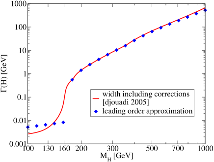
Figure 14: The total width of the SM Higgs: leading order approximation compared to the corrected (1-loop) width of djouadi I .

References

- (1) A. Das, C. Kao, “A two Higgs doublet model for the top quark”, Phys. Lett. B372, 106 (1996), arXiv:hep-ph/9511329.
- (2) S. Bejar, “Flavor changing neutral decay effects in models with two Higgs boson doublets: Applications to LHC Physics”, PhD thesis (2006), arXiv:hep-ph/0606138; S. Bejar, J. Guasch, J. Sola, “Loop Induced Flavor Changing Neutral Decays of the Top Quark in a General Two-Higgs-Doublet Model”, Nucl. Phys. B600, 21 (2001), arXiv:hep-ph/0011091.
- (3) J.A. Aguilar-Saavedra, ”Top flavor-changing neutral interactions: Theoretical expectations and experimental detection”, Acta Phys. Polon. B35, 2695 (2004), arXiv:hep-ph/0409342; J.A. Aguilar-Saavedra, G.C. Branco, “Probing top flavor changing neutral scalar couplings at the CERN LHC”, Phys. Lett. B495, 347 (2000), arXiv:hep-ph/0004190.
- (4) B. Grzadkowski, J.F. Gunion, P. Krawczyk, “Neutral Current Flavor Changing Decays for the Z Boson and the Top Quark in Two Higgs Doublet Models”, Phys. Lett. B268, 106-11 (1991), UCD-90-34, Dec 1990; J.L. Diaz-Cruz, R. Martinez,M.A. Perez and A. Rosado, “Flavor Changing Radiative Decay of the Top”, Phys. Rev. D41, 891 (1900); G. Eilam, J.L. Hewett, A. Soni, “Rare decays of the top quark in the standard and two Higgs doublet models”, Phys. Rev. D44, 1473 (1991), see also: Erratum, Phys. Rev. D59:039901 (1999); B. Mele, S. Petrarca, A. Soddu, ”A New evaluation of the decay width in the standard model”, Phys. Lett. B435, 401 (1998), arXiv:hep-ph/9805498.
- (5) A. Arhrib, “Higgs bosons decay into bottom-strange in two Higgs Doublets Models”, Phys. Lett. B612, 263 (2005), arXiv:hep-ph/0409218.
- (6) J. F. Gunion, H. E. Haber, G. Kane, S. Dawson, “The Higgs Hunter’s Guide”, Addison-Wesley (1990); see also: Errata, SCIPP-92-58 (1992), arXiv:hep-ph/9302272.
- (7) H. Georgi, “A model of soft CP violation”, Hadronic J. 1, 155 (1978).
- (8) D. Atwood, S. Bar-Shalom, G. Eilam, A. Soni, ”Flavor changing Z-decays from scalar interactions at a Giga-Z Linear Collider”, Phys. Rev. D66:093005 (2002), arXiv:hep-ph/0203200.
- (9) G.-H. Wu, A. Soni, “Novel CP-violating effects in B decays from a charged Higgs boson in a two-Higgs-doublet model for the top quark”. Phys. Rev. D62:056005 (2000), arXiv:hep-ph/9911419.
- (10) D. Atwood, L. Reina, A. Soni, “Phenomenology of two Higgs doublet models with flavor changing neutral currents”, Phys. Rev. D55, 3156 (1997), arXiv:hep-ph/9609279.
- (11) D. Atwood, S. Bar-Shalom, G. Eilam, A. Soni, “Three heavy jet events at hadron colliders as a sensitive probe of the Higgs sector”, Phys. Rev. D69:033006 (2004), arXiv:hep-ph/0309016.
- (12) I. Baum, “Top quark rare decays in a two Higgs doublet model for the top”, MSc Thesis (2007), arXiv:hep-ph/0711.1311.
- (13) E. Lunghi, A. Soni, “Footprints of the Beyond in flavor physics: Possible role of the Top Two Higgs Doublet Model”, J. of High Energy Physics 0709:053 (2007), arXiv:hep-ph/0707.0212.
- (14) A. Arhrib, “Top and Higgs Flavor Changing Neutral Couplings in two Higgs Doublets Model”, Phys. Rev. D72:075016 (2005), arXiv:hep-ph/0510107.
- (15) W.-M. Yao et al. (Particle Data Group), J. Phys. G33, 1 (2006) and 2007 partial update for the 2008 edition (URL: http://pdg.lbl.gov).
- (16) M. E. Peskin, D. V. Schroeder, ”An introduction to quantum field theory”, Perseus Books (1995).
- (17) G. J. van Oldenborgh, “FF: A Package to evaluate one loop Feynman diagrams”, NIKHEF-H-90-15 (1990); Comput. Phys. Commun. 66, 1 (1991); download: http://www.xs4all.nl/~gjvo/FF.html.
- (18) A. Djouadi, “The Anatomy of Electro-Weak Symmetry Breaking, II: The Higgs bosons in the Minimal Supersymmetric Model”, LPT-ORSAY-05-18 (2005), arXiv: hep-ph/0503173.
- (19) C.R. Das, M.K. Parida, “New formulae and predictions for running fermion masses at higher scales in SM, 2 HDM, and MSSM”, Eur. Phys. J. C20, 121 (2001), arXiv:hep-ph/0010004.
- (20) A. Djouadi, “The Anatomy of Electro-Weak Symmetry Breaking, I: The Higgs boson in the Standard Model”, LPT-ORSAY-05-18 (2005), arXiv:hep-ph/0503172.