Three-dimensional radiative transfer models of clumpy tori in Seyfert galaxies

Abstract

Context. Tori of Active Galactic Nuclei (AGN) are made up of a mixture of hot and cold gas, as well as dust. In order to protect the dust grains from destruction by the surrounding hot gas as well as by the energetic (UV/optical) radiation from the accretion disk, the dust is often assumed to be distributed in clouds.

Aims. A new three-dimensional model of AGN dust tori is extensively investigated. The torus is modelled as a wedge-shaped disk within which dusty clouds are randomly distributed throughout the volume, by taking the dust density distribution of the corresponding continuous model into account. We especially concentrate on the differences between clumpy and continuous models in terms of the temperature distributions, the surface brightness distributions and interferometric visibilities, as well as spectral energy distributions.

Methods. Radiative transfer calculations with the help of the three-dimensional Monte Carlo radiative transfer code MC3D are used in order to simulate spectral energy distributions as well as surface brightness distributions at various wavelengths. In a second step, interferometric visibilities for various inclination as well as position angles and baselines are calculated, which can be used to directly compare our models to interferometric observations with the MIDI instrument.

Results. We find that the radial temperature distributions of clumpy models possess significantly enhanced scatter compared to the continuous cases. Even at large distances, clouds can be heated directly by the central accretion disk. The existence of the silicate 10$\,\muup$m-feature in absorption or in emission depends sensitively on the distribution, the size and optical depth of clouds in the innermost part of the dust distribution. With this explanation, failure and success of previous modelling efforts of clumpy tori can be understood. The main reason for this outcome are shadowing effects of clouds within the central region. We underline this result with the help of several parameter variations. After adapting the parameters of our clumpy standard model to the circumstances of the Seyfert 2 Circinus galaxy, it can qualitatively explain recent mid-infrared interferometric observations performed with MIDI, as well as high resolution spectral data.

1 Introduction and motivation

According to today’s knowledge, Active Galactic Nuclei (AGN) are powered by accretion onto a supermassive black hole ($10^{6}-10^{10}\,M_{\odot}$, e.g. Shankar et al. 2004) residing in their centres. Thereby, gravitational energy is converted into heat by viscous processes within the surrounding accretion disk, which extends from the marginally stable orbit up to several thousands of Schwarzschild radii. The emitted UV/optical light illuminates the attached, toroidally shaped dust reservoir. The concept of this obscuring torus was introduced in order to unify mainly two classes of observed spectral energy distributions (SEDs): one shows a peak in the UV-region with overlayed broad and narrow optical emission lines, the other class shows only narrow optical emission lines. This can be interpreted as an inclination angle dependence. For viewing angles within the dust-free cone of the torus (type 1 sources), direct signatures of the accretion disk (a peak in the UV-range) and the region close to the centre within the funnel of the torus show up. This is where gas moves fast and, therefore, produces broad emission lines (the region is hence called the Broad Line Region (BLR) of the nucleus). For edge-on lines of sight (type 2 sources), the direct view onto the centre is blocked and optical emission lines can only be detected from gas beyond the torus funnel. Being further away from the centre, it moves slower and hence produces narrow emission lines only. This is the so-called Unified Scheme of Active Galactic Nuclei (Antonucci 1993; Urry & Padovani 1995). First evidence for this scenario came from spectropolarimetric observations of type 2 sources (Miller & Antonucci 1983), clearly displaying type 1 signatures in the polarised light, which is scattered by electrons and tenuous dust within the funnel above the torus. The opening angle of the torus can be estimated with the help of statistics of the different types of Seyfert galaxies. Maiolino & Rieke (1995) find a ratio between Sy 2 to Sy 1 galaxies of 4:1 in their sample, which results in an opening angle of the light cones of $74\degr$, in concordance with many observations of ionisation cones of individual galaxies. Direct support for the idea of geometrically thick tori comes from recent interferometric observations in the mid-infrared (e.g. Jaffe et al. 2004; Tristram et al. 2007).

These tori are made up of at least three components: (i) hot ionised gas, (ii) warm molecular gas and (iii) dust. Krolik & Begelman (1988) proposed that the dusty part has to be organised in a clumpy structure in order to prevent the grains from being destroyed by the hot surrounding gas (with temperatures of the order of $10^{6}\leavevmode\nobreak\$K) in which the clouds are supposed to be embedded. Another hint for the clumpy nature of the obscuring material – in this case mainly for the distribution of neutral gas – comes from X-ray measurements of the absorbing column density. Risaliti et al. (2002) claim that the observed variability of these measurements on timescales from months to several years can be explained by a clumpy structure of the torus. Combining X-ray absorbing column densities with spectral information further strengthens the claim for a clumpy distribution of the dust (Shi et al. 2006).

Earlier work on torus simulations concentrated mostly on smooth dust distributions (e.g. Pier & Krolik 1992a; Granato & Danese 1994; van Bemmel & Dullemond 2003; Schartmann et al. 2005). This was mainly caused by the lack of appropriate (3D) radiative transfer codes and computational power. Nevertheless, such models are good approximations for the case that the clumps that build up the torus are small compared to the total torus size, as is also shown in a parameter study described in Sect. 4.2. These continuous models are able to describe the gross observable features of these objects (see Schartmann et al. 2005, e. g.). However, problems arose from too strong emission features of silicate dust compared to the observations, when looking directly onto the inner rims of the model structures (face-on views). They had never been observed before that time, although almost all models showed them for the face-on view. Therefore, much theoretical effort was undertaken in order to find models showing no silicate feature at all in the face-on case, while retaining the silicate absorption feature in the edge-on case. Manske et al. (1998) for example succeeded in avoiding silicate emission features with a flared dust disk of high optical depth in combination with an anisotropic radiation characteristic of the central illuminating source. A very promising idea was to solve the problem naturally by splitting the dust distribution into single clouds. This was first attempted by Nenkova et al. (2002). A one-dimensional code for the simulation of radiative transfer through single clumps was used and, in a second step, the torus and its emitted SED was assembled by adding many clouds of different aspect angles with the help of a statistical method. With this approach, they could show that a clumpy dust distribution of this kind can significantly smear out the prominent silicate emission feature of the SEDs of type 1 objects at $10\,\muup$m for a large range of parameter values. No more fine-tuning was needed, as in the previously proposed solutions with the help of special continuous models. Subsequently, real two-dimensional radiative transfer calculations were undertaken by Dullemond & van Bemmel (2005). Clouds were modelled as concentric rings. A direct comparison between these kinds of clumpy models and the corresponding continuous models did not show evidence for a systematic suppression of the silicate feature in emission in the clumpy models.

Meanwhile, silicate features in emission were found with the help of the Infrared Spectrograph (IRS) onboard the Spitzer space telescope (e. g. Siebenmorgen et al. 2005; Hao et al. 2005; Sturm et al. 2005; Weedman et al. 2005). For these kinds of studies, Spitzer is superior to other available facilities, due to its high sensitivity and the coverage of a wavelength range including both silicate features (at $9.7\,\muup$m and $18.5\,\muup$m) and the surrounding continuum emission. Silicate emission features were found in different levels of AGN activity, ranging from very luminous quasars down to weak LINERS. These findings are in good agreement with a geometrical unification by an optically thick dusty torus, as silicate emission features can be produced even in the simplest models. But one has to be cautious, as due to the large beam of the Spitzer space telescope and the low temperatures measured, it is unclear whether these silicate features result from dust emission in the innermost parts of the torus or from optically thin regions surrounding them.

Very detailed simulations of clumpy tori were undertaken recently by Hönig et al. (2006). They apply a similar method as Nenkova et al. (2002), but use a 2D radiative transfer code for the simulation of SEDs of individual spherical clumps at various positions in the torus and with various illumination patterns: directly illuminated and/or illuminated by reemitted light of surrounding clouds. In a second step, these clouds are distributed according to physical models by Vollmer et al. (2004) and Beckert & Duschl (2004). A comparison of the resulting SEDs and images with spectroscopic and interferometric observations shows good agreement. This model is characterised by a large number of small clouds with a very large optical depth, especially close to the centre. We compare our models with these models in Sect. 5.2.

Despite the detection of geometrically thick dust tori in nearby Seyfert galaxies (e.g. Jaffe et al. 2004; Tristram et al. 2007), many questions remain: How are these tori formed? How are they stabilised against gravity? Do steady torus solutions exist? Several attempts to answer these questions have been made. For example Krolik & Begelman (1988) and Beckert & Duschl (2004) support the scale-height of their tori with the help of discrete clumps, moving at supersonic velocities, maintained by mainly elastic collisions with the help of strong magnetic fields. Other groups replace the torus by a magnetically-driven wind solution (Königl & Kartje 1994). The most recent suggestion comes from Krolik (2007), building up on an idea of Pier & Krolik (1992b), where the scale-height of tori can be maintained with the help of infrared radiation pressure, as shown with an idealised analytical model. A more detailed review of possible solutions and their drawbacks is given in Krolik (2007). Another possible scenario, where the effects of stellar feedback from a nuclear cluster play a major role, is discussed in Schartmann et al. (2008).

In this paper, we address the implications of clumpiness on the temperature structure, the infrared spectral energy distributions, surface brightness distributions as well as interferometric visibilities by implementing fully three-dimensional radiative transfer calculations through a clumpy dust distribution and discuss the possible mechanisms causing this behaviour. In Sect. 2, a description of our model is given, before we present the basic results for our standard model (Sect. 3) and for several parameter studies (Sect. 4) and discuss the findings (Sect. 5), as well as differences and similarities to other models. In Sect. 6 we interpret our results in terms of MIDI interferometric observations and compare them to data for the Circinus galaxy. Finally we draw our conclusions in Sect.  7.

2 The model

2.1 Assembly of our clumpy standard model

We apply a very simple, wedge-like torus geometry with a half opening angle of $45\degr$ in order to gain resolution. In our previous two-dimensional continuous TTM-models (Schartmann et al. 2005), the simulation of the whole $\theta$-range was necessary, due to the radial as well as $\theta$-dependence of the dust distribution. It resulted from an equilibrium between turbulent pressure forces and forces due to an effective potential. The latter is mainly made up of gravitational forces due to the central black hole and the central stellar distribution, as well as rotation. The cloudy dust distribution is set up on a spherical three-dimensional grid $\@vec{r}=(r,\theta,\phi)$, which is linear in $\theta$ and $\phi$ and logarithmic in $r$. To obtain the clumpy density structure, the following procedure is applied: A random number generator (RAN2 taken from Press et al. 1992) determines the radial coordinate of the clump centre, which is equally distributed between the inner and outer radius. The $\theta$ and $\phi$ coordinates are chosen such that the resulting points are equally distributed on spherical shells. In a second step, the spatial distribution found so far is coupled to the dust density distribution of the continuous model:

$$\centering\rho_{\mathrm{cont}}(r,\theta,\phi)=\rho_{0}\,\left(\frac{r}{1\,\mathrm{pc}}\right)^{\alpha}.\@add@centering$$ (1)

The radii of individual clumps $a_{\mathrm{clump}}$ vary with distance from the centre according to a distribution

$$\centering a_{\mathrm{clump}}=a_{0}\,\left(\frac{r_{\mathrm{clump}}}{1\,\mathrm{pc}}\right)^{\beta}.\@add@centering$$ (2)

All cells within this clump radius are homogeneously filled with dust. All clumps possess the same optical depth $\tau_{9.7\,\muup\mathrm{m}}^{\mathrm{clump}}$, measured along a radial ray through the clump centre. We further require that clumps always have to be completely contained within the model space, but are allowed to intersect. Such a combination of intersecting clumps will be called a cloud from now on. Thus, a cloud may contain overdensities, where the intersection happens. A clump size distribution as described above seems to be reasonable, as shear forces due to the differential rotation increase towards the centre. Therefore, clouds are more easily disrupted in the inner part of the torus. Furthermore, clouds become compressed when moving towards the centre due to the increasing ambient pressure in a deeper potential well.

All other routines and algorithms used in this paper are identical to the modelling described in Schartmann et al. (2005) and will only be mentioned briefly in Sect. 2.2.

The main model parameters of the continuous and clumpy distributions are summarised in Table 1,

Table 1: Main model parameters for our continuous and clumpy standard model.

both models
inner radius of the torus	$R_{\mathrm{in}}$	0.4 pc
outer radius of the torus	$R_{\mathrm{out}}$	50 pc
half opening angle of the torus	$\theta_{\mathrm{open}}$	$45\degr$
total optical depth in equatorial plane	$\left<\tau_{9.7\,\muup\mathrm{m}}^{\mathrm{equ}}\right>_{\phi}$	2.0
exponent of continuous density distribution	$\alpha$	-0.5
number of grid cells in $r$ direction		97
number of grid cells in $\theta$ direction		31
number of grid cells in $\phi$ direction		120
additional in clumpy model
number of clumps	$N_{\mathrm{clump}}$	400
exponent of clump size distribution	$\beta$	1.0
constant of clump size distribution	$a_{0}$	0.2 pc
optical depth of each clump	$\tau_{9.7\,\muup\mathrm{m}}^{\mathrm{clump}}$	0.38
average number of cells per clump		272

where the numerical values refer to our clumpy and continuous standard model. The dust density distribution for the clumpy case is shown in Fig. 1. The torus possesses a volume filling factor of 30% and the dust mass was chosen such that the optical depth of the torus within the equatorial plane (averaged over all angles $\phi$) reaches a value of two at $9.7\,\muup$m. With this value, the resulting absorption column densities are in concordance with observations of Seyfert type 2 galaxies obtained with the IRS spectrometer onboard Spitzer (see e. g. Shi et al. 2006), and the modelled silicate absorption feature depth compares well with observations. If not stated otherwise, the optical depth always refers to a wavelength of $9.7\,\muup$m throughout this paper.

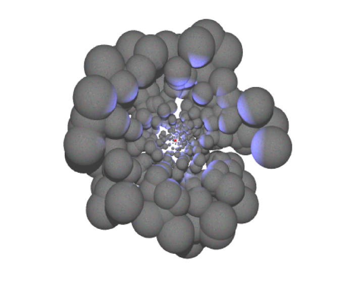
Figure 1: 3D rendering of the clump distribution of our standard clumpy torus model. The chosen inclination angle corresponds to a Seyfert 1 type (face-on) view onto the torus.

As in Nenkova et al. (2002), all clumps possess the same optical depth in our standard model. A total optical depth within the equatorial plane of $\left<\tau_{9.7\,\muup\mathrm{m}}^{\mathrm{equ}}\right>_{\phi}$ = 2.0 results in an optical depth of $\tau_{9.7\,\muup\mathrm{m}}^{\mathrm{clump}}=0.38$ along a radial ray through the centre of the clump. The corresponding continuous model has the same geometrical structure, continuously filled with dust according to the density distribution given in equation 1.

2.2 Summary of methods

A very brief overview of the dust composition, the heating source and the numerical method of radiative transfer will be given in this section.

Although several hints (Maiolino et al. 2001a, b; Jaffe et al. 2004) point to the possibility that dust in the nuclear regions of AGN is dominated by large grains, we will limit our present investigation to the classic MRN-model (Mathis et al. 1977) for three reasons: first, and most important, we aim for comparability with our earlier paper on continuous tori (Schartmann et al. 2005). Second, we have tested that our essential results about the change in grain size distribution (Sect. 3.9 in Schartmann et al. 2005) remain unchanged when distributing the dust in a clumpy structure. Third, our approach, which explicitly takes into account the size-dependent sublimation radius, is generically more robust against changes in the grain distribution than calculations that ignore this effect. For our current simulations, we represent the MRN-model by three different grain species with 5 different grain sizes each. Taking different sublimation radii of the various grains into account then partially accounts for the destruction of small grains in the harsh environment of the quasar, as they possess larger sublimation radii.

The dust distribution is heated by a point-like, central accretion disk with the SED of a mean quasar spectrum (see Fig. 3b in Schartmann et al. 2005). The radiation characteristic is chosen to follow a $|\cos(\theta)|$ law for all wavelengths. For the simulations shown in this paper, the accretion disk SED is normalised to a bolometric luminosity of $1.2\times 10^{11}\,L_{\sun}$, except for the comparison with the Circinus galaxy.

Figure 2: a) SEDs for a photon number study. The solid curves refer to our standard model and the dotted graphs (identical with the solid curves) result after doubling the number of photon packages. b) SEDs for a resolution study: high resolution (solid curves – our standard model) and a factor of 3 reduced number of grid cells (dotted curves). Shown are the cases for inclination angles $0\degr$ and $90\degr$.

In order to obtain the temperature, the SEDs and the surface brightness distributions of the dusty torus, we use the three-dimensional radiative transfer code MC3D (Wolf et al. 1999; Wolf 2003). We apply the Monte Carlo procedure mainly for the calculation of temperature distributions and the scattering part whenever necessary, whereas SEDs and surface brightness maps for dust reemission are obtained with the included raytracer. The main advantage compared to other codes is MC3D’s capability to cope with real three-dimensional dust density distributions, needed for a realistic modelling of the dust reemission from a clumpy torus. For this paper, we implemented the automatic determination of the sublimation surfaces of the various grain species in three dimensions. As we expect the sublimation to happen along irregularly shaped surfaces in a three dimensional, discontinuous model, a raytracing technique is used to solve the (1D) radiative transfer equation approximatively in all directions of the model space.

For further information on the radiative transfer procedure used and the other preconditions (mainly primary source and dust composition), see Wolf et al. (1999), Wolf & Henning (2000), Wolf (2001, 2003) and Schartmann et al. (2005).

2.3 Resolution study

In Fig. 2a, we show SEDs for our standard clumpy model (solid line, $5\cdot 10^{6}$ monochromatic photon packages) and for the same model, but with twice as many photon packages ($10^{7}$) used for the simulation of the temperature distribution (dotted graphs, identical with solid lines). Despite slight differences in the temperature distributions of single grains, we find an almost identical behaviour in the displayed SEDs, with differences smaller than the thickness of the lines. Maps at 12 $\mu$m display the same distribution with slight problems along the projected torus axis, which are not visible in the single surface brightness distributions and without any noticeable effect on the interferometric visibility distributions calculated from these maps. In Fig. 2b, the solid curves displays the SEDs for our high spatial resolution standard model and the dotted lines refer to a model with a factor of roughly three less grid cells. Only very small deviations are visible at short wavelengths. Fig. 2 clearly shows that the results and conclusions we draw from our simulations are neither affected by photon noise nor by too low spatial resolution.

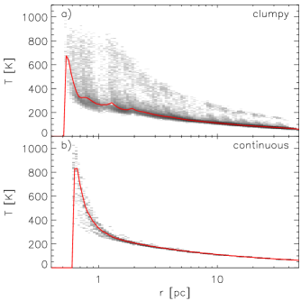
Figure 3: Comparison between radial temperature distributions (for the smallest silicate grains) in all directions of the clumpy standard model (panel a) with the temperature distribution of the corresponding continuous model (panel b). The red curve indicates the temperature averaged over all angles $\theta$ and $\phi$.

3 Analysis of our standard model

In most of the SEDs discussed in this paper, only pure dust reemission SEDs are shown and an azimuthal viewing angle of $45\degr$ is used, if not stated otherwise.

3.1 Temperature distribution

In Fig. 3, the temperature distribution of all cells in all $\theta$ and $\phi$ directions for the smallest silicate grain component is plotted a) for our clumpy standard model and b) for the corresponding continuous model. The red curves show the radial temperature profile, averaged over all $(\theta,\phi)$ directions. It is evident that the spread of temperature values for a given distance from the primary radiation source is much larger for the clumpy models than for the continuous ones. Higher temperatures are possible even in parts of the torus further out, as dust free or optically thin lines of sight exist far out, depending on the distribution of single clumps. Therefore, a direct illumination of clouds is possible even at large radii. Concerning the continuous model, the scatter decreases significantly from $2\,$pc outwards. Further in, the $\theta$ dependent radiation characteristic of the primary source causes greater scatter due to higher temperatures further away from the midplane.

3.2 Viewing angle dependence

Figure 4: Dependence of the SEDs on the viewing angle: a) different inclination angles for a common azimuthal angle $\phi$ $=$ $45\degr$. Inclination angles shown are: $0\degr$ (solid line), $30\degr$ (dotted line), $60\degr$ (dashed line), $90\degr$ (dashed-dotted line). b) Different azimuthal angles $\phi$ for a common inclination angle of $i=60\degr$. Azimuthal angles shown are: $0\degr$ (solid line), $45\degr$ (dotted line) and $180\degr$ (dashed line).

Fig. 4a shows the dependence of the spectral energy distributions on the inclination of the torus. One can only see a clear distinction between lines of sight within the dust-free funnel ($0\degr$ and $30\degr$ inclinations) and those within the wedge-shaped disk ($60\degr$ and $90\degr$). This was already reported by Granato & Danese (1994), based on their continuous wedge models. In our case, it is caused by the relatively large volume filling fraction and the large clouds in the outer part of the torus. Therefore, only a weak dependence of the dust density distribution on the polar angle exists, which we chose for simplicity. In our previous (2D) modelling (see Schartmann et al. 2005), we obtained the expected smooth transition in the polar direction. In Fig. 4b, the azimuthal angle is varied for a constant inclination angle of $60\degr$. Nearly identical SEDs result, which is understandable when considering our large volume filling factors. The largest deviations appear at the shortest wavelengths, where the emission results from the hottest parts of the torus, which are also the most centrally concentrated parts. Therefore, this wavelength range is most sensitive to changes of the optical depth along the direct line of sight towards the centre.

The dependence on the inclination angle of images is shown in Fig. 5 (upper two rows). It is especially interesting that the different inclination angles look very similar, which was not the case for the continuous model (see lower two rows of Fig. 5). There, the images at larger inclination angles are dominated by the boundaries of the disk, which are not so well defined in the clumpy case. In the zoomed-in images (Fig. 7, upper row), the basic features of our model are directly visible, as one can see the different illumination patterns of clouds: Clouds in the innermost part are fully illuminated and, therefore, show bright inner rims and cold outer parts. Other clouds are partly hidden behind clouds further in and appear as bright spots only.

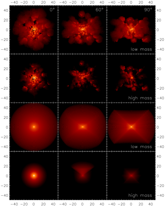
Figure 5: Inclination angle study of images of clumpy (first two rows) and continuous models (third and fourth row) with two different dust masses at $12\,\muup$m. Shown are the extreme cases with half of the mass of the standard model (first and third row) and eight times the mass (second and fourth row). For details of the mass study, see Sect. 4.3. The inclination angles $i=0\degr$, $60\degr$, $90\degr$ are shown in different columns. The scaling is logarithmic with a range between the maximum value of all images and the $10^{-6}$th fraction of it (excluding the central point source). Labels are sizes in pc.

3.3 Wavelength dependency

Fig. 6 shows the wavelength dependency of our standard model. At short wavelengths, the hottest inner parts dominate the brightness distribution. Further out, a few more directly illuminated clumps are visible as bright spots. At the longest wavelengths, emission arises from clumps all over the torus, as colder dust emits strongest at these wavelengths. This dust is spread over a larger volume, due to the steeply decreasing temperature distribution at small radii. Furthermore, the extinction curve has dropped by a large factor at these wavelengths and, therefore, the torus becomes optically thin and the whole range of cloud sizes is visible.

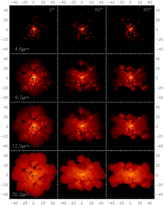
Figure 6: Wavelength dependence of the surface brightness distributions: $\lambda=4.6\,\muup$m (upper row), $\lambda=9.7\,\muup$m (second row), $\lambda=12.0\,\muup$m (third row) and $\lambda=30.2\,\muup$m (lower row). Within the rows, the inclination angle changes from face-on view (leftmost panel) over $60\degr$ to $90\degr$ (rightmost panel). The images are given in logarithmic scaling with a range of values between the global maximum of all images and the $10^{-5}\mathrm{th}$ fraction of it (central source excluded). Labels are in pc.

4 Parameter variations

4.1 Different realisations of the clumpy distribution

As already discussed in Schartmann et al. (2005), SEDs of dust reemission depend strongly on the distribution of dust in the innermost region. Changing the random arrangements of clumps – as done in this section – therefore is expected to cause significant changes of the SEDs, especially for the case of a small number of clouds. The second important parameter is the optical depth of the single clumps. The larger it is, the stronger is the dependence of the SEDs on the dust distribution in the innermost region. For the case of our modelling, the small number of clouds is expected to cause large differences in the observed SEDs. But this effect is partially compensated – in most of the simulations – by optically thin individual clumps, resulting in a more similar behaviour of the SEDs.

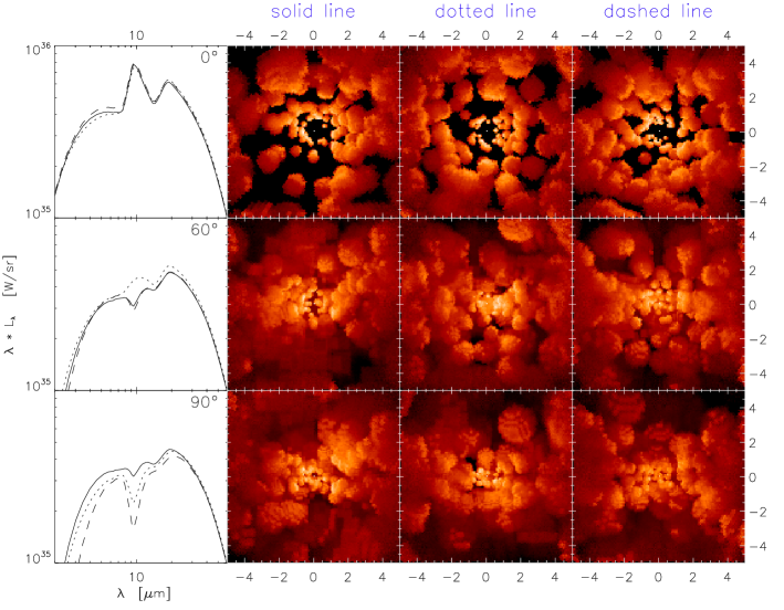
Figure 7: Different random arrangements of clumps. The rows show three different inclination angles: $0\degr$ (first row), $60\degr$ (second row), $90\degr$ (third row). Given in columns are the SEDs (first column) and the images at $12\,\muup$m for the three different random cloud arrangements (column 2 to 4), all having the same parameters (see Table 1). Here, the solid line in the SED corresponds to the first column of images, the dotted line to the second and the dashed line to the third column. Images are given in logarithmic color scale ranging from the maximum of all images to the $10^{-4}$th part of it (excluding the central source). Labels denote distance to the centre in pc.

Looking at the simulated SEDs and matching them with the images, the following results can be seen (compare to Fig. 7):

At $0\degr$ inclination angle (upper row), we observe nearly identical SEDs. The dashed line (corresponding to the fourth column) shows a slightly enhanced flux at short wavelengths, as a larger number of clouds are close to the central source. In the third column, the cloud number density in the central part is the lowest of the three examples.

For the case of the middle row ($i=60\degr$), the largest deviations are visible for the case of the dotted line (third column). Here, the silicate feature even appears in emission. This is visible in the surface brightness distributions, as more directly illuminated clouds are visible on unobscured lines of sight, resulting in a brighter central region compared to the other two maps. At an inclination angle of $90\degr$ (third row), absorption along the line of sight increases drastically from the second to the fourth column, visible in a deepening of the silicate absorption feature and the darkening of the central region of the surface brightness distributions.

4.2 Different volume filling factors

Starting from the standard model with a volume filling factor of $30\%$ and 400 clumps within the whole model space, we halved it once by distributing only 160 clumps within the calculation domain and doubled it, for which 1500 clumps were needed due to the applied procedure of randomly distributing clumps.

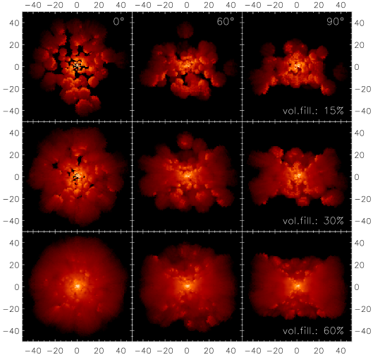
Figure 8: Different volume filling factors: $15\%$ (upper row), $30\%$ (middle row), $60\%$ (lower row) for $\lambda=12.0\,\muup$m. From left to right, the inclination angle changes: $i=0\degr$, $60\degr$, $90\degr$. The scaling is logarithmic with a range between the maximum value of all images and the $10^{-6}$th fraction of it (excluding the central point source). Length scales are given in pc.

Figure 9: Different volume filling factors: $15\%$ (dotted line), $30\%$ (solid line), $60\%$ (dashed line). Rows show SEDs for the three inclination angles: $i=0\degr$, $60\degr$, $90\degr$. The viewing angle in $\phi$-direction is always $45\degr$.

The resulting surface brightness distributions at $\lambda\,=\,12.0\,\muup$m are shown in Fig. 8 with the three models given in different rows and for three different inclination angles: $i=0\degr$, $60\degr$, $90\degr$. In the case of the lowest volume filling factor, individual clouds are visible. The distribution of the surface brightness of these individual clouds reflects the temperature structure within single clumps. The directly illuminated clumps are hotter and, therefore, appear brighter. When adding more and more clumps (increasing the volume filling factor), the chance of directly illuminating clumps further out decreases and at higher filling factors it is only possible for clumps close to the funnel. This is clearly visible at higher inclination angles: the higher the volume filling factor, the clearer the x-shaped feature appears, as only clumps within or close to the funnel can be directly illuminated. At a volume filling factor of $60\%$, the surface brightness distribution looks very similar to that of the corresponding continuous model (compare to Fig. 5). For large volume filling factors and close to edge-on, substructure is only visible from clouds in a viewing direction towards the dust-free cones.

The corresponding SEDs are shown in Fig. 9. With increasing filling factor, more and more flux at short wavelengths appears for the face-on case, as seen in Schartmann et al. (2005). The shape of the clumpy model SEDs resemble the corresponding continuous model most (compare to Fig. 10, right column) for the highest volume filling factor. Concerning the silicate feature, it increases slightly in emission as the amount of dust at the appropriate temperature increases as well (visible at the transition from the lowest to the medium volume filling factor). The silicate absorption feature at higher inclinations strongly depends on the viewing angle (compare Fig. 9b and c) especially for the model with the least number of clumps (dotted line). Thus, this study shows the validity of the simplification of using a smooth dust distribution in the case of very high torus volume filling factors, as was assumed in previous simulations.

4.3 Dust mass study

To study the dependence of the SEDs on the optical depth of the torus, we carried out a study with 0.5, 1, 2, 4 and 8 times the dust mass in the standard model. This leads to an optical depth at 9.7$\,\muup$m within the equatorial plane, averaged over all angles of $\phi$ of $\left<\tau_{9.7\,\muup\mathrm{m}}^{\mathrm{equ}}\right>_{\phi}=$ 1, 2, 4, 8, 16. Single clumps then change from optically thin to optically thick ($\tau_{9.7\,\muup\mathrm{m}}^{\mathrm{clump}}=0.19,0.38,0.76,1.52,3.04$).

Figure 10: SEDs for different enclosed dust masses. The left column shows the case for the clumpy models and a face-on view (upper row) as well as an edge-on view (lower row). In the right column, continuous models are displayed. The solid line corresponds to the standard model, the dotted to half of the mass, the dashed double the mass, the dash-dotted to four times the mass and the dash-triple-dotted to eight times the mass of the standard model.

Figure 11: Close-up of the spectrum between 7 and $15\,\muup$m of the face-on case of the dust mass study for the clumpy model in linear display. The lines are defined as in Fig. 10.

The resulting behaviour of the SEDs is shown in Fig. 10, where it is also compared to the corresponding continuous models. Concerning the silicate feature (in emission) for the face-on case (top row), we see a very similar behaviour of the SEDs of the clumpy and continuous model. Increasing the mass and with it the total optical depth leads to a flattening of the SED around the silicate feature, even more pronounced in the continuous case. In addition to that, a slight shift of the maximum of the silicate feature towards longer wavelengths is visible for the case of the highest dust mass, apparent in the zoom-in of Fig. 10 around the silicate feature (see Fig. 11). This is due to the increasing underlying continuum towards longer wavelengths. Although the principal behaviour of the silicate feature is identical for our clumpy and our continuous model, the reasons differ: In the case of a continuous wedge-like torus, the inner, directly illuminated walls are only visible through a small amount of dust. From step to step, the walls become more opaque and shield the directly illuminated inner rim better, decreasing the height of the silicate feature. This was not the case for our continuous TTM-models in Schartmann et al. (2005). With them, it was not possible to significantly reduce the silicate feature height within reasonable optical depth ranges. This was caused by the fully visible, directly illuminated inner funnel. Therefore, in the wedge-shaped continuous models, the reduction of the feature is an artefact caused by the unphysical, purely geometrically motivated shape. Furthermore, it also involves very deep and so far unobserved silicate absorption features for the edge-on case (see lower right panel in Fig. 10). Concerning the clumpy model, the explanation for the flattening of the silicate feature in the edge-on case with increasing dust mass of the torus will be given in Sect. 5.1.

The Wien branches show different behaviour when looking face-on. For the case of the clumpy torus model, increasing the optical depth means that the Wien branch moves to larger wavelengths, as expected for the edge-on case. This is understandable when most of the directly illuminated surfaces of the clouds are then hidden behind other clouds, an argument which is not valid if the clouds are too optically thin in the inner part.
For the edge-on case, we qualitatively obtain a comparable behaviour as in the continuous case, because of the large number of clumps and the same optical depth within the equatorial plane. But a very important difference can be seen in the appearance of the silicate feature in absorption: when we want to have only very weak silicate emission features in the face-on case, a large optical depth is needed, resulting in an unphysically deep silicate feature in absorption in the edge-on case of the continuous models, whereas the silicate feature remains moderate for many lines of sight for the clumpy model, where we see a large scatter for different random arrangements of clumps (compare to Fig. 7).

Concerning surface brightness distributions (see Fig. 5), one can see that the objects appear smaller at mid-infrared wavelengths for the case of higher dust masses: the larger the optical depth, the brighter the inner region and the dimmer the outer part. This is caused by a steepening of the radial dust temperature distribution with increasing mass of the objects, as the probability of photon absorption increases in the central region. Especially for the continuous case, the asymmetry at intermediate inclination angles becomes visible for larger optical depths caused by extinction on the line of sight due to cold dust in the outer parts of the torus.

4.4 Concentration of clumps in radial direction

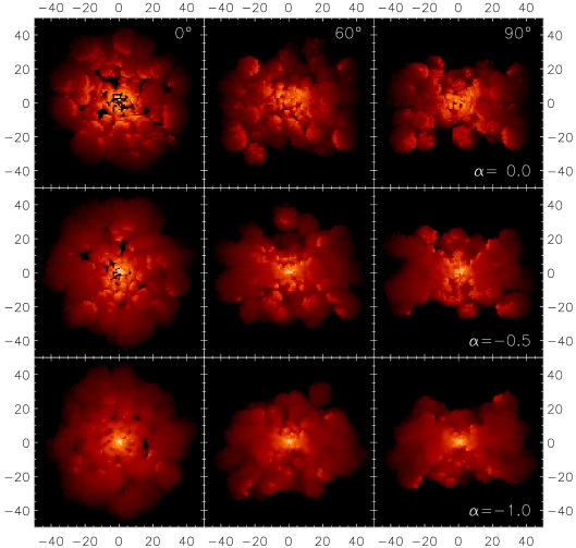
Figure 12: Surface brightness distributions for various slopes of the density distribution in the corresponding continuous model ($\rho_{\mathrm{cont}}\propto r^{\alpha}$) leading to different concentrations of clumps in the radial direction in the clumpy model. The slopes are: $\alpha=0.0$ (upper row), $\alpha=-0.5$ (middle row), $\alpha=-1.0$ (lower row). From left to right, the inclination angle increases from face-on to edge-on: $i=0\degr$, $60\degr$, $90\degr$. Shown are images at $12\,\muup$m with a logarithmic color scale ranging from the maximum of all images to the $10^{-6}$th part of it. Labels denote the distance to the centre in pc.

As already described in the model section (2), clump positions are also chosen in accordance with the density distribution of the corresponding continuous model. Therefore, changing the slope of this radial density distribution, defined to be $\rho_{\mathrm{cont}}(r,\theta,\phi)=\rho_{0}\,\left(\frac{r}{1\,\mathrm{pc}}\right)^{\alpha}$, leads to a different concentration of clumps along radial rays. In this section, we vary the slope of the distribution $\alpha$ from a homogeneous dust distribution ($\alpha=0.0$) over $\alpha=-0.5$ (our standard model) to $\alpha=-1.0$. Decreasing $\alpha$ leads to an enhancement of the clump number density towards the central region. In order to keep the volume filling fraction at a constant level of $30\%$, we need to increase the number of clumps, as their size decreases towards the central region. All clumps possess the same optical depth. In order to have a constant mean optical depth in the midplane, the total dust mass has to be decreased. For an overview of the modified parameters see Table  2.

Table 2: Varied parameters of the clump concentration study.

Parameter	$\alpha=0$	$\alpha=-0.5$	$\alpha=-1$
No. of clumps	250	400	900
Dust mass [$\mathrm{M}_{\sun}$]	22950	12562	6418

The change of clump concentration can be seen directly from the simulated images at $12.0\,\muup$m in Fig. 12, especially in the face-on case (first column). In the upper panel, single reemitting clumps are visible in the central region. This changes more and more to a continuous emission for the case of the highest cloud concentration in the centre due to multiple clumps along the line of sight and intersecting clumps. At higher inclination angles, the higher concentration leads to a sharper peak of the surface brightness.

The same behaviour is visible in the corresponding SEDs shown in Fig. 13. Decreasing the amount of dust in the centre near the heating source leads to decreasing flux at near-infrared wavelengths, whereas the flux at far-infrared wavelengths increases (reflecting the enhancement of dust in the outer part).

Figure 13: SEDs for the clump concentration study. The varied slopes of the underlying density distribution are: $\alpha=0.0$ (dotted line), $\alpha=-0.5$ (solid line), $\alpha=-1.0$ (dashed line): a) face-on, b) edge-on.

4.5 Dependence on the clump size distribution

In our clumpy standard model, a radially changing clump size proportional to the radial distance to the centre was chosen. In this section, we test the effects of decreasing the slope $\beta$ of the radial size distribution $a_{\mathrm{clump}}=a_{0}\,\left(\frac{r_{\mathrm{clump}}}{1\,\mathrm{pc}}\right)^{\beta}$ of the clumps. This is done in a way that the volume filling fraction as well as the optical depth in the midplane, averaged over all azimuthal angles $\phi$, remain constant. It is achieved by changing the proportionalisation constant of the clump size distribution $a_{0}$ and the total dust mass of the torus. Doing this results in very well resolved clumps in the inner part. Beyond a distance of approximately $25\,$pc, the number of grid cells per clump drops below the value of our standard model.

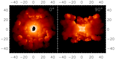
Figure 14: Images at $12\,\muup$m and inclination angles $i=0\degr$ and $90\degr$ for a clumpy distribution with a constant clump size, independent of the radial position. The scaling is logarithmic with a range between the maximum value of all images and the $10^{-6}$th fraction of it (excluding the central point source).

Surface brightness distributions for the extreme case of a constant clump size are shown in Fig. 14. Due to the large clump radius of $5\,$pc even in the central region and that fractions of clumps at the model space boarder are prohibited, it leads to a density distribution with a quite large, unevenly shaped central cavity, as can be seen in the face-on view (left panel of Fig. 14). The inner rim is given by only a few intersecting clumps, instead of the otherwise defined spherical central cavity. Therefore, in the edge-on case, the surface brightness distribution shows an inner boundary, which is bent towards the centre (convex shaped). In these models, due to the large clump size in the inner region, many clumps intersect, producing a nearly continuous dust distribution at the inner boundaries, which lets the – typical for continuous models – x-shaped structure appear again. For the same reason, the extinction band due to the $|\cos(\theta)|$-radiation characteristic is visible in the edge-on view. Especially at the $90\degr$ inclination angle, single clumps are directly visible (above and below the centre). In these cases, their shading directly shows the illumination pattern due to the primary source (accretion disk), emission from other clumps and extinction from the foreground dust distributions.

Figure 15: Dependence on the clump size for different inclination angles (rows: $0\degr$, $60\degr$, $90\degr$). The solid line corresponds to our standard model with $\beta=1$. For the dashed line, clumps have equal size ($a_{\mathrm{clump}}=5\,$pc, $\beta=0$), independent of the radial position and the dotted line corresponds to an intermediate model with $\beta=0.5$.

The corresponding SEDs (Fig. 15) mainly reflect the increase of the inner cavity and, therefore, the lack of flux at short wavelengths. The convex shape of that region causes a larger directly illuminated area at the funnel walls and, therefore, slightly strengthens the silicate emission feature in a face-on view. A different appearance (emission/absorption) of the $10\,\muup$m feature at $i=60\degr$ (middle panel) is seen. This is due to the lower number density of clumps in the inner part, enforced by the restriction of having only whole clumps within the model space.

A dust mass study for the case of the large, constant diameter clump model ($\beta=0$) reveals the same behaviour as discussed in Sect. 4.3 when looking edge-on onto the torus. However, the face-on case differs: only the relative height of the silicate feature changes slightly. This was already observed in our TTM-models in Schartmann et al. (2005) and is due to the now inwardly bent inner walls of the funnel (see Fig. 14, right panel), caused here by the very large and spherical clumps in the innermost torus region.

5 Discussion

5.1 Explanation for the reduction of the silicate feature

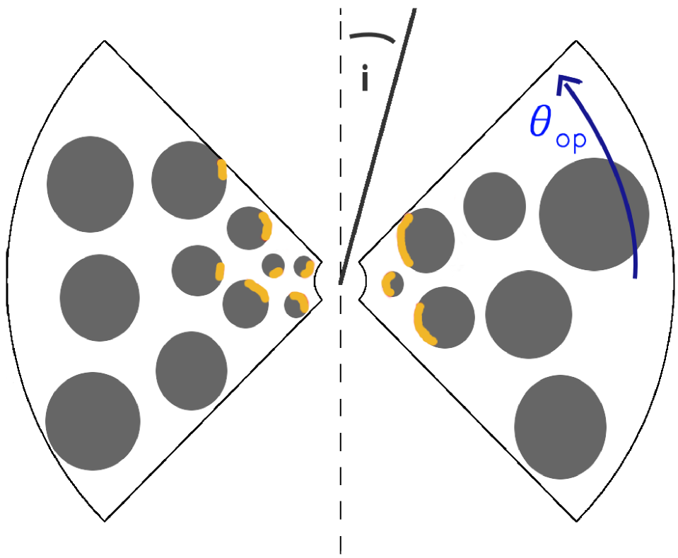
Figure 16: Sketch of our clumpy torus model. Indicated in yellow are directly illuminated surfaces of the clumps. $i$ is the inclination angle, $\theta_{\mathrm{open}}$ is the half opening angle of the torus.

The results shown in the subsections before can be explained with the following model, which was partially discussed by Nenkova et al. (2002). It is illustrated in Fig. 16, where yellow denotes directly illuminated clump surfaces. Many of the explained features can also be seen in the zoomed-in versions of the surface brightness distributions (Fig. 7) for the face-on case (upper row).

As already pointed out in Schartmann et al. (2005), the SEDs of dust tori in the mid-infrared wavelength range are mainly determined by the inner few parsecs of the toroidal dust distribution. In each of the central clouds of the clumpy model, the dust temperature drops from the inner directly illuminated edge towards the cloud’s outer surface.

With an inclination angle close to $i=90\degr$, we expect – for realistic volume filling factors – comparable behaviour of the SED as in the continuous case. The silicate feature has a smaller depth, as discussed in Sect. 4.3. But the situation changes with decreasing inclination angle. Here, one has to distinguish between different cases:

1. With a relatively high volume filling factor and a not too small extension of the clouds in the central region of the torus, it is likely that the directly illuminated part of most of the clouds is hidden from direct view by other clouds. Therefore, the directly illuminated surface area is reduced compared to the corresponding continuous model. As this area is responsible for the emission fraction of the silicate feature within the SED, it shows less silicate emission. In order to produce such a shadowing effect, clouds have to possess a large enough optical depth, which means that they have to be either small or massive ($\tau_{\mathrm{clump}}\propto m_{\mathrm{clump}}\,a_{\mathrm{clump}}^{-2}$, where $m_{\mathrm{clump}}$ is the mass of the clump).

2. For the case of a too small optical depth of the clumps in the innermost region, we expect the silicate feature to appear in strong emission.

3. Another possibility of producing silicate features in emission is when the model possesses a small number of clumps in the inner part, making the shadowing effect inefficient.

4. A further effect on the silicate feature strength arises from the grain dependent sublimation implemented in our models. As graphite grains possess a higher sublimation temperature as silicate grains, they are able to partially shelter the silicate grains from direct irradiation.

Thus, the strength of the silicate feature is mainly determined by the distribution, size and optical depth of the clouds in the direct vicinity of the sublimation surface of the dust. We will see in the next section that this finding well explains the fact that Nenkova et al. (2002) and Dullemond & van Bemmel (2005) come to different conclusions concerning the reduction of the strength of the silicate feature due to clumpiness, as the distribution (and size) of their clouds differ.

5.2 Comparison with other torus models

The results of Nenkova et al. (2002) - the pioneering work in the field of clumpy tori - are broadly consistent with the explanations given in Sect. 5.1 of this paper.

Dullemond & van Bemmel (2005) model 2D clumps in the form of rings with a two-dimensional radiative transfer code. In contradiction to all other simulations, no systematic reduction of the silicate feature due to clumpiness is found. The reason for this is understandable with the explanations given in Sect. 5.1, as their model features a small clump number density in the central region and shadowing effects are rather small. Therefore, they find both strengthening of the silicate feature and reduction, depending on the random ring distribution.

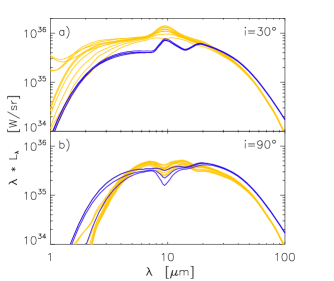
Figure 17: Comparison of our clumpy standard model and two other random realisations of the clump distribution (blue lines) with simulations done by S. F. Hönig (private communication, described in Hönig et al. 2006), shown by the yellow lines, for 10 different random realisations of their model. The latter are scaled with a factor of 2.2 in order to give rough agreement between the two models (see text for further explanation).

A comparison of our clumpy standard model and two other random cloud distributions with simulations by Hönig et al. (2006) is shown in Fig. 17. They follow a different, multi-step approach: 2D radiative transfer calculations of individual clouds at different positions and with various illumination patterns within the torus are carried out. In a second step, the SED of the total system is calculated. The cloud distribution and parameters such as optical depth or size arise from an accretion scenario of self-gravitating clouds close to the shear limit (Vollmer et al. 2004; Beckert & Duschl 2004). The advantage of this approach is that resolution problems can be overcome easily, as only 2D real radiative transfer calculations of single clumps are needed. Characteristics for their modelling are small cloud sizes with very high optical depths in the inner part of the torus and a large number of clumps. For comparison, a cloud at the sublimation radius of their model has a radial size of $R_{\mathrm{cloud}}=0.02\,$pc with an optical depth of $\tau_{0.55\,\muup\mathrm{m}}^{\mathrm{clump}}\approx 250$. In our standard model, clouds at the sublimation radius are four times larger and possess an optical depth of only $\tau_{0.55\,\muup\mathrm{m}}^{\mathrm{clump}}\approx 3$. The large optical depth in the innermost part in combination with the large number density there reduces the silicate feature significantly by shadowing with respect to their single clump calculations. Their finding that the silicate emission feature can be reduced further by increasing the number density of clumps in the innermost part perfectly fits our explanation presented in Sect. 5.1. Deviations between the two approaches (see Fig. 17) are mainly due to the approximately eight times larger primary luminosity and the larger optical depth, at least in the midplane of the Hönig et al. (2006) modelling compared to our standard model. Furthermore, in our simulations only dust reemission SEDs are shown. This leads to relatively higher fluxes at short wavelengths compared to long wavelengths for the $i=30\degr$ case (Fig. 17a) and to more extinction within the midplane and, therefore, a shift of the Wien branch towards longer wavelengths in the edge-on case (lower panel).

6 MIDI interferometry

Even with the largest single-dish mid-infrared telescopes, it is impossible to directly resolve the dust torus of the nearest Seyfert galaxies. Therefore, interferometric measurements are needed. Recently, Jaffe et al. (2004) succeeded for the first time to resolve the dusty structure around an AGN in the mid-infrared wavelength range. In this case, they probed the active nucleus of the nearby Seyfert 2 galaxy NGC 1068 with the help of the MID-infrared interferometric Instrument (MIDI, Leinert et al. 2003). It is located at the European Southern Observatory’s (ESO’s) Very Large Telescope Interferometer (VLTI) laboratory on Cerro Paranal in Chile. Its main objective is the coherent combination of the beams of two 8.2 m diameter Unit Telescopes (UTs) in order to obtain structural properties of the observed objects at high angular resolution. A spatial resolution of up to $\lambda/(2\,B)\approx 10\,$mas at a wavelength of $\lambda=10\,\muup$m can be obtained for the largest possible separation of two Unit Telescopes of $B\approx 120\,$m. Operating in the N-band ($8-13.5\,\muup$m), it is perfectly suited to detect thermal emission of dust in the innermost parts of nearby Seyfert galaxies. MIDI is designed as a classical Michelson interferometer. Being a two-element beam combining instrument, it measures so-called visibility amplitudes. Visibility is defined as the ratio between the correlated flux and the total flux. Its interpretation is not straightforward, since no direct image can be reconstructed. Therefore, a model has to be assumed, which can then be compared to the visibility data.

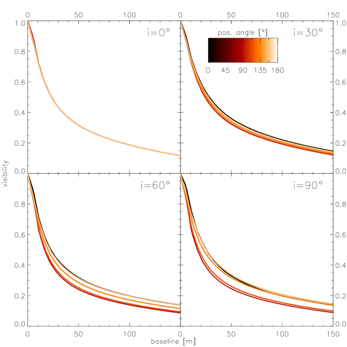
Figure 18: Visibilities of our continuous standard model at a wavelength of $12\,\muup$m plotted against the projected baseline length. Colour of the visibility distributions refers to different position angles of the projected baseline w. r. t. the torus axis. Each panel shows a different inclination angle, as indicated in the upper right corner.

MIDI works in dispersed mode, which means that visibilities for the whole wavelength range are derived. The dust emission is probed depending on the orientation of the projected baseline. Point-like objects result in a visibility of one, as the correlated flux equals the total flux. The more extended the object, the lower the visibility. With the help of a density distribution, surface brightness distributions in the mid-infrared can be calculated by applying a radiative transfer code. A Fourier transform of the brightness distribution then yields the visibility information, depending on the baseline orientation and length within the so-called U-V-plane (or Fourier-plane).

The main goal of the following analysis is to investigate whether MIDI can distinguish between clumpy and continuous torus models of the kind presented above. Furthermore, we try to derive characteristic features of the respective models and show a comparison to data obtained for the Circinus galaxy.

6.1 Model visibilities

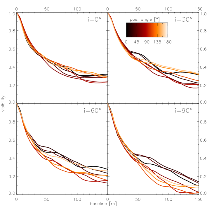
Figure 19: Visibilities of our clumpy standard model at a wavelength of $12\,\muup$m plotted against the projected baseline length. Colour of the visibility distributions refers to different position angles of the baseline w. r. t. the torus axis. Each panel shows a different inclination angle, as indicated in the upper right corner.

In Fig. 18, calculated visibilities for four inclinations of our continuous standard model at a wavelength of $\lambda$ $=$ $12\,\muup$m are shown. Various orientations of the projected baseline are colour coded (the given position angle is counted anti-clockwise from the projected torus axis). Due to the axisymmetric setup, all lines coincide for the face-on case. For all other inclination angles, visibilities decrease until a position angle of $90\degr$ is reached and increase symmetrically again. This means that the torus appears elongated perpendicular to the torus axis at this wavelength. Fig. 19 shows the same study, but for the corresponding clumpy model. The basic behaviour is the same, but the visibilities show fine structure and the scatter is much greater, especially visible in the comparison of the $i=0\degr$ cases. Furthermore, while all of the curves of the continuous model monotonically decrease with baseline length, we see rising and falling values with increasing baseline length for the same position angle in the clumpy case. In addition, for the continuous models, curves do not intersect, in contrast to our clumpy models. However, to detect such fine structure in observed MIDI data, a very high accuracy in the visibility measurements of the order of $\sigma_{v}\approx 0.02$ and a very dense sampling is required.

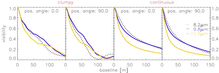
Figure 20: Visibilities of our clumpy (first two panels) and continuous (last two panels) standard model at different wavelengths (colour coded), plotted against the projected baseline length for the two position angles $0\degr$ (in torus axis direction) and $90\degr$ (along the midplane) for an edge-on view onto the torus ($i=90\degr$).

In Fig. 20, the wavelength dependence of the visibilities is shown. The first two panels represent the case of the clumpy standard model and the third and fourth the continuous model. Each of the two panels of the respective model visualises a different position angle (counted anti-clockwise from the projected torus axis). An inclination angle of $90\degr$ is used in all panels. Three different wavelengths are colour coded: $8.2\,\muup$m at the beginning of the MIDI-range (black dotted line), $9.8\,\muup$m within the silicate feature (blue) and $12.6\,\muup$m at the end of the MIDI wavelength range (yellow), outside the silicate feature. While the continuous model results in smooth curves (see also Fig. 18), much fine structure is visible for the case of the clumpy model. The differences between the displayed wavelengths relative to the longest wavelength are smaller for the clumpy models than in the continuous case.

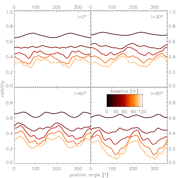
Figure 21: Visibilities of our clumpy standard model at different inclination angles (as annotated in the upper right corner) plotted against the position angle for various projected baseline lengths (colour coded) and a wavelength of $12\,\muup$m.

Fig. 21 shows visibilities for our clumpy standard model at $12\,\muup$m, plotted against the position angle (counter-clockwise from the projected torus axis). Baselines are colour coded between $20\,$m and $100\,$m in steps of $20\,$m. A longer baseline means that structures are better resolved, leading to decreasing visibilities. For the case of inclination angles close to edge-on, the visibility distribution changes from more or less flat to a characteristic oscillating distribution at longer baselines (from $60\,$m onwards) with minima around $100\degr$ and $300\degr$. This means that our torus model seems to be more elongated within the equatorial plane and has the smallest width along the projected torus axis at this wavelength. But this only applies for the innermost part; the torus as a whole looks approximately spherically symmetric. At small inclination angles no such favoured size distribution is visible.

6.2 Comparison with MIDI-data for the Circinus galaxy

Table 3: Circinus model parameters: For an explanation of the parameters see Sect. 2 and Table 1. $M_{\mathrm{BH}}$ is the mass of the central black hole (from Greenhill et al. 2003) and $L_{\mathrm{disk}}/L_{\mathrm{edd}}$ is the Eddington luminosity ratio resulting for the assumed luminosity of the central source.

Parameter	Value		Parameter	Value
$R_{\mathrm{in}}$	0.6 pc		$N_{\mathrm{clump}}$	500
$R_{\mathrm{out}}$	30 pc		$\beta$	1.0
$\theta_{\mathrm{open}}$	$65\degr$		$a_{0}$	0.2 pc
$\left<\tau_{9.7\,\muup\mathrm{m}}^{\mathrm{equ}}\right>_{\phi}$	3.9		$\tau_{9.7\,\muup\mathrm{m}}^{\mathrm{clump}}$	0.96
$M_{\mathrm{BH}}$	$1.7\cdot 10^{6}\,M_{\sun}$		$L_{\mathrm{disk}}/L_{\mathrm{edd}}$	30%
$\alpha$	-0.5

Unfortunately, a fitting procedure involving a large parameter study is not possible with our current model, due to the very long computational times of the order of 30 to 40 hours per inclination angle (including calculation of the temperature distribution, the SED and surface brightness distribution). Therefore, we applied the following procedure: From our experience with modelling the SED of the Circinus galaxy with our previously used continuous Turbulent Torus Models (see Schartmann et al. 2005), we adopt the size of the object used there. Furthermore, we tried to stay as close to our clumpy standard model as possible (for the parameters of the clumpy standard model, compare to Table 1) and copied the parameters $\alpha$, $\beta$ and $a_{0}$. The rest of the parameters were changed, in order to obtain the best possible adaptation to the data, within the investigated parameter range. The comparison of our current clumpy Circinus model as described above and in Table 3 (yellow stars) to interferometric observations with MIDI (Tristram et al. 2007) of the Circinus galaxy (black) is shown in Fig. 23. In contrast to the presentation of continuous visibility curves above, single measurements of combinations of various baseline lengths and position angles are displayed in this plot. Position angle now refers to the angle on the sky measured from north in a counter-clockwise direction. The rotation axis of our simulated torus has a position angle of approximately $-45\degr$ according to this definition. The black numbers denote the length of the projected baseline (given in m) of the corresponding data point. From the approximate correspondence of the model values with the data, one can see that the size of the emitting region at the two wavelengths is reproduced quite well. Most of the local extrema of the curve can be reproduced for the case of $9.1\,\muup$m. Larger deviations are visible for $\lambda=12.0\,\muup$m. The good adaptation partly is due to the changes in baseline length. Longer baselines naturally result in smaller visibilities, as we are probing smaller and smaller structures (see also Fig. 19). Greater visibilities for shorter or equal baselines and similar position angle, therefore, have to be due to those curves in Fig. 19 with increasing visibility with baseline or a very inhomogeneous distribution of dust with position angle. Both can be interpreted as signs of clumpiness. The SED of the same Circinus model is plotted over current high resolution data in Fig. 23. The NIR (near-infrared) data points were obtained with the NACO camera at the VLT and corrected for foreground extinction by $A_{\mathrm{V}}=6\,$mag (Prieto et al. 2004). Different symbols refer to various aperture sizes (see figure caption). The thick green line shows the MIDI spectrum (Tristram et al. 2007) and the black line is our Circinus model as discussed above for an aperture of $0.4\arcsec$ in radius; the yellow line denotes the same model, but calculated for the whole simulated model space. Both modelled SEDs include the direct radiation of the central source (calculated with real Monte Carlo radiative transfer), which in these examples dominates over dust reemission for the small wavelength part from about 2 to $3\,\muup$m downwards and shows some noise, due to the low photon packet numbers used. In contradiction to our continuous Circinus model in Schartmann et al. (2005), enough nuclear radiation can be observed in order to explain the turnover of the SED at small wavelengths and we do not need to assume scattering by material (dust and electrons) within the torus funnel. As can be seen from these figures, our model is able to qualitatively explain the SED as well as the visibility information. However, as we are not able to investigate the whole parameter range of our models, we cannot exclude that a different parameter set can describe the data equally well. This degeneracy problem was already pointed out by Galliano et al. (2003) for the case of SED fitting. Adding new clumpiness parameters will even strengthen this degeneracy. On the other hand, adding more data such as more visibility information will place more constraints and will weaken this problem.

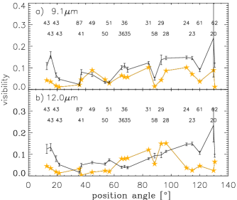
Figure 22: Comparison of model visibilities (yellow stars and lines) for an azimuthal viewing angle of $\phi=225\degr$ with MIDI observations for two different wavelengths. The baseline length for all data points is given above the data. Data courtesy of Tristram et al. (2007).

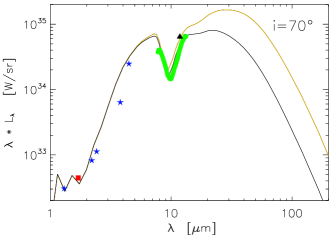
Figure 23: Comparison of model SEDs with data for the Circinus galaxy. Different symbols refer to various aperture radii: blue stars – $0.38\arcsec$ (NACO), red rectangle – $0.1\arcsec$ (HST/NICMOS) and black triangle – $1.0\arcsec$ (ESO/TIMMI2). Data compilation by Prieto et al. 2004. The thick green line shows the total MIDI spectrum (Tristram et al. 2007). Our model (see model parameters in Table 3) is calculated for an aperture radius of $0.4\arcsec$ (black line) and the total model space (yellow line).

7 Conclusions

In this paper, we implemented a new clumpy torus model in three dimensions. For computational reasons, a wedge-like shaped disk is used. In the discussion of our results, we place special emphasis on the comparison with continuous models and their differentiation using interferometric observations, such as with MIDI.

In Schartmann et al. (2005), we had found that the SEDs of AGN tori in the mid-infrared wavelength range are mainly determined by the innermost part of the torus. With the presented clumpy torus models, this claim can be further strengthened. According to the new simulations, the silicate feature strength is mainly determined by the number density and distribution, as well as the optical depth and size of the clumps in the inner region. With a sufficiently high optical depth of the clouds in the inner part, shadowing effects become important, which hide the illuminated cloud surfaces from direct view and, thereby, reduce the silicate feature in emission. At the same time, enough lines of sight with low optical depth remain so that only weak absorption features result for the edge-on case. Continuous models with special and unrealistic morphologies (like the wedge-shaped tori used here) are also able to weaken the silicate emission feature for the face-on view when applying an anisotropic radiation characteristic, but fail to simultaneously account for moderate absorption features, when looking edge-on to the torus.

Due to the large clumps in our model, appreciable scatter in SEDs for different random realisations of the torus are expected. A contrary effect is caused by the small optical depth of the single clumps and also of many dust-free lines of sight towards the centre. Direct comparison between calculated interferometric visibilities for clumpy and the corresponding continuous models show that clumpy models naturally possess more fine structure, which can partly be resolved by MIDI.

We also showed that these kinds of models are able to qualitatively describe the available interferometric visibility and high resolution spectroscopic data of the Circinus galaxy at the same time. Currently, it is one of the best studied Seyfert galaxies in terms of mid-infrared visibility measurements (Tristram et al. 2007). The decreasing slope of the SED at short wavelengths can be described with our clumpy model, whereas it was at odds with the continuous model described in Schartmann et al. (2005).