Guarding curvilinear art galleries with vertex or point guards

Abstract

One of the earliest and most well known problems in computational geometry is the so-called art gallery problem. The goal is to compute the minimum possible number guards placed on the vertices of a simple polygon in such a way that they cover the interior of the polygon.

In this paper we consider the problem of guarding an art gallery which is modeled as a polygon with curvilinear walls. Our main focus is on polygons the edges of which are convex arcs pointing towards the exterior or interior of the polygon (but not both), named piecewise-convex and piecewise-concave polygons. We prove that, in the case of piecewise-convex polygons, if we only allow vertex guards, $\lfloor\frac{4n}{7}\rfloor-1$ guards are sometimes necessary, and $\lfloor\frac{2n}{3}\rfloor$ guards are always sufficient. Moreover, an $O(n\log{}n)$ time and $O(n)$ space algorithm is described that produces a vertex guarding set of size at most $\lfloor\frac{2n}{3}\rfloor$. When we allow point guards the afore-mentioned lower bound drops down to $\lfloor\frac{n}{2}\rfloor$. In the special case of monotone piecewise-convex polygons we can show that $\lfloor\frac{n}{2}\rfloor$ vertex guards are always sufficient and sometimes necessary; these bounds remain valid even if we allow point guards.

In the case of piecewise-concave polygons, we show that $2n-4$ point guards are always sufficient and sometimes necessary, whereas it might not be possible to guard such polygons by vertex guards. We conclude with bounds for other types of curvilinear polygons and future work.

1 Introduction

Consider a simple polygon $P$ with $n$ vertices. How many points with omnidirectional visibility are required in order to see every point in the interior of $P$? This problem, known as the art gallery problem has been one of the earliest problems in Computational Geometry. Applications areas include robotics [20, 35], motion planning [23, 27], computer vision and pattern recognition [31, 36, 2, 32], graphics [25, 7], CAD/CAM [4, 15] and wireless networks [16]. In the late 1980’s to mid 1990’s interest moved from linear polygonal objects to curvilinear objects [34, 9, 11, 10] — see also the paper by Dobkin and Souvaine [13] that extends linear polygon algorithms to curvilinear polygons, as well as the recent book by Boissonnat and Teillaud [3] for a collection of results on non-linear computational geometry beyond art gallery related problems. In this context this paper addresses the classical art gallery problem for various classes of polygonal regions the edges of which are arcs of curves. To the best of our knowledge this is the first time that the art gallery problem is considered in this context.

The first results on the art gallery problem or its variations date back to the 1970’s. Chvátal [8] was the first to prove that a simple polygon with $n$ vertices can be always guarded with $\lfloor\frac{n}{3}\rfloor$ vertices; this bound is tight in the worst case. The proof by Chvátal was quite tedious and Fisk [18] gave a much simpler proof by means of triangulating the polygon and coloring its vertices using three colors in such a way so that every triangle in the triangulation of the polygon does not contain two vertices of the same color. The algorithm proposed by Fisk runs in $O(T(n)+n)$ time, where $T(n)$ is the time to triangulate a simple polygon. Following Chazelle’s linear-time algorithm for triangulating a simple polygon [5, 6], the algorithm proposed by Fisk runs in $O(n)$ time. Lee and Lin [21] showed that computing the minimum number of vertex guards for a simple polygon is NP-hard, which was extended to point guards by Aggarwal [1]. Soon afterwards other types of polygons were considered. Kahn, Klawe and Kleitman [19] showed that orthogonal polygons of size $n$, i.e., polygons with axes-aligned edges, can be guarded with $\lfloor\frac{n}{4}\rfloor$ vertex guards, which is also a lower bound. Several $O(n)$ algorithms have been proposed for this variation of the problem, notably by Sack [29], who gave the first such algorithm, and later on by Lubiw [24]. Edelsbrunner, O’Rourke and Welzl [14] gave a linear time algorithm for guarding orthogonal polygons with $\lfloor\frac{n}{4}\rfloor$ point guards.

Beside simple polygons and simple orthogonal polygons, polygons with holes, and orthogonal polygons with holes have been investigated. As far as the type of guards is concerned, edge guards and mobile guards have been considered. An edge guard is an edge of the polygon, and a point is visible from it if it is visible from at least one point on the edge; mobile guards are essentially either edges of the polygon, or diagonals of the polygon. Other types of guarding problems have also been studied in the literature, notably, the fortress problem (guard the exterior of the polygon against enemy raids) and the prison yard problem (guard both the interior and the exterior of the polygon which represents a prison: prisoners must be guarded in the interior of the prison and should not be allowed to escape out of the prison). For a detailed discussion of these variations and the corresponding results the interested reader should refer to the book by O’Rourke [28], the survey paper by Shermer [30] and the book chapter by Urrutia [33].

In this paper we consider the original problem, that is the problem of guarding a simple polygon. We are primarily interested in the case of vertex guards, although results about point guards are also described. In our case, polygons are not required to have linear edges. On the contrary we consider polygons that have smooth curvilinear edges. Clearly, these problems are NP-hard, since they are direct generalizations of the corresponding original art gallery problems. In the most general setting where we impose no restriction on the type of edges of the polygon, it is very easy to see that there exist curvilinear polygons that cannot be guarded with vertex guards, or require an infinite number of point guards (see Fig. 23(b)). Restricting the edges of the polygon to be locally convex curves, pointing towards the exterior of the polygon (i.e., the polygon is a locally convex set, except possibly at the vertices) we can construct polygons that require a minimum of $n$ vertex or point guards, where $n$ is the number of vertices of the polygon (see Fig. 23(a)); in fact such polygons can always be guarded with their $n$ vertices. The main focus of this paper is the class of polygons that are either locally convex or locally concave (except possibly at the vertices), the edges of which are convex arcs; we call such polygons piecewise-convex and piecewise-concave polygons, respectively.

For the first class of polygons we show that it is always possible to guard them with $\lfloor\frac{2n}{3}\rfloor$ vertex guards, where $n$ is the number of polygon vertices. On the other hand we describe families of piecewise-convex polygons that require a minimum of $\lfloor\frac{4n}{7}\rfloor-1$ vertex guards and $\lfloor\frac{n}{2}\rfloor$ point guards. Aside from the combinatorial complexity type of results, we describe an $O(n\log{}n)$ time and $O(n)$ space algorithm which, given a piecewise-convex polygon, computes a guarding set of size at most $\lfloor\frac{2n}{3}\rfloor$. Our algorithm should be viewed as a generalization of Fisk’s algorithm [18]; in fact, when applied to polygons with linear edges, it produces a guarding set of size at most $\lfloor\frac{n}{3}\rfloor$. For the purposes of our complexity analysis and results, we assume, throughout the paper, that the curvilinear edges of our polygons are arcs of algebraic curves of constant degree; as a result all predicates required by the algorithms described in this paper take $O(1)$ time in the Real RAM computation model. The central idea for both obtaining the upper bound as well as for designing our algorithm is to approximate the piecewise-convex polygon by a linear polygon (a polygon with line segments as edges). Additional auxiliary vertices are added on the boundary of the curvilinear polygon in order to achieve this. The resulting linear polygon has the same topology as the original polygon and captures the essentials of the geometry of the piecewise-convex polygon; for obvious reasons we term this linear polygon the polygonal approximation. Once the polygonal approximation has been constructed, we compute a guarding set for it by applying a slight modification of Fisk’s algorithm [18]. The guarding set just computed for the polygonal approximation turns out to be a guarding set for the original curvilinear polygon. The final step of both the proof and our algorithm consists in mapping the guarding set of the polygonal approximation to another vertex guarding set consisting of vertices of the original polygon only.

If we further restrict ourselves to monotone piecewise-convex polygons, i.e., piecewise-convex polygons that have the property that there exists a line $L$, such that any line $L^{\perp}$ perpendicular to $L$ intersects the polygon at most twice, we can show that $\lfloor\frac{n}{2}\rfloor+1$ vertex or $\lfloor\frac{n}{2}\rfloor$ point guards are always sufficient and sometimes necessary. Such a line $L$ can be computed in $O(n)$ time (cf. [13]). Given $L$, it is very easy to compute a vertex guarding set of size $\lfloor\frac{n}{2}\rfloor+1$, or a point guarding set of size $\lfloor\frac{n}{2}\rfloor$: the problem of computing such a guarding set essentially reduces to merging two sorted arrays, thus taking $O(n)$ time and $O(n)$ space. This result should be contrasted against the case of monotone linear polygons where the corresponding upper and lower bound on the number of vertex or point guards required to guard the polygon matches that of general (i.e., not necessarily monotone) linear polygons. In other words, monotonicity seems to play a crucial role in the case of piecewise-convex polygons, which is not the case for linear polygons.

For the second class of polygons, i.e., the class of piecewise-concave polygons, vertex guards may not be sufficient in order to guard the interior of the polygon (see Fig. 22(a)). We thus turn our attention to point guards, and we show that $2n-4$ point guards are always sufficient and sometimes necessary. Our method for showing the sufficiency result is similar to the technique used to illuminate sets of disjoint convex objects on the plane [17]. Given a piecewise-concave polygon $P$, we construct a new locally concave polygon $Q$, contained inside $P$, and such that the tangencies between edges of $Q$ are maximized. The problem of guarding $P$ then reduces to the problem of guarding $Q$, which essentially consists of a number of faces with pairwise disjoint interiors. The faces of $Q$ require, each, two point guards in order to be guarded, and are in 1–1 correspondence with the triangles of an appropriately defined triangulation graph $\mathcal{T}({R})$ of a polygon $R$ with $n$ vertices. Thus the number point guards required to guard $P$ is at most two times the number of faces of $\mathcal{T}({R})$, i.e., $2n-4$.

The rest of the paper is structured as follows. In Section 2 we introduce some notation and provide various definitions. In Section 3 we present our algorithm for computing a guarding set, of size $\lfloor\frac{2n}{3}\rfloor$, for a piecewise-convex polygon with $n$ vertices. Section 3 is further subdivided into five subsections. In Subsection 3.1 we define the polygonal approximation of our curvilinear polygon and prove some geometric and combinatorial properties. In Subsection 3.2 we show how to construct a, properly chosen, constrained triangulation of the polygonal approximation. In Subsection 3.3 we describe how to compute the guarding set for the original curvilinear polygon from the guarding set of the polygonal approximation due to Fisk’s algorithm and prove the upper bound on the cardinality of the guarding set. In Subsection 3.4 we show how to compute the guarding set in $O(n\log{}n)$ time and $O(n)$ space. Finally, in Subsection 3.5 is devoted to the presentation of the family of polygons that attains the lower bound of $\lfloor\frac{4n}{7}\rfloor-1$ vertex guards. The special case of guarding monotone piecewise-convex polygons is discussed in Section 4. We show that $\lfloor\frac{n}{2}\rfloor+1$ vertex (or $\lfloor\frac{n}{2}\rfloor$ point) guards are always necessary and sometimes sufficient, and present an $O(n)$ time and $O(n)$ space algorithm for computing such a guarding set. In Section 5 we present our results for piecewise-concave polygons, namely, that $2n-4$ point guards are always necessary and sometimes sufficient for this class of polygons. Section 6 contains further results. More precisely, we present bounds for locally convex polygons, monotone locally convex polygons and general polygons. The final section of the paper, Section 7, summarizes our results and discusses open problems.

2 Definitions

(a)

(b)

(c)

(d)

(e)

(f)

Figure 1: Different types of curvilinear polygons: (a) a linear polygon, (b) a convex polygon, (c) a piecewise-convex polygon, (d) a locally convex polygon, (e) a piecewise-concave polygon and (f) a general polygon.

Curvilinear arcs.    Let $S$ be a sequence of points $v_{1},\ldots,v_{n}$ and $E$ a set of curvilinear arcs $a_{1},\ldots,a_{n}$, such that $a_{i}$ has as endpoints the points $v_{i}$ and $v_{i+1}$. We will assume that the arcs $a_{i}$ and $a_{j}$, $i\neq j$, do not intersect, except when $j=i-1$ or $j=i+1$, in which case they intersect only at the points $v_{i}$ and $v_{i+1}$, respectively . We define a curvilinear polygon $P$ to be the closed region delimited by the arcs $a_{i}$. The points $v_{i}$ are called the vertices of $P$. An arc $a_{i}$ is a convex arc if every line on the plane intersects $a_{i}$ at either at most two points or along a linear segment. If $q$ is a point in the interior of $a_{i}$, an $\varepsilon$-neighborhood $n_{\varepsilon}(q)$ of $q$ is defined to be the intersection of $a_{i}$ with a disk centered at $q$ with radius $\varepsilon$. An arc $a_{i}$ is a locally convex arc if for every point $q$ in the interior of $a_{i}$, there exists an $\varepsilon_{q}$ such that for every $0<\varepsilon\leq\varepsilon_{q}$, the $\varepsilon$-neighborhood of $q$ lies entirely in one of the two halfspaces defined by the line $\ell$ tangent to $a_{i}$ at $q$; note that if $\ell$ is not uniquely defined, then the containment-in-halfspace property mentioned just above has to hold for any such line $\ell$. Finally, note that a convex arc is also a locally convex arc.

Our definition does not really require that the arcs $a_{i}$ are smooth. In fact the arcs $a_{i}$ can be polylines, in which case the results presented in this paper are still valid. What might be different, however, is our complexity analyses, since we have assumed that the $a_{i}$’s have constant complexity. In the remainder of this paper, and unless otherwise stated, we will assume that the arcs $a_{i}$ are $G^{1}$-continuous and have constant complexity.

Curvilinear polygons.    A polygon $P$ is a linear polygon if its edges are line segments (see Fig. 1(a)). A polygon $P$ consisting of curvilinear arcs as edges is called a convex polygon if every line on the plane intersects its boundary at either at most two points or along a line segment (see Fig. 1(b)). A polygon is called a piecewise-convex polygon, if every arc is a convex arc and for every point $q$ in the interior of an arc $a_{i}$ of the polygon, the interior of the polygon is locally on the same side as the arc $a_{i}$ with respect to the line tangent to $a_{i}$ at $q$ (see Fig. 1(c)). A polygon is called a locally convex polygon if the boundary of the polygon is a locally convex curve, except possibly at its vertices (see Fig. 1(d)). Note that a convex polygon is a piecewise-convex polygon and that a piecewise-convex polygon is also a locally convex polygon. A polygon $P$ is called a piecewise-concave polygon, if every arc of $P$ is convex and for every point $q$ in the interior of a non-linear arc $a_{i}$, the interior of $P$ lies locally on both sides of the line tangent to $a_{i}$ at $q$ (see Fig. 1(e)). Finally, a polygon is said to be a general polygon if we impose no restrictions on the type of its edges (see Fig. 1(f)). We will use the term curvilinear polygon to refer to a polygon the edges of which are either line or curve segments.

Guards and guarding sets.    In our setting, a guard or point guard is a point in the interior or on the boundary of a curvilinear polygon $P$. A guard of $P$ that is also a vertex of $P$ is called a vertex guard. We say that a curvilinear polygon $P$ is guarded by a set $G$ of guards if every point in $P$ is visible from at least one point in $G$. The set $G$ that has this property is called a guarding set for $P$. A guarding set that consists solely of vertices of $P$ is called a vertex guarding set.

3 Piecewise-convex polygons

In this section we present an algorithm which, given a piecewise-convex polygon $P$ of size $n$, it computes a vertex guarding set $G$ of size $\lfloor\frac{2n}{3}\rfloor$. The basic steps of the algorithm are as follows:

1. Compute the polygonal approximation ${\tilde{P}}$ of $P$.

2. Compute a constrained triangulation $\mathcal{T}({{\tilde{P}}})$ of ${\tilde{P}}$.

3. Compute a guarding set $G_{{\tilde{P}}}$ for ${\tilde{P}}$, by coloring the vertices of $\mathcal{T}({{\tilde{P}}})$ using three colors.

4. Compute a guarding set $G_{P}$ for $P$ from the guarding set $G_{{\tilde{P}}}$.

3.1 Polygonalization of a piecewise-convex polygon

Let $a_{i}$ be a convex arc with endpoints $v_{i}$ and $v_{i+1}$. We call the convex region $r_{i}$ delimited by $a_{i}$ and the line segment $v_{i}v_{i+1}$ a room. A room is called degenerate if the arc $a_{i}$ is a line segment. A line segment $pq$, where $p,q\in a_{i}$ is called a chord, and the region delimited by the chord $pq$ and $a_{i}$ is called a sector. The chord of a room $r_{i}$ is defined to be the line segment $v_{i}v_{i+1}$ connecting the endpoints of the corresponding arc $a_{i}$. A degenerate sector is a sector with empty interior. We distinguish between two types of rooms (see Fig. 2):

1. empty rooms: these are non-degenerate rooms that do not contain any vertex of $P$ in the interior of $r_{i}$ or in the interior of the chord $v_{i}v_{i+1}$.

2. non-empty rooms: these are non-degenerate rooms that contain at least one vertex of $P$ in the interior of $r_{i}$ or in the interior of the chord $v_{i}v_{i+1}$.

\psfrag{r1}{$r_{ne}^{\prime}$}\psfrag{r2}{$r_{e}^{\prime}$}\psfrag{r3}{$r_{ne}^{\prime\prime}$}\psfrag{r4}{$r_{e}^{\prime\prime}$}\includegraphics[width=216.81pt]{fig/rooms}

Figure 2: The two types of rooms in a piecewise-convex polygon: $r_{e}^{\prime}$ and $r_{e}^{\prime\prime}$ are empty rooms, whereas $r_{ne}^{\prime}$ and $r_{ne}^{\prime\prime}$ are non-empty rooms.

In order to polygonalize $P$ we are going to add new vertices in the interior of non-linear convex arcs. To distinguish between the two types of vertices, the $n$ vertices of $P$ will be called original vertices, whereas the additional vertices will be called auxiliary vertices.

\psfrag{v1}{$v_{1}$}\psfrag{v2}{$v_{2}$}\psfrag{v3}{$v_{3}$}\psfrag{v4}{$v_{4}$}\psfrag{v5}{$v_{5}$}\psfrag{v6}{$v_{6}$}\psfrag{v7}{$v_{7}$}\psfrag{m5}{$m_{5}$}\psfrag{a3}{$a_{3}$}\psfrag{a5}{$a_{5}$}\psfrag{r3}{$r_{3}$}\psfrag{r5}{$r_{5}$}\psfrag{w3,1}{$w_{3,1}$}\psfrag{w5,1}{$w_{5,1}$}\psfrag{w5,2}{$w_{5,2}$}\includegraphics[width=195.12767pt]{fig/auxiliaryvertices}

Figure 3: The auxiliary vertices (white points) for rooms $r_{3}$ (empty) and $r_{5}$ (non-empty). $w_{3,1}$ is a point in the interior of $a_{3}$. $m_{5}$ is the midpoint of $v_{5}$ and $v_{6}$, whereas $w_{5,1}$ and $w_{5,2}$ are the intersections of the lines $m_{5}v_{2}$ and $m_{5}v_{1}$ with the arc $a_{5}$, respectively. In this example $R_{5}=\{v_{1},v_{2},v_{7}\}$, whereas $C_{5}^{*}=\{v_{1},v_{2}\}$.

More specifically, for each empty room $r_{i}$ we add a vertex $w_{i,1}$ (anywhere) in the interior of the arc $a_{i}$ (see Fig. 3). For each non-empty room $r_{i}$, let $X_{i}$ be the set of vertices of $P$ that lie in the interior of the chord $v_{i}v_{i+1}$ of $r_{i}$, and $R_{i}$ be the set of vertices of $P$ that are contained in the interior of $r_{i}$ or belong to $X_{i}$ (by assumption $R_{i}\neq\emptyset$). If $R_{i}\neq{}X_{i}$, let $C_{i}$ be the set of vertices on the convex hull of the vertex set $(R_{i}\setminus{}X_{i})\cup\{v_{i},v_{i+1}\}$; if $R_{i}=X_{i}$, let $C_{i}=X_{i}\cup\{v_{i},v_{i+1}\}$. Finally, let $C_{i}^{*}=C_{i}\setminus\{v_{i},v_{i+1}\}$. Clearly, $v_{i}$ and $v_{i+1}$ belong to the set $C_{i}$ and, furthermore, $C_{i}^{*}\neq\emptyset$.

Let $m_{i}$ be the midpoint of $v_{i}v_{i+1}$ and $\ell_{i}^{\perp}(p)$ the line perpendicular to $v_{i}v_{i+1}$ passing through a point $p$. If $C_{i}^{*}\neq{}X_{i}$, then, for each $v_{k}\in{}C_{i}^{*}$, let $w_{i,j_{k}}$, $1\leq{}j_{k}\leq{}|C_{i}^{*}|$, be the (unique) intersection of the line $m_{i}v_{k}$ with the arc $a_{i}$; if $C_{i}^{*}=X_{i}$, then, for each $v_{k}\in{}C_{i}^{*}$, let $w_{i,j_{k}}$, $1\leq{}j_{k}\leq{}|C_{i}^{*}|$, be the (unique) intersection of the line $\ell_{i}^{\perp}(v_{k})$ with the arc $a_{i}$.

Now consider the sequence ${\tilde{S}}$ of the original vertices of $P$ augmented by the auxiliary vertices added to empty and non-empty rooms; the order of the vertices in ${\tilde{S}}$ is the order in which we encounter them as we traverse the boundary of $P$ in the counterclockwise order. The linear polygon defined by the sequence ${\tilde{S}}$ of vertices is denoted by ${\tilde{P}}$ (see Fig. 4(a)). It is easy to show that:

\psfrag{v1}{$v_{1}$}\psfrag{v2}{$v_{2}$}\psfrag{v3}{$v_{3}$}\psfrag{v4}{$v_{4}$}\psfrag{v5}{$v_{5}$}\psfrag{v6}{$v_{6}$}\psfrag{v7}{$v_{7}$}\psfrag{w1,1}{$w_{1,1}$}\psfrag{w2,1}{$w_{2,1}$}\psfrag{w3,1}{$w_{3,1}$}\psfrag{w5,1}{$w_{5,1}$}\psfrag{w5,2}{$w_{5,2}$}\includegraphics[width=203.80193pt]{fig/polygonalapprox}

(a)

\psfrag{v1}{$v_{1}$}\psfrag{v2}{$v_{2}$}\psfrag{v3}{$v_{3}$}\psfrag{v4}{$v_{4}$}\psfrag{v5}{$v_{5}$}\psfrag{v6}{$v_{6}$}\psfrag{v7}{$v_{7}$}\psfrag{w1,1}{$w_{1,1}$}\psfrag{w2,1}{$w_{2,1}$}\psfrag{w3,1}{$w_{3,1}$}\psfrag{w5,1}{$w_{5,1}$}\psfrag{w5,2}{$w_{5,2}$}\includegraphics[width=203.80193pt]{fig/triangulatedpolygonalapprox}

(b)

Figure 4: (a) The polygonal approximation ${\tilde{P}}$, shown in gray, of the piecewise-convex polygon $P$ with vertices $v_{i}$, $i=1,\ldots,7$. (b) The constrained triangulation $\mathcal{T}({{\tilde{P}}})$ of ${\tilde{P}}$. The dark gray triangles are the constrained triangles. The polygonal region $v_{5}w_{5,1}w_{5,2}v_{6}v_{1}v_{2}v_{5}$ is a crescent. The triangles $w_{5,1}v_{2}v_{5}$ and $v_{1}w_{5,2}v_{6}$ are boundary crescent triangles. The triangle $v_{2}w_{5,2}v_{1}$ is an upper crescent triangle, whereas the triangle $v_{2}w_{5,1}w_{5,2}$ is a lower crescent triangle.

Lemma 1

The linear polygon ${\tilde{P}}$ is a simple polygon.

Proof.  It suffices show that the line segments replacing the curvilinear segments of $P$ do not intersect other edges of $P$ or ${\tilde{P}}$.

Let $r_{i}$ be an empty room, and let $w_{i,1}$ be the point added in the interior of $a_{i}$. The interior of the line segments $v_{i}w_{i,1}$ and $w_{i,1}v_{i+1}$ lie in the interior of $r_{i}$. Since $P$ is a piecewise-convex polygon, and $r_{i}$ is an empty room, no edge of $P$ could potentially intersect $v_{i}w_{i,1}$ or $w_{i,1}v_{i+1}$. Hence replacing $a_{i}$ by the polyline $v_{i}w_{i,1}v_{i+1}$ gives us a new piecewise-convex polygon.

Let $r_{i}$ be a non-empty room. Let $w_{i,1},\ldots,w_{i,K_{i}}$ be the points added on $a_{i}$, where $K_{i}$ is the cardinality of $C_{i}^{*}$. By construction, every point $w_{i,k}$ is visible from $w_{i,k+1}$, $k=1,\ldots{}K_{i}-1$, and every point $w_{i,k}$ is visible from $w_{i,k-1}$, $k=2,\ldots{}K_{i}$. Moreover, $w_{i,1}$ is visible from $v_{i}$ and $w_{i,K_{i}}$ is visible from $v_{i+1}$. Therefore, the interior of the segments in the polyline $v_{i}w_{i,1}\ldots{}w_{i,K_{i}}v_{i+1}$ lie in the interior of $r_{i}$ and do not intersect any arc in $P$. Hence, substituting $a_{i}$ by the polyline $v_{i}w_{i,1}\ldots{}w_{i,K_{i}}v_{i+1}$ gives us a new piecewise-convex polygon.

As a result, the linear polygon ${\tilde{P}}$ is a simple polygon. $\Box$

We call the linear polygon ${\tilde{P}}$, defined by ${\tilde{S}}$, the straight-line polygonal approximation of $P$, or simply the polygonal approximation of $P$. An obvious result for ${\tilde{P}}$ is the following:

Corollary 2

If $P$ is a piecewise-convex polygon the polygonal approximation ${\tilde{P}}$ of $P$ is a linear polygon that is contained inside $P$.

We end this section by proving a tight upper bound on the size of the polygonal approximation of a piecewise-convex polygon. We start by stating and proving an intermediate result, namely that the sets $C_{i}^{*}$ are pairwise disjoint.

Lemma 3

Let $i$, $j$, with $1\leq{}i<j\leq{}n$. Then $C_{i}^{*}\cap{}C_{j}^{*}=\emptyset$.

Proof.  If one of the rooms $r_{i}$ and $r_{j}$ is a degenerate or an empty room, the result is obvious.

Consider two non-empty rooms $r_{i}$ and $r_{j}$. For simplicity of presentation we assume that $R_{i}\neq{}X_{i}$ and $R_{j}\neq{}X_{j}$; the proof easily carries on to the case $R_{i}=X_{i}$ or $R_{j}=X_{j}$.

Suppose that there exists a vertex $u\in{}P$ that is contained in $C_{i}^{*}\cap{}C_{j}^{*}$. Let $v_{i}$, $v_{i+1}$, and $v_{j}$, $v_{j+1}$ be the endpoints of the arcs $a_{i}$ and $a_{j}$, and $m_{i}$, $m_{j}$ the midpoints of the chords $v_{i}v_{i+1}$, $v_{j}v_{j+1}$, respectively. Let $u_{i}$ be the intersection of the line $m_{i}u$ with the convex arc $a_{i}$ and $u_{j}$ be the intersection of the line $m_{j}u$ with the convex arc $a_{j}$, respectively. Consider the following cases.

• This is the easy case (see Fig. 5). Since $u\in{}C_{i}^{*}\cap{}C_{j}^{*}$ we have that $r_{i}\cap{}r_{j}\neq\emptyset$. Moreover, it is either the case that $a_{j}$ intersects the chord $v_{i}v_{i+1}$ or $a_{i}$ intersects the chord $v_{j}v_{j+1}$. Without loss of generality we can assume that $a_{j}$ intersects the chord $v_{i}v_{i+1}$. In this case the boundary of $r_{i}\cap{}r_{j}$ that lies in the interior of $r_{i}$ is a subarc of $a_{j}$. But then the segment $uu_{i}$ has to intersect $a_{j}$, which contradicts the fact that $u\in{}C_{i}^{*}$.

  \psfrag{ai}{\scriptsize$a_{i}$}\psfrag{aj}{\scriptsize$a_{j}$}\psfrag{vi}{\scriptsize$v_{i}$}\psfrag{vi+1}{\scriptsize$v_{i+1}$}\psfrag{vj}{\scriptsize$v_{j}$}\psfrag{vj+1}{\scriptsize$v_{j+1}$}\psfrag{u}{\scriptsize$u$}\psfrag{ui}{\scriptsize$u_{i}$}\psfrag{mi}{\scriptsize$m_{i}$}\includegraphics[width=130.08731pt]{fig/proof-cistar-c1}

  Figure 5: Proof of Lemma 3. The case $v_{j},v_{j+1}\not\in{}R_{i},v_{i},v_{i+1}\not\in{}R_{j}$.

• Since $u$ belongs to $C_{i}^{*}$, the line segment $uu_{i}$ cannot contain any vertices of $P$ and it cannot intersect any edge of $P$ (since otherwise $u$ would not belong to $C_{i}^{*}$). For this reason, and since $u$ belongs to $C_{j}^{*}$, $uu_{i}$ has to intersect the chord of $r_{j}$. We distinguish between the following two cases (see Fig. 6):

  1. The chord $v_{j}v_{j+1}$ intersects the interior of $uu_{i}$. Depending on whether the supporting line of $v_{j}v_{j+1}$ intersects the chord $v_{i}v_{i+1}$ of $r_{i}$ or not, $u$ will be either contained in the interior of one of the triangles $v_{i}v_{i+1}v_{j}$ and $v_{i}v_{i+1}v_{j+1}$ (this happens if the supporting line of $v_{j}v_{j+1}$ intersects $v_{i}v_{i+1}$ — see Fig. 6(a)), or inside the convex quadrilateral $v_{i}v_{i+1}v_{j}v_{j+1}$ (this happens if the supporting line of $v_{j}v_{j+1}$ does not intersect $v_{i}v_{i+1}$ — see Fig. 6(b)). In either case, $u$ is in the interior of a convex polygon, the vertices of which are in $R_{i}\cup\{v_{i},v_{i+1}\}$, and, thus, it cannot belong to $C_{i}^{*}$, hence a contradiction.

     \psfrag{ai}{\scriptsize$a_{i}$}\psfrag{aj}{\scriptsize$a_{j}$}\psfrag{vi}{\scriptsize$v_{i}$}\psfrag{vi+1}{\scriptsize$v_{i+1}$}\psfrag{vj}{\scriptsize$v_{j}$}\psfrag{vjp}{\scriptsize$v_{j}^{\prime}$}\psfrag{vj+1}{\scriptsize$v_{j+1}$}\psfrag{vj+1p}{\scriptsize$v_{j+1}^{\prime}$}\psfrag{u}{\scriptsize$u$}\psfrag{x}{\scriptsize$x$}\psfrag{ui}{\scriptsize$u_{i}$}\psfrag{mi}{\scriptsize$m_{i}$}\includegraphics[width=130.08731pt]{fig/proof-cistar-c2_1b}

     (a)

     \psfrag{ai}{\scriptsize$a_{i}$}\psfrag{aj}{\scriptsize$a_{j}$}\psfrag{vi}{\scriptsize$v_{i}$}\psfrag{vi+1}{\scriptsize$v_{i+1}$}\psfrag{vj}{\scriptsize$v_{j}$}\psfrag{vjp}{\scriptsize$v_{j}^{\prime}$}\psfrag{vj+1}{\scriptsize$v_{j+1}$}\psfrag{vj+1p}{\scriptsize$v_{j+1}^{\prime}$}\psfrag{u}{\scriptsize$u$}\psfrag{x}{\scriptsize$x$}\psfrag{ui}{\scriptsize$u_{i}$}\psfrag{mi}{\scriptsize$m_{i}$}\includegraphics[width=130.08731pt]{fig/proof-cistar-c2_1c}

     (b)

     \psfrag{ai}{\scriptsize$a_{i}$}\psfrag{aj}{\scriptsize$a_{j}$}\psfrag{vi}{\scriptsize$v_{i}$}\psfrag{vi+1}{\scriptsize$v_{i+1}$}\psfrag{vj}{\scriptsize$v_{j}$}\psfrag{vjp}{\scriptsize$v_{j}^{\prime}$}\psfrag{vj+1}{\scriptsize$v_{j+1}$}\psfrag{vj+1p}{\scriptsize$v_{j+1}^{\prime}$}\psfrag{u}{\scriptsize$u$}\psfrag{x}{\scriptsize$x$}\psfrag{ui}{\scriptsize$u_{i}$}\psfrag{mi}{\scriptsize$m_{i}$}\includegraphics[width=130.08731pt]{fig/proof-cistar-c2_2}

     (c)

     Figure 6: Proof of Lemma 3. The case $v_{j},v_{j+1}\in{}R_{i}$. (a) the chord $v_{j}v_{j+1}$ intersects the interior of $uu_{i}$ and $u$ is contained inside the triangle $v_{i}v_{i+1}v_{j}$. (b) the chord $v_{j}v_{j+1}$ intersects the interior of $uu_{i}$ and $u$ is contained inside the convex quadrilateral $v_{i}v_{i+1}v_{j}v_{j+1}$. (c) the chord $v_{j}v_{j+1}$ intersects $uu_{i}$ at $u$.

  2. The chord $v_{j}v_{j+1}$ intersects $uu_{i}$ at $u$. We can assume without loss of generality that $v_{i+1}$, $v_{j}$ are to the right and $v_{i}$, $v_{j+1}$ to the left of the oriented line $u_{i}u$ (see Fig. 6(c)). Notice that both $v_{j}$ and $v_{j+1}$ have to belong to $C_{i}^{*}$, since otherwise $u$ would not belong to $C_{i}^{*}$. Let $v_{j}^{\prime}$ and $v_{j+1}^{\prime}$ be the intersections of the lines $m_{i}v_{j}$ and $m_{i}v_{j+1}$ with $a_{i}$. Consider the path $\pi$ from $u$ to $v_{i}$ on the boundary $\partial{}P$ of $P$, that does not contain the edge $a_{j}$. $\pi$ has to intersect either the interior of the line segment $v_{j}v_{j}^{\prime}$ or the interior of the line segment $v_{j+1}v_{j+1}^{\prime}$; either case yields a contradiction with the fact that both $v_{j}$ and $v_{j+1}$ belong to $C_{i}^{*}$.

• This case is symmetric to the previous one.

• Without loss of generality we may assume that $v_{j}\in{}R_{i}$ and $v_{j+1}\not\in{}R_{i}$. Consider the following two cases (see Fig. 7):

  1. The chord $v_{j}v_{j+1}$ intersects the chord $v_{i}v_{i+1}$. If $v_{j}v_{j+1}$ intersects the interior of $v_{i}v_{i+1}$ (see Fig. 7(a)), then $u$ has to lie in the interior of the triangle $v_{i}v_{i+1}v_{j}$, which contradicts the fact that $u\in{}C_{i}^{*}$.

     Suppose now that $v_{j}v_{j+1}$ intersects one of the endpoints of $v_{i}v_{i+1}$, and let us assume that this endpoint is $v_{i}$ (see Fig. 7(b)). $u$ has to lie in the interior of $v_{i}v_{j}$, since otherwise it would have been in the interior of the triangle $v_{i}v_{i+1}v_{j}$, which contradicts the fact that $u\in{}C_{i}^{*}$. Moreover, $v_{i}$ (resp., $v_{j}$) has to belong to $R_{j}$ (resp., $R_{i}$), since otherwise $u\not\in{}C_{j}^{*}$ (resp., $u\not\in{}C_{i}^{*}$). Let $v_{j}^{\prime}$ be the intersection of $m_{i}v_{j}$ with $a_{i}$ and $v_{i}^{\prime}$ be the intersection with $a_{j}$ of the line perpendicular to $v_{j}v_{j+1}$ at $v_{i}$. Consider the paths $\pi_{1}$ and $\pi_{2}$ on $\partial{}P$ from $u$ to $v_{i+1}$ and $v_{j+1}$, respectively. One of these two paths has to intersect either the interior of the line segment $v_{i}v_{i}^{\prime}$ or the interior of line segment $v_{j}v_{j}^{\prime}$; either case yields a contradiction with the fact that $v_{i}$ belongs to $C_{j}^{*}$ and $v_{j}$ belongs to $C_{i}^{*}$.

     \psfrag{ai}{\scriptsize$a_{i}$}\psfrag{aj}{\scriptsize$a_{j}$}\psfrag{vi}{\scriptsize$v_{i}$}\psfrag{vi+1}{\scriptsize$v_{i+1}$}\psfrag{vj}{\scriptsize$v_{j}$}\psfrag{vj+1}{\scriptsize$v_{j+1}$}\psfrag{vip}{\scriptsize$v_{i}^{\prime}$}\psfrag{vi+1p}{\scriptsize$v_{i+1}^{\prime}$}\psfrag{vjp}{\scriptsize$v_{j}^{\prime}$}\psfrag{vj+1p}{\scriptsize$v_{j+1}^{\prime}$}\psfrag{u}{\scriptsize$u$}\psfrag{ui}{\scriptsize$u_{i}$}\psfrag{mi}{\scriptsize$m_{i}$}\psfrag{mj}{\scriptsize$m_{j}$}\includegraphics[width=117.07924pt]{fig/proof-cistar-c3_1a}

     (a)

     \psfrag{ai}{\scriptsize$a_{i}$}\psfrag{aj}{\scriptsize$a_{j}$}\psfrag{vi}{\scriptsize$v_{i}$}\psfrag{vi+1}{\scriptsize$v_{i+1}$}\psfrag{vj}{\scriptsize$v_{j}$}\psfrag{vj+1}{\scriptsize$v_{j+1}$}\psfrag{vip}{\scriptsize$v_{i}^{\prime}$}\psfrag{vi+1p}{\scriptsize$v_{i+1}^{\prime}$}\psfrag{vjp}{\scriptsize$v_{j}^{\prime}$}\psfrag{vj+1p}{\scriptsize$v_{j+1}^{\prime}$}\psfrag{u}{\scriptsize$u$}\psfrag{ui}{\scriptsize$u_{i}$}\psfrag{mi}{\scriptsize$m_{i}$}\psfrag{mj}{\scriptsize$m_{j}$}\includegraphics[width=117.07924pt]{fig/proof-cistar-c3_1b}

     (b)

     \psfrag{ai}{\scriptsize$a_{i}$}\psfrag{aj}{\scriptsize$a_{j}$}\psfrag{vi}{\scriptsize$v_{i}$}\psfrag{vi+1}{\scriptsize$v_{i+1}$}\psfrag{vj}{\scriptsize$v_{j}$}\psfrag{vj+1}{\scriptsize$v_{j+1}$}\psfrag{vip}{\scriptsize$v_{i}^{\prime}$}\psfrag{vi+1p}{\scriptsize$v_{i+1}^{\prime}$}\psfrag{vjp}{\scriptsize$v_{j}^{\prime}$}\psfrag{vj+1p}{\scriptsize$v_{j+1}^{\prime}$}\psfrag{u}{\scriptsize$u$}\psfrag{ui}{\scriptsize$u_{i}$}\psfrag{mi}{\scriptsize$m_{i}$}\psfrag{mj}{\scriptsize$m_{j}$}\includegraphics[width=151.76964pt]{fig/proof-cistar-c3_2}

     (c)

     Figure 7: Proof of Lemma 3. The case $|\{v_{j},v_{j+1}\}\cap{}R_{i}|=1$. (a) the chord $v_{j}v_{j+1}$ intersects the chord $v_{i}v_{i+1}$ and $v_{j}v_{j+1}$ intersects the interior of $v_{i}v_{i+1}$. (b) the chord $v_{j}v_{j+1}$ intersects the chord $v_{i}v_{i+1}$ and $v_{j}v_{j+1}$ intersects $v_{i}v_{i+1}$ at $v_{i}$. (c) the chord $v_{j}v_{j+1}$ intersects $a_{i}$.

  2. The chord $v_{j}v_{j+1}$ intersects the edge $a_{i}$. In this case we also have that either $v_{i}\in{}R_{j}$ or $v_{i+1}\in{}R_{j}$, but not both. Without loss of generality we may assume that $v_{i+1}\in{}R_{j}$ (see Fig. 7(c)). Since $u$ belongs to both $C_{i}^{*}$ and $C_{j}^{*}$, it has to lie on the line segment $v_{i+1}v_{j+1}$. Moreover, $v_{j+1}$ (resp., $v_{i+1}$) has to belong to $C_{i}^{*}$ (resp., $C_{j}^{*}$), since otherwise $u$ would not belong to $C_{i}^{*}$ (resp., $C_{j}^{*}$). Let $v_{i+1}^{\prime}$ and $v_{j+1}^{\prime}$ be the intersections of the lines $m_{j}v_{i+1}$ and $m_{i}v_{j+1}$ with the arcs $a_{j}$ and $a_{i}$, respectively. Consider the paths $\pi_{1}$ and $\pi_{2}$ on $\partial{}P$ from $u$ to $v_{i}$ and $v_{j}$, respectively. One of these two paths has to intersect either the interior of the line segment $v_{i+1}v_{i+1}^{\prime}$ or the interior of the line segment $v_{j+1}v_{j+1}^{\prime}$. In the former case, we get a contradiction with the fact that $v_{i+1}$ belongs to $C_{j}^{*}$; in the latter case we get a contradiction with the fact that $v_{j+1}$ belongs to $C_{i}^{*}$.

• This case is symmetric to the previous one. $\Box$

An immediate consequence of Lemma 3 is the following corollary that gives us a tight bound on the size of the polygonal approximation ${\tilde{P}}$ of $P$.

Corollary 4

If $n$ is the size of a piecewise-convex polygon $P$, the size of its polygonal approximation ${\tilde{P}}$ is at most $3n$. This bound is tight (up to a constant).

Proof.  Let $a_{i}$ be a convex arc of $P$, and let $r_{i}$ be the corresponding room. If $a_{i}$ is an empty room, then ${\tilde{P}}$ contains one auxiliary vertex due to $a_{i}$. Hence ${\tilde{P}}$ contains at most $n$ auxiliary vertices attributed to empty rooms in $P$. If $a_{i}$ is a non-empty room, then ${\tilde{P}}$ contains $|C_{i}^{*}|$ auxiliary vertices due to $a_{i}$. By Lemma 3 the sets $C_{i}^{*}$, $i=1,\ldots,n$ are pairwise disjoint, which implies that $\sum_{i=1}^{n}|C_{i}^{*}|\leq|P|=n$. Therefore ${\tilde{P}}$ contains the $n$ vertices of $P$, contains at most $n$ vertices due to empty rooms in $P$ and at most $n$ vertices due to non-empty rooms in $P$. We thus conclude that the size of ${\tilde{P}}$ is at most $3n$.

The upper bound of the paragraph above is tight up to a constant. Consider the piecewise-convex polygon $P$ of Fig. 8. It consists of $n-1$ empty rooms and one non-empty room $r_{1}$, such that $|C_{1}^{*}|=n-2$. It is easy to see that $|{\tilde{P}}|=3n-3$. $\Box$

\psfrag{m1}{\small$m_{1}$}\psfrag{v1}{\small$v_{1}$}\psfrag{v2}{\small$v_{2}$}\psfrag{v3}{\small$v_{3}$}\psfrag{v4}{\small$v_{4}$}\psfrag{v5}{\small$v_{5}$}\psfrag{v6}{\small$v_{6}$}\psfrag{vn-3}{\small$v_{n-3}$}\psfrag{vn-2}{\small$v_{n-2}$}\psfrag{vn-1}{\small$v_{n-1}$}\psfrag{vn}{\small$v_{n}$}\includegraphics[width=433.62pt]{fig/polyapproxlb}

Figure 8: A piecewise-convex polygon $P$ of size $n$ (solid curve), the polygonal approximation ${\tilde{P}}$ of which consists of $3n-3$ vertices (dashed polyline).

3.2 Triangulating the polygonal approximation

Let $P$ be a piecewise-convex polygon and ${\tilde{P}}$ is its polygonal approximation. We are going to construct a constrained triangulation of ${\tilde{P}}$, i.e., we are going to triangulate ${\tilde{P}}$, while enforcing some triangles to be part of this triangulation. Let ${{P}^{\alpha}}={\tilde{P}}\setminus{}P$ be the set of auxiliary vertices in ${\tilde{P}}$. The main idea behind the way this particular triangulation is constructed is to enforce that:

1. all triangles of $\mathcal{T}({{\tilde{P}}})$, that contain a vertex in ${{P}^{\alpha}}$, also contain at least one vertex of $P$, i.e., no triangles contain only auxiliary vertices,

2. every vertex in ${{P}^{\alpha}}$ belongs to at least one triangle in $\mathcal{T}({{\tilde{P}}})$ the other two vertices of which are both vertices of $P$, and

3. the triangles of $\mathcal{T}({{\tilde{P}}})$ that contain vertices of ${\tilde{P}}$ can be guarded by vertices of $P$.

These properties are going to be exploited in Step 4 of the algorithm presented in Section 3.

More precisely, we are going to enforce the way the triangles of $\mathcal{T}({{\tilde{P}}})$ are created in the neighborhoods of the vertices in ${{P}^{\alpha}}$. By enforcing the triangles in these neighborhoods, we effectively triangulate parts of ${\tilde{P}}$. The remaining untriangulated parts of ${\tilde{P}}$ consist of one of more disjoint polygons, which can then be triangulated by means of any $O(n\log{}n)$ polygon triangulation algorithm. In other words, the triangulation of ${\tilde{P}}$ that we want to construct is a constrained triangulation, in the sense that we pre-specify some of the edges of the triangulation. In fact, as we will see below we pre-specify triangles, rather than edges, which are going to be referred to as constrained triangles.

Let us proceed to define the constrained triangles in $\mathcal{T}({{\tilde{P}}})$. If $r_{i}$ is an empty room, and $w_{i,1}$ is the point added on $a_{i}$, add the edges $v_{i}v_{i+1}$, $v_{i}w_{i,1}$ and $w_{i,1}v_{i+1}$, thus formulating the constrained triangle $v_{i}w_{i,1}v_{i+1}$ (see Fig. 4(b)). If $r_{i}$ is a non-empty room, $\{c_{1},\ldots,c_{K_{i}}\}$ the vertices in $C_{i}^{*}$, $K_{i}=|C_{i}^{*}|$, and $\{w_{i,1},\ldots,w_{i,K_{i}}\}$ the vertices added on $a_{i}$, add the following edges, if they do not already exist:

1. $c_{k},c_{k+1}$, $k=1,\ldots,K_{i}-1$; $v_{i}c_{1}$; $c_{K_{i}}v_{i+1}$;

2. $c_{i}w_{i,k}$, $k=1,\ldots,K_{i}$;

3. $c_{i}w_{i,k+1}$, $k=1,\ldots,K_{i}-1$;

4. $w_{i,k},w_{i,k+1}$, $k=1,\ldots,K_{i}-1$; $v_{i}w_{i,1}$; $w_{i,K_{i}}v_{i+1}$.

These edges formulate $2K_{i}$ constrained triangles, namely, $c_{k}c_{k+1}w_{i,k+1}$, $k=1,\ldots,K_{i}-1$, $c_{k}w_{i,k}w_{i,k+1}$, $k=1,\ldots,K_{i}-1$, $v_{i}c_{1}w_{i,1}$ and $v_{i+1}c_{K_{i}}w_{i,K_{i}}$. We call the polygonal region delimited by these triangles a crescent. The triangles $v_{i}c_{1}w_{i,1}$ and $v_{i+1}c_{K_{i}}w_{i,K_{i}}$ are called boundary crescent triangles, the triangles $c_{k}c_{k+1}w_{i,k+1}$, $k=1,\ldots,K_{i}-1$ are called upper crescent triangles and the triangles $c_{k}w_{i,k}w_{i,k+1}$, $k=1,\ldots,K_{i}-1$ are called lower crescent triangles.

Note that almost all points in ${{P}^{\alpha}}$ belong to exactly one triangle the other two points of which are in $P$; the only exception are the points $w_{i,K_{i}}$ which belong to exactly two such triangles.

As we have already mentioned, having created the constrained triangles mentioned above, there may exist additional possibly disjoint polygonal non-triangulated regions of ${\tilde{P}}$. The triangulation procedure continues by triangulating these additional polygonal non-triangulated regions; any $O(n\log{}n)$ polygon triangulation algorithm may be used.

3.3 Computing a guarding set for the original polygon

To compute a guarding set for $P$ we will perform the following two steps:

1. Compute a guarding set $G_{{\tilde{P}}}$ for ${\tilde{P}}$.

2. From the guarding set $G_{{\tilde{P}}}$ for ${\tilde{P}}$ compute a guarding set $G_{P}$ for $P$ of size at most $\lfloor\frac{2n}{3}\rfloor$, consisting of vertices of $P$ only.

Assume that we have colored the vertices of ${\tilde{P}}$ with three colors, so that every triangle in $\mathcal{T}({{\tilde{P}}})$ does not contain two vertices of the same color. This can be easily done by the standard three-coloring algorithm for linear polygons presented in [26, 18]. Let red, green and blue be the three colors, and let $K_{A}$ be the set of vertices of red color, $\Pi_{A}$ be the set of vertices of green color and $M_{A}$ be the set of vertices of blue color in a subset $A$ of ${\tilde{P}}$. Clearly, all three sets $K_{{\tilde{P}}}$, $\Pi_{{\tilde{P}}}$ and $M_{{\tilde{P}}}$ are guarding sets for ${\tilde{P}}$. In fact, they are also guarding sets for $P$, as the following theorem suggests (see also Fig. 9).

\psfrag{v1}{$v_{1}$}\psfrag{v2}{$v_{2}$}\psfrag{v3}{$v_{3}$}\psfrag{v4}{$v_{4}$}\psfrag{v5}{$v_{5}$}\psfrag{v6}{$v_{6}$}\psfrag{v7}{$v_{7}$}\psfrag{w1,1}{$w_{1,1}$}\psfrag{w2,1}{$w_{2,1}$}\psfrag{w3,1}{$w_{3,1}$}\psfrag{w5,1}{$w_{5,1}$}\psfrag{w5,2}{$w_{5,2}$}\includegraphics[width=203.80193pt]{fig/vertexcoloring}

Figure 9: The three guarding sets for ${\tilde{P}}$, are also guarding sets for $P$, as Theorem 5 suggests.

Theorem 5

Each one of the sets $K_{{\tilde{P}}}$, $\Pi_{{\tilde{P}}}$ and $M_{{\tilde{P}}}$ is a guarding set for $P$.

Proof.  Let $G_{{\tilde{P}}}$ be one of $K_{{\tilde{P}}}$, $\Pi_{{\tilde{P}}}$ and $M_{{\tilde{P}}}$. By construction, $G_{{\tilde{P}}}$ guards all triangles in $\mathcal{T}({{\tilde{P}}})$. To show that $G_{{\tilde{P}}}$ is a guarding set for $P$, it suffices to show that $G_{{\tilde{P}}}$ also guards the non-degenerate sectors defined by the edges of ${\tilde{P}}$ and the corresponding convex subarcs of $P$.

Let $s_{i}$ be a non-degenerate sector associated with the convex arc $a_{i}$. We consider the following two cases:

1. The room $r_{i}$ is an empty room. Then $s_{i}$ is adjacent to the triangle $v_{i}w_{i,1}v_{i+1}$ of $\mathcal{T}({{\tilde{P}}})$. Note that since $a_{i}$ is a convex arc, all three points $v_{i}$, $v_{i+1}$ and $w_{i,1}$ guard $s_{i}$. Since one of them has to be in $G_{{\tilde{P}}}$, we conclude that $G_{{\tilde{P}}}$ guards $s_{i}$.

2. The room $r_{i}$ is a non-empty room. Then $s_{i}$ is adjacent to either a boundary crescent triangle or a lower crescent triangle in $\mathcal{T}({{\tilde{P}}})$ . Let $T$ be this triangle, and let $x$, $y$ and $z$ be its vertices. Since $a_{i}$ is a convex arc, all three $x$, $y$ and $z$ guard $s_{i}$. Therefore, since one of the three vertices $x$, $y$ and $z$ is in $G_{{\tilde{P}}}$, we conclude that $G_{{\tilde{P}}}$ guards $s_{i}$.

Therefore every non-degenerate sector in ${{P}^{\alpha}}$ is guarded by at least one vertex in $G_{{\tilde{P}}}$, which implies that $G_{{\tilde{P}}}$ is a guarding set for $P$. $\Box$

Let as now assume, without loss of generality that, among $K_{P}$, $\Pi_{P}$ and $M_{P}$, $K_{P}$ has the smallest cardinality and that $\Pi_{P}$ has the second smallest cardinality, i.e., $|K_{P}|\leq|\Pi_{P}|\leq|M_{P}|$. We are going to define a mapping $f$ from $K_{{{P}^{\alpha}}}$ to the power set $2^{\Pi_{P}}$ of $\Pi_{P}$. Intuitively, $f$ maps a vertex $x$ in $K_{{{P}^{\alpha}}}$ to all the neighboring vertices of $x$ in $\mathcal{T}({{\tilde{P}}})$ that belong to $\Pi_{P}$. We are going to give a more precise definition of $f$ below (consult Fig. 10). Let $x\in{}K_{{{P}^{\alpha}}}$. We distinguish between the following cases:

1. $x$ is an auxiliary vertex added to an empty room $r_{i}$ (see Fig. 10(a)). Then $x$ is one of the vertices of the constrained triangle $v_{i}v_{i+1}x$ contained inside $r_{i}$. One of $v_{i}$, $v_{i+1}$ must be a vertex in $\Pi_{P}$, say $v_{i+1}$. Then we set $f(x)=\{v_{i+1}\}$.

2. $x$ is an auxiliary vertex added to a non-empty room $r_{i}$. Consider the following subcases:

   1. $x$ is not the last auxiliary vertex on $a_{i}$, as we walk along $a_{i}$ in the counterclockwise sense (see Fig. 10(b)). Then $x$ is incident to a single triangle in $\mathcal{T}({{\tilde{P}}})$ the other two vertices of which are vertices in $P$. Let $y$ and $z$ be these other two vertices. One of $y$ and $z$ has to be a green vertex, say $y$. Then we set $f(x)=\{y\}$.

   2. $x$ is the last auxiliary vertex on $a_{i}$ as we walk along $a_{i}$ in the counterclockwise sense (see Figs. 10(c) and 10(d)). Then $x$ is incident to a boundary crescent triangle and an upper crescent triangle. Let $xv_{i+1}y$ be the boundary crescent triangle and $xyz$ the upper crescent triangle. Clearly, all three vertices $v_{i+1}$, $y$ and $z$ are vertices of $P$. If $y\in{}\Pi_{P}$ (this is the case in Fig. 10(c)), then we set $f(x)=\{y\}$. Otherwise (this is the case in Fig. 10(d)), both $v_{i+1}$ and $z$ have to be green vertices, in which case we set $f(x)=\{v_{i+1},z\}$.

\psfrag{x}{\small$x$}\psfrag{y}{\small$y$}\psfrag{z}{\small$z$}\psfrag{vi}{\small$v_{i}$}\psfrag{vi+1}{\small$v_{i+1}$}\includegraphics[width=173.44534pt]{fig/mapping1}

(a)

\psfrag{x}{\small$x$}\psfrag{y}{\small$y$}\psfrag{z}{\small$z$}\psfrag{vi}{\small$v_{i}$}\psfrag{vi+1}{\small$v_{i+1}$}\includegraphics[width=173.44534pt]{fig/mapping4}

(b)

\psfrag{x}{\small$x$}\psfrag{y}{\small$y$}\psfrag{z}{\small$z$}\psfrag{vi}{\small$v_{i}$}\psfrag{vi+1}{\small$v_{i+1}$}\includegraphics[width=173.44534pt]{fig/mapping3}

(c)

\psfrag{x}{\small$x$}\psfrag{y}{\small$y$}\psfrag{z}{\small$z$}\psfrag{vi}{\small$v_{i}$}\psfrag{vi+1}{\small$v_{i+1}$}\includegraphics[width=173.44534pt]{fig/mapping2}

(d)

Figure 10: The three cases in the definition of the mapping $f$. Case (a): $x$ is a auxiliary vertex in an empty room. Case (b): $x$ is an auxiliary vertex in a non-empty room and is not the last auxiliary vertex added on the curvilinear arc. Cases (c) and (d): $x$ is the last auxiliary vertex added on the curvilinear arc of a non-empty room (in (c) only one of its neighbors in $P$ is green, whereas in (d) two of its neighbors in $P$ are green).

Now define the set $G_{P}=K_{P}\cup\left(\bigcup_{{x\in{}K_{{{P}^{\alpha}}}}}f(x)\right)$. We claim that $G_{P}$ is a guarding set for $P$.

Lemma 6

The set $G_{P}=K_{P}\cup\left(\bigcup_{{x\in{}K_{{{P}^{\alpha}}}}}f(x)\right)$ is a guarding set for $P$.

Proof.  Let us consider the triangulation $\mathcal{T}({{\tilde{P}}})$ of ${\tilde{P}}$. The regions in ${{P}^{\alpha}}$ are sectors defined by a curvilinear arc, which is a subarc of an edge of $P$ and the corresponding chord connecting the endpoints of this subarc. Let us consider the set of triangles in $\mathcal{T}({{\tilde{P}}})$ and the set $\mathcal{S}({P})$ of sectors in ${{P}^{\alpha}}$. To show that $G_{P}$ is a guarding set for $P$, it suffices show that every triangle in $\mathcal{T}({{\tilde{P}}})$ and every sector in $\mathcal{S}({P})$ is guarded by at least one vertex in $G_{P}$.

If $T$ is a triangle in $\mathcal{T}({{\tilde{P}}})$ that is defined over vertices of $P$, one of its vertices is colored red and belongs to $K_{P}\subseteq{}G_{P}$. Hence, $T$ is guarded.

Consider now a triangle $T$ that is defined inside an empty room $r_{i}$. If the auxiliary vertex of $T$ is not red, then one of the two endpoints of $a_{i}$ has to be red, and thus it belongs to $G_{P}$. Hence both $T$ and the two sectors adjacent to it in $r_{i}$ are guarded. If the auxiliary vertex is red, then one of the other two vertices of $T$ is green and belongs to $G_{P}$; again, $T$ is guarded.

Suppose now that $T$ is a boundary crescent triangle, and let $s$ be the sector adjacent to it (consult Fig. 11(a)). Let $x$ be the endpoint of $a_{i}$ contained in $T$, $y$ be the second point of $T$ that belongs to $P$ and $z$ the point in ${{P}^{\alpha}}$. Note that all three vertices guard the sector $s$. If $x$ (resp., $y$) is a red vertex it will also be a vertex in $G_{P}$. Hence, in this case both $T$ and $s$ are guarded by $x$ (resp., $y$). If $z$ is the red vertex in $T$, either $x$ or $y$ has to be a green vertex. Hence either $x$ or $y$ will be in $G_{P}$, and thus again both $T$ and $s$ will be guarded.

\psfrag{x}{\small$x$}\psfrag{y}{\small$y$}\psfrag{z}{\small$z$}\psfrag{w}{\small$w$}\psfrag{s}{\small$s$}\psfrag{T}{\small$T$}\psfrag{T1}{\small$T^{\prime}$}\psfrag{ai}{\small$a_{i}$}\psfrag{mi}{\small$m_{i}$}\includegraphics[width=130.08731pt]{fig/guardingsetproof1}

(a)

\psfrag{x}{\small$x$}\psfrag{y}{\small$y$}\psfrag{z}{\small$z$}\psfrag{w}{\small$w$}\psfrag{s}{\small$s$}\psfrag{T}{\small$T$}\psfrag{T1}{\small$T^{\prime}$}\psfrag{ai}{\small$a_{i}$}\psfrag{mi}{\small$m_{i}$}\includegraphics[width=130.08731pt]{fig/guardingsetproof2}

(b)

\psfrag{x}{\small$x$}\psfrag{y}{\small$y$}\psfrag{z}{\small$z$}\psfrag{w}{\small$w$}\psfrag{s}{\small$s$}\psfrag{T}{\small$T$}\psfrag{T1}{\small$T^{\prime}$}\psfrag{ai}{\small$a_{i}$}\psfrag{mi}{\small$m_{i}$}\includegraphics[width=130.08731pt]{fig/guardingsetproof3}

(c)

Figure 11: Three of the five cases in the proof of Lemma 6: (a) the triangle $T$ is a boundary crescent triangle; (b) the triangle $T$ is a lower crescent triangle; (c) the triangle $T$ is an upper crescent triangle.

If $T$ is a lower crescent triangle, let $s$ be the sector adjacent to it (consult Fig. 11(b)). Let $x$, $y$ be the endpoints of the chord of $s$ on $a_{i}$ and let $z$ be the point of $P$ in $T$. Let us also assume we encounter $x$ and $y$ in that order as we walk along $a_{i}$ in the counterclockwise sense, which implies that $x$ is the intersection of the line $zm_{i}$ and the arc $a_{i}$. Finally, let $T^{\prime}$ be the upper crescent triangle incident to the edge $yz$, and let $w$ be the third vertex of $T^{\prime}$, beyond $y$ and $z$. It is interesting to note that all four vertices $x$, $y$, $z$ and $w$ guard $T$, $T^{\prime}$ and $s$. Moreover, $x$ and $w$ have to be of the same color. In order to show that $T$ and $s$ are guarded by $G_{P}$, it suffices to show that one of $x$, $y$, $z$ and $w$ belongs to $G_{P}$. Consider the following cases:

1. $z$ is a red vertex. Since $z\in{}K_{P}$, we get that $z\in{}G_{P}$.

2. $x$ is a red vertex. But then $w$ is also a red vertex. Since $w\in{}K_{P}$, we conclude that $w$ belongs to $G_{P}$ as well.

3. $y$ is a red vertex. Then either $z$ is a green vertex or both $x$ and $w$ are green vertices. If $z$ is a green vertex, then $\{z\}\subseteq{}f(y)$, which implies that $z\in{}G_{P}$. If $z$ is a blue vertex, then both $x$ and $w$ are green vertices, and in particular $\{w\}\subseteq{}f(y)$. Hence $w\in G_{P}$.

Finally, consider the case that $T$ is an upper crescent triangle, let $x$ and $y$ be the vertices of $P$ in $T$ and let $z$ be the vertex of $T$ in ${{P}^{\alpha}}$ (consult Fig. 11(c)). Let us also assume that $z$ is the intersection of the line $ym_{i}$ with $a_{i}$. To show that $T$ is guarded by $G_{P}$, it suffices to show that one of $x$ and $y$ belongs to $G_{P}$. Consider the following cases:

1. $x$ is red vertex. Since $x\in{}K_{P}$ we have that $x\in{}G_{P}$.

2. $y$ is red vertex. Since $y\in{}K_{P}$ we have that $y\in{}G_{P}$.

3. $z$ is a red vertex. If $x$ is a green vertex, then $\{x\}\subseteq{}f(z)$. Hence $x\in{}G_{P}$. If $x$ is blue vertex, then $y$ has to be a green vertex, and $\{y\}\subseteq{}f(z)$. Therefore, $y\in{}G_{P}$. $\Box$

Since $f(x)\subseteq{}\Pi_{P}$ for every $x$ in $K_{{{P}^{\alpha}}}$ we get that $\bigcup_{x\in{}K_{{{P}^{\alpha}}}}f(x)\subseteq\Pi_{P}$. But this, in turn implies that $G_{P}\subseteq K_{P}\cup\Pi_{P}$. Since $K_{P}$ and $\Pi_{P}$ are the two sets of smallest cardinality among $K_{P}$, $\Pi_{P}$ and $M_{P}$, we can easily verify that $|K_{P}|+|\Pi_{P}|\leq\lfloor\frac{2n}{3}\rfloor$. Hence, $|G_{P}|\leq|K_{P}|+|\Pi_{P}|\leq\lfloor\frac{2n}{3}\rfloor$, which yields the following theorem.

Theorem 7

Let $P$ be a piecewise-convex polygon with $n\geq{}2$ vertices. $P$ can be guarded with at most $\lfloor\frac{2n}{3}\rfloor$ vertex guards.

We close this subsection by making two remarks:

Remark 1

The bound on the size of the vertex guarding set in Theorem 7 is tight: our algorithm will produce a vertex guarding set of size exactly $\lfloor\frac{2n}{3}\rfloor$ when applied to the piecewise-convex polygon of Fig. 8 or the crescent-like piecewise-convex polygon of Fig. 15.

Remark 2

When the input to our algorithm is a linear polygon all rooms are degenerate; consequently, no auxiliary vertices are created, and the guarding set computed corresponds to the set of colored vertices of smallest cardinality, hence producing a vertex guarding set of size at most $\lfloor\frac{n}{3}\rfloor$. In that respect, it can be considered as a generalization of Fisk’s algorithm [18] to the class of piecewise-convex polygons.

3.4 Time and space complexity

In this section we will show how to compute a vertex guarding set $G_{P}$, of size at most $\lfloor\frac{2n}{3}\rfloor$, for $P$, in $O(n\log n)$ time and $O(n)$ space. The algorithm presented at the beginning of this section consists of four phases:

1. The computation of the polygonal approximation ${\tilde{P}}$ of $P$.

2. The computation of the constrained triangulation $\mathcal{T}({{\tilde{P}}})$ of ${\tilde{P}}$.

3. The computation of a guarding set $G_{{\tilde{P}}}$ for ${\tilde{P}}$.

4. The computation of a guarding set $G_{P}$ for $P$ from the guarding set $G_{{\tilde{P}}}$.

Step 2 of the algorithm presented above can be done in $O(T(n))$ time and $O(n)$ space, where $T(n)$ is the time complexity of any $O(n\log{}n)$ polygon triangulation algorithm: we need linear time and space to create the constrained triangles of $\mathcal{T}({{\tilde{P}}})$, whereas the subpolygons created after the introduction of the constrained triangles may be triangulated in $O(T(n))$ time and linear space.

Step 3 of the algorithm takes also linear time and space with respect to the size of the polygon ${\tilde{P}}$. By Corollary 4, $|{\tilde{P}}|\leq 3n$, which implies that the guarding set $G_{{\tilde{P}}}$ can be computed in $O(n)$ time and space.

Step 4 also requires $O(n)$ time. Computing $G_{P}$ from $G_{{\tilde{P}}}$ requires determining for each vertex $v$ of $K_{{{P}^{\alpha}}}$ all the vertices of $\Pi_{P}$ adjacent to it. This takes time proportional to the degree $deg(v)$ of $v$ in $\mathcal{T}({{\tilde{P}}})$, i.e., a total of $\sum_{v\in{}K_{{{P}^{\alpha}}}}deg(v)=O(|{\tilde{P}}|)=O(n)$ time. The space requirements for performing Step 4 is $O(n)$.

To complete our time and space complexity analysis, we need to show how to compute the polygonal approximation ${\tilde{P}}$ of $P$ in $O(n\log n)$ time and linear space. In order to compute the polygonal approximation ${\tilde{P}}$ or $P$, it suffices to compute for each room $r_{i}$ the set of vertices $C_{i}^{*}$. If $C_{i}^{*}=\emptyset$, then $r_{i}$ is empty, otherwise we have the set of vertices we wanted. From $C_{i}^{*}$ we can compute the points $w_{i,k}$ and the linear polygon ${\tilde{P}}$ in $O(n)$ time and space.

The underlying idea is to split $P$ into $y$-monotone piecewise-convex subpolygons. For each room $r_{i}$ within each such $y$-monotone subpolygon, corresponding to a convex arc $a_{i}$ with endpoints $v_{i}$ and $v_{i+1}$, we will then compute the corresponding set $C_{i}^{*}$. This will be done by first computing a subset $S_{i}$ of the set $R_{i}$ of the points inside the room $r_{i}$, such that $S_{i}\supseteq{}C_{i}^{*}$, and then apply an optimal time and space convex hull algorithm to the set $S_{i}\cup\{v_{i},v_{i+1}\}$ in order to compute $C_{i}$, and subsequently from that $C_{i}^{*}$. In the discussion that follows, we assume that for each convex arc $a_{i}$ of $P$ we associate a set $S_{i}$, which is initialized to be the empty set. The sets $S_{i}$ will be progressively filled with vertices of $P$, so that in the end they fulfill the containment property mentioned above.

Splitting $P$ into $y$-monotone piecewise-convex subpolygons can be done in two steps:

1. First we need to split each convex arc $a_{i}$ into $y$-monotone pieces. Let $P^{\prime}$ be the piecewise-convex polygon we get by introducing the $y$-extremal points for each $a_{i}$. Since each $a_{i}$ can yield up to three $y$-monotone convex pieces, we conclude that $|P^{\prime}|\leq 3n$. Obviously splitting the convex arcs $a_{i}$ into $y$-monotone pieces takes $O(n)$ time and space. A vertex added to split a convex arc into $y$-monotone pieces will be called an added extremal vertex.

2. Second, we need to apply the standard algorithm for computing $y$-monotone subpolygons out of a linear polygon to $P^{\prime}$ (cf. [22] or [12]). The algorithm in [22] (or [12]) is valid not only for line segments, but also for piecewise-convex polygons consisting of $y$-monotone arcs (such as $P^{\prime}$). Since $|P^{\prime}|\leq{}3n$, we conclude that computing the $y$-monotone subpolygons of $P^{\prime}$ takes $O(n\log n)$ time and requires $O(n)$ space.

Note that a non-split arc of $P$ belongs to exactly one $y$-monotone subpolygon. $y$-monotone pieces of a split arc of $P$ may belong to at most three $y$-monotone subpolygons (see Fig. 12).

\psfrag{Q1}{\small$Q_{1}$}\psfrag{Q2}{\small$Q_{2}$}\psfrag{Q3}{\small$Q_{3}$}\psfrag{Q4}{\small$Q_{4}$}\psfrag{Q5}{\small$Q_{5}$}\psfrag{Q6}{\small$Q_{6}$}\psfrag{Q7}{\small$Q_{7}$}\psfrag{Q8}{\small$Q_{8}$}\psfrag{Q9}{\small$Q_{9}$}\psfrag{Q10}{\small$Q_{10}$}\includegraphics[width=281.85034pt]{fig/split2monotone}

Figure 12: Decomposition of a piecewise-convex polygon into ten $y$-monotone subpolygons. The white points are added extremal vertices that have been added in order to split non-$y$-monotone arcs to $y$-monotone pieces. The bridges are shown as dashed segments.

At the beginning of our algorithm we associate to each arc $a_{i}$ of $P$ a set of vertices $S_{i}$, which is initialized to the empty set. Suppose now that we have a $y$-monotone polygon $Q$. The edges of $Q$ are either convex arcs of $P$, or pieces of convex arcs of $P$, or line segments between mutually visible vertices of $P$, added in order to form the $y$-monotone subpolygons of $P$; we call these line segments bridges (see Fig. 12). For each non-bridge edge $e_{i}$ of $Q$, we want to compute the set $C_{i}^{*}$. This can be done by sweeping $Q$ in the negative $y$-direction (i.e., by moving the sweep line from $+\infty$ to $-\infty$). The events of the sweep correspond to the $y$ coordinates of the vertices of $Q$, which are all known before-hand and can be put in a decreasing sorted list. The first event of the sweep corresponds to the top-most vertex of $Q$: since $Q$ consists of $y$-monotone convex arcs, the $y$-maximal point of $Q$ is necessarily a vertex. The last event of the sweep corresponds to the bottom-most vertex of $Q$, which is also the $y$-minimal point of $Q$. We distinguish between four different types of events:

1. the first event: corresponds to the top-most vertex of $Q$,

2. the last event: corresponds to the bottom-most vertex of $Q$,

3. a left event: corresponds to a vertex of the left $y$-monotone chain of $Q$, and

4. a right event: corresponds to a vertex of the right $y$-monotone chain of $Q$.

Our sweep algorithm proceeds as follows. Let $\ell$ be the sweep line parallel to the $x$-axis at some $y$. For each $y$ in between the $y$-maximal and $y$-minimal values of $Q$, $\ell$ intersects $Q$ at two points which belong to either a left edge $e_{l}$ (i.e., an edge on the left $y$-monotone chain of $Q$) or is a left vertex $v_{l}$ (i.e., a vertex on the left $y$-monotone chain of $Q$), and either a right edge $e_{r}$ (i.e., an arc on the right $y$-monotone chain of $Q$) or a right vertex $v_{r}$ (i.e., a vertex on the right $y$-monotone chain of $Q$). We are going to associate the current left edge $e_{l}$ at position $y$ to a point set $S_{L}$ and the current right edge at position $y$ to a point set $S_{R}$. If the edge $e_{l}$ (resp., $e_{r}$) is a non-bridge edge, the set $S_{L}$ (resp., $S_{R}$) will contain vertices of $Q$ that are inside the room of the convex arc of $P$ corresponding $e_{l}$ (resp., $e_{r}$).

When the $y$-maximal vertex $v_{max}$ is encountered, i.e., during the first event, we initialize $S_{L}$ and $S_{R}$ to be the empty set. When a left event is encountered due a vertex $v$, let $e_{l,up}$ be the left edge above $v$ and $e_{l,down}$ be the left edge below $v$ and let $e_{r}$ be the current right edge (i.e., the right edge at the $y$-position of $v$). If $e_{l,up}$ is an non-bridge edge, and $a_{i}$ is the corresponding convex arc of $P$, we augment the set $S_{i}$ by the vertices in $S_{L}$. Then, irrespectively of whether or not $e_{l,up}$ is a bridge edge, we re-initialize $S_{L}$ to be the empty set. Finally, if $e_{r}$ is a non-bridge edge, and $a_{k}$ is the corresponding convex arc in $P$, we check if $v$ is inside the room $r_{k}$ or lies in the interior of the chord of $r_{k}$; if this is the case we add $v$ to $S_{R}$. When a right event is encountered our sweep algorithm behaves symmetrically. If the right event is due to a vertex $v$, let $e_{r,up}$ be right edge of $Q$ above $v$ and $e_{r,down}$ be the right edge of $Q$ below $v$ and let $e_{l}$ be the current left edge of $Q$. If $e_{l,up}$ is a non-bridge edge, and $a_{i}$ is the corresponding convex arc of $P$, we augment $S_{i}$ by the vertices in $S_{R}$. Then, irrespectively of whether or not $e_{r,up}$ is a bridge edge or not, we re-initialize $S_{R}$ to be the empty set. Finally, If $e_{l}$ is a non-bridge edge, and $a_{k}$ is the corresponding convex arc of $P$, we check if $v$ is inside the room $r_{k}$ or lies in the interior of the chord of $r_{k}$; if this is the case we add $v$ to $S_{L}$. When the last event is encountered due to the $y$-minimal vertex $v_{min}$, let $e_{l}$ and $e_{r}$ be the left and right edges of $Q$ above $v_{min}$, respectively. If $e_{l}$ is a non-bridge edge, let $a_{i}$ be the corresponding convex arc in $P$. In this case we simply augment $S_{i}$ by the vertices in $S_{L}$. Symmetrically, if $e_{r}$ is a non-bridge edge, let $a_{j}$ be the corresponding convex arc in $P$. In this case we simply augment $S_{j}$ by the vertices in $S_{R}$.

We claim that our sweep-line algorithm computes a set $S_{i}$ such that $S_{i}\supseteq{}C_{i}^{*}$. To prove this we need the following intermediate result:

Lemma 8

Given a non-empty room $r_{i}$ of $P$, with $a_{i}$ the corresponding convex arc, the vertices of the set $C_{i}^{*}$ belong to the $y$-monotone subpolygons of $P^{\prime}$ computed via the algorithm in [22] (or [12]), which either contain the entire arc $a_{i}$ or $y$-monotone pieces of $a_{i}$.

Proof.  Let $r_{i}$ be a non-empty room, $a_{i}$ the corresponding convex arc and let $u$ be a vertex of $P$ in $C_{i}^{*}$ that is not a vertex of any of the $y$-monotone subpolygons of $P^{\prime}$ (computed by the algorithm in [22] or [12]) that contain either the entire arc $a_{i}$ or $y$-monotone pieces of $a_{i}$. Let $v_{max}$ (resp., $v_{min}$) be the vertex of $P$ of maximum (resp., minimum) $y$-coordinate in $C_{i}$ (ties are broken lexicographically). Let $\ell_{u}$ be the line parallel to the $x$-axis passing through $u$. Consider the following cases:

1. $u\in{}C_{i}^{*}\setminus\{v_{min},v_{max}\}$. In this case $u$ will be a vertex in either the left $y$-monotone chain of $C_{i}$ or a vertex in the right $y$-monotone chain of $C_{i}$. Without loss of generality we can assume that $u$ is a vertex in the right $y$-monotone chain of $C_{i}$ (see Figs. 13(a) and 13(b)). Let $u^{\prime}$ be the intersection of $\ell_{u}$ with $a_{i}$. Let $Q$ (resp., $Q^{\prime}$) be the $y$-monotone subpolygon of $P^{\prime}$ that contains $u$ (resp., $u^{\prime}$); by our assumption $Q\neq{}Q^{\prime}$. Finally, let $u_{+}$ (resp., $u_{-}$) be the vertex of $C_{i}$ above (resp., below) $u$ in the right $y$-monotone chain of $C_{i}$.

   The line segment $uu^{\prime}$ cannot intersect any edges of $P$, since this would contradict the fact that $u\in{}C_{i}^{*}$. Similarly, $uu^{\prime}$ cannot contain any vertices of $P^{\prime}$: if $v$ is a vertex of $P$ in the interior of $uu^{\prime}$, $u$ would be inside the triangle $vu_{+}u_{-}$, which contradicts the fact that $u\in{}C_{i}^{*}$, whereas if $v$ is a vertex of $P^{\prime}\setminus{}P$ in the interior of $uu^{\prime}$, $P$ would not be locally convex at $v$, a contradiction with the fact that $P$ is a piecewise-convex polygon. As a result, and since $Q\neq{}Q^{\prime}$, there exists a bridge edge $e$ intersecting $uu^{\prime}$. Let $w_{+}$, $w_{-}$ be the two endpoints of $e$ in $P^{\prime}$, where $w_{+}$ lies above the line $\ell_{u}$ and $w_{-}$ lies below the line $\ell_{u}$. In fact neither $w_{+}$ nor $w_{-}$ can be a vertex in $P^{\prime}\setminus{}P$, since the algorithm in [22] (or [12]) will connect a vertex in $P^{\prime}\setminus{}P$ inside a room $r_{k}$ with either the $y$-maximal or the $y$-minimal vertex of $C_{k}$ only. Let $\ell_{+}$ (resp., $\ell_{-}$) be the line passing through the vertices $u$ and $u_{+}$ (resp., $u$ and $u_{-}$). Finally, let $s$ be the sector delimited by the lines $\ell_{+}$, $\ell_{-}$ and $a_{i}$. Now, if $w_{+}$ lies inside $s$, then $u$ will be inside the triangle $w_{+}u_{+}u_{-}$ (see Fig. 13(a)). Analogously, if $w_{-}$ lies inside $s$, then $u$ will be inside the triangle $w_{-}u_{+}u_{-}$. In both cases we get a contradiction with the fact that $u\in{}C_{i}^{*}$. If neither $w_{+}$ nor $w_{-}$ lie inside $s$, then both $w_{+}$ and $w_{-}$ have to be vertices inside $r_{i}$, and moreover $u$ will lie inside the convex quadrilateral $w_{+}u_{+}u_{-}w_{-}$; again this contradicts the fact that $u\in{}C_{i}^{*}$ (see Fig. 13(b)).

   \psfrag{vi}{\scriptsize$v_{i}$}\psfrag{vi+1}{\scriptsize$v_{i+1}$}\psfrag{ai}{\scriptsize$a_{i}$}\psfrag{lu}{\scriptsize$\ell_{u}$}\psfrag{l+}{\scriptsize$\ell_{+}$}\psfrag{l-}{\scriptsize$\ell_{-}$}\psfrag{u}{\scriptsize$u$}\psfrag{up}{\scriptsize$u^{\prime}$}\psfrag{u+}{\scriptsize$u_{+}$}\psfrag{u-}{\scriptsize$u_{-}$}\psfrag{w+}{\scriptsize$w_{+}$}\psfrag{w-}{\scriptsize$w_{-}$}\psfrag{s}{\scriptsize$s$}\psfrag{vmaxp}{\scriptsize$v_{max}^{\prime}$}\includegraphics[width=130.08731pt]{fig/proof-si-c1a}

   (a)

   \psfrag{vi}{\scriptsize$v_{i}$}\psfrag{vi+1}{\scriptsize$v_{i+1}$}\psfrag{ai}{\scriptsize$a_{i}$}\psfrag{lu}{\scriptsize$\ell_{u}$}\psfrag{l+}{\scriptsize$\ell_{+}$}\psfrag{l-}{\scriptsize$\ell_{-}$}\psfrag{u}{\scriptsize$u$}\psfrag{up}{\scriptsize$u^{\prime}$}\psfrag{u+}{\scriptsize$u_{+}$}\psfrag{u-}{\scriptsize$u_{-}$}\psfrag{w+}{\scriptsize$w_{+}$}\psfrag{w-}{\scriptsize$w_{-}$}\psfrag{s}{\scriptsize$s$}\psfrag{vmaxp}{\scriptsize$v_{max}^{\prime}$}\includegraphics[width=130.08731pt]{fig/proof-si-c1b}

   (b)

   \psfrag{vi}{\scriptsize$v_{i}$}\psfrag{vi+1}{\scriptsize$v_{i+1}$}\psfrag{ai}{\scriptsize$a_{i}$}\psfrag{lu}{\scriptsize$\ell_{u}$}\psfrag{l+}{\scriptsize$\ell_{+}$}\psfrag{l-}{\scriptsize$\ell_{-}$}\psfrag{u}{\scriptsize$u$}\psfrag{up}{\scriptsize$u^{\prime}$}\psfrag{u+}{\scriptsize$u_{+}$}\psfrag{u-}{\scriptsize$u_{-}$}\psfrag{w+}{\scriptsize$w_{+}$}\psfrag{w-}{\scriptsize$w_{-}$}\psfrag{s}{\scriptsize$s$}\psfrag{vmaxp}{\scriptsize$v_{max}^{\prime}$}\includegraphics[width=121.41306pt]{fig/proof-si-c2}

   (c)

   Figure 13: Proof of Lemma 8. (a) The case $u\in{}C_{i}^{*}\setminus\{v_{min},v_{max}\}$, with $w_{+}\in{}s$. (b) The case $u\in{}C_{i}^{*}\setminus\{v_{min},v_{max}\}$, with $w_{+},w_{-}\not\in{}s$. (c) The case $u\equiv{}v_{max}$.

2. $u\equiv{}v_{max}$. By the maximality of the $y$-coordinate of $u$ in $C_{i}$, we have that the $y$-coordinate of $u$ is larger than or equal to the $y$-coordinates of both $v_{i}$ and $v_{i+1}$. Therefore, the line $\ell_{u}$ intersects the arc $a_{i}$ exactly twice, and, moreover, $a_{i}$ has a $y$-maximal vertex of $P^{\prime}\setminus{}P$ in its interior, which we denote by $v_{max}^{\prime}$ (see Fig. 13(c)). Let $u^{\prime}$ be the intersection of $\ell_{u}$ with $a_{i}$ that lies to the right of $u$, and let $Q$ (resp., $Q^{\prime}$) be the $y$-monotone subpolygon of $P^{\prime}$ that contains $u$ (resp., $u^{\prime}$). By assumption $Q\neq{}Q^{\prime}$, which implies that there exists a bridge edge $e$ intersecting the line segment $uu^{\prime}$. Notice, that, as in the case $u\in{}C_{i}^{*}\setminus\{v_{min},v_{max}\}$, the line segment $uu^{\prime}$ cannot intersect any edges of $P$, or cannot contain any vertex $v$ of $P^{\prime}\setminus{}P$; the former would contradict the fact that $u\in{}C_{i}^{*}$, whereas as the latter would contradict the fact that $P$ is piecewise-convex. Furthermore, $uu^{\prime}$ cannot contain vertices of $P$ since this would contradict the maximality of the $y$-coordinate of $u$ in $C_{i}$.

   Let $w_{+}$ and $w_{-}$ be the endpoints of $e$ above and below $\ell_{u}$, respectively. Notice that $e$ cannot have $v_{max}^{\prime}$ as endpoint, since the only bridge edge that has $v_{max}^{\prime}$ as endpoint is the bridge edge $v_{max}^{\prime}u$. But then $w_{+}$ must be a vertex of $P$ lying inside $r_{i}$; this contradicts the maximality of the $y$-coordinate of $u$ among the vertices in $C_{i}$.

3. $u\equiv{}v_{min}$. This case is entirely symmetric to the case $u\equiv{}v_{max}$. $\Box$

An immediate corollary of the above lemma is the following:

Corollary 9

For each convex arc $a_{i}$ of $P$, the set $S_{i}$ computed by the sweep algorithm described above is a superset of the set $C_{i}^{*}$.

Let us now analyze the time and space complexity of Step 1 of the algorithm sketched at the beginning of this subsection. Computing the polygonal approximation ${\tilde{P}}$ of $P$ requires subdividing $P$ into $y$-monotone subpolygons. This subdivision takes $O(n\log n)$ time and $O(n)$ space. Once we have the subdivision of $P$ into $y$-monotone subpolygons we need to compute the sets $S_{i}$ for each convex arc $a_{i}$ of $P$. The sets $S_{i}$ can be implemented as red-black trees. Inserting an element in some $S_{i}$ takes $O(\log{}n)$ time. During the course of our algorithm we perform only insertions on the $S_{i}$’s. A vertex $v$ of $P$ is inserted at most $deg(v)$ times in some $S_{i}$, where $deg(v)$ is the degree of $v$ in the $y$-monotone decomposition of $P$. Since the sum of the degrees of the vertices of $P$ in the $y$-monotone decomposition of $P$ is $O(n)$, we conclude that the total size of the $S_{i}$’s is $O(n)$ and that we perform $O(n)$ insertions on the $S_{i}$’s. Therefore we need $O(n\log{}n)$ time and $O(n)$ space to compute the $S_{i}$’s. Finally, since $\sum_{i=1}^{n}|S_{i}|=O(n)$, the sets $C_{i}^{*}$ can also be computed in total $O(n\log{}n)$ time and $O(n)$ space. The analysis above thus yields the following:

Theorem 10

Let $P$ be a piecewise-convex polygon with $n\geq{}2$ vertices. We can compute a guarding set for $P$ of size at most $\lfloor\frac{2n}{3}\rfloor$ in $O(n\log{}n)$ time and $O(n)$ space.

3.5 The lower bound construction

\psfrag{v1}{\small$v_{1}$}\psfrag{v2}{\small$v_{2}$}\psfrag{v3}{\small$v_{3}$}\psfrag{v4}{\small$v_{4}$}\psfrag{v5}{\small$v_{5}$}\psfrag{v6}{\small$v_{6}$}\psfrag{v7}{\small$v_{7}$}\psfrag{m}{\small$m$}\psfrag{a3}{\small$a_{3}$}\psfrag{a4}{\small$a_{4}$}\includegraphics[width=212.47617pt]{fig/windmill}

(a)

\psfrag{v1}{\small$v_{1}$}\psfrag{v2}{\small$v_{2}$}\psfrag{v3}{\small$v_{3}$}\psfrag{v4}{\small$v_{4}$}\psfrag{v5}{\small$v_{5}$}\psfrag{v6}{\small$v_{6}$}\psfrag{v7}{\small$v_{7}$}\psfrag{m}{\small$m$}\psfrag{a3}{\small$a_{3}$}\psfrag{a4}{\small$a_{4}$}\includegraphics[width=212.47617pt]{fig/ear}

(b)

Figure 14: The windmill-like piecewise-convex polygon $W$ that requires at least three vertex guards in order to be guarded. The only triplets of guards that guard $W$ are $\{v_{3},v_{4},v_{6}\}$, $\{v_{3},v_{5},v_{6}\}$, $\{v_{3},v_{5},v_{7}\}$, $\{v_{4},v_{5},v_{7}\}$ and $\{v_{4},v_{6},v_{7}\}$.

\psfrag{vi}{\small$v_{i}$}\psfrag{vi+1}{\small$v_{i+1}$}\psfrag{vi+2}{\small$v_{i+2}$}\psfrag{vi+3}{\small$v_{i+3}$}\psfrag{u}{\small$u$}\includegraphics[width=390.25534pt]{fig/crescent}

Figure 15: The crescent-like piecewise-convex polygon $C$, that requires a guarding set of at least $\lfloor\frac{n}{2}\rfloor$ vertex guards.

In this section we are going to present a piecewise-convex polygon which requires a minimum of $\lfloor\frac{4n}{7}\rfloor-1$ vertex guards in order to be guarded.

Let us first consider the windmill-like piecewise-convex polygon $W$ with seven vertices of Fig. 14(a), a detail of which is shown in Fig. 14(b). The double ear defined by the vertices $v_{3}$, $v_{4}$ and $v_{5}$ and the convex arcs $a_{3}$ and $a_{4}$ is constructed in such a way so that neither $v_{3}$ nor $v_{5}$ can guard both rooms $r_{3}$ and $r_{4}$ by itself. This is achieved by ensuring that $a_{3}$ (resp., $a_{4}$) intersects the line $v_{4}v_{5}$ (resp., $v_{3}v_{4}$) twice. Note that both $a_{3}$ and $a_{4}$ intersect the line $mv_{4}$ only at $v_{4}$, where $m$ is the midpoint of the line segment $v_{3}v_{5}$. The double ear defined by the vertices $v_{5}$, $v_{6}$ and $v_{7}$ and the convex arcs $a_{5}$ and $a_{6}$ is constructed in an analogous way. Moreover, the vertices $v_{1}$, $v_{2}$, $v_{4}$ and $v_{6}$ are placed in such a way so that they do not (collectively) guard the interior of the triangle $v_{3}v_{5}v_{7}$ (for example the lengths of the edges $v_{1}v_{7}$ and $v_{2}v_{3}$ are considered to be big enough, so that $v_{2}$ does not see too much of the triangle $v_{3}v_{5}v_{7}$). As a result of this construction, $W$ cannot be guarded by two vertex guards, but can be guarded with three. There are actually only five possible guarding triplets: $\{v_{3},v_{4},v_{6}\}$, $\{v_{3},v_{5},v_{6}\}$, $\{v_{3},v_{5},v_{7}\}$, $\{v_{4},v_{5},v_{7}\}$ and $\{v_{4},v_{6},v_{7}\}$. Any guarding set that contains either $v_{1}$ or $v_{2}$ has cardinality at least four. The vertices $v_{1}$ and $v_{2}$ will be referred to as base vertices.

Consider now the crescent-like polygon $C$ with $n$ vertices of Fig. 15. The vertices of $C$ are in strictly convex position. This fact has the following implication: if $v_{i}$, $v_{i+1}$, $v_{i+2}$ and $v_{i+3}$ are four consecutive vertices of $C$, and $u$ is the point of intersection of the lines $v_{i}v_{i+1}$ and $v_{i+2}v_{i+3}$, then the triangle $v_{i+1}uv_{i+2}$ is guarded if and only if either $v_{i+1}$ or $v_{i+2}$ is in the guarding set of $C$. As a result, it is easy to see that $C$ cannot be guarded with less than $\lfloor\frac{n}{2}\rfloor$ vertices, since in this case there will be at least one edge both endpoints of which would not be in the guarding set for $C$.

In order to construct the piecewise-convex polygon that gives us the lower bound mentioned at the beginning of this section, we are going to merge several copies of $W$ with $C$. More precisely, consider the piecewise-convex polygon $P$ of Fig. 16 with $n=7k$ vertices. It consists of copies of the polygon $W$ merged with $C$ at every other linear edge of $C$, through the base points of the $W$’s.

In order to guard any of the windmill-like subpolygons, we need at least three vertices per such polygon, none which can be a base point. This gives a total of $3k$ vertices. On the other hand, in order to guard the crescent-like part of $P$ we need at least $k-1$ guards among the base points. To see that, notice that there are $k-1$ linear segments connecting base points; if we were to use less than $k-1$ guards, we would have at least one such line segment $e$, both endpoints of which would not participate in the guarding set of $G$. But then, as in the case of $C$, there would be a triangle, adjacent to $e$, which would not be guarded. Therefore, in order to guard $P$ we need a minimum of $4k-1=\lfloor\frac{4n}{7}\rfloor-1$ guards, which yields the following theorem.

Figure 16: The lower bound construction.

Theorem 11

There exists a family of piecewise-convex polygons with $n$ vertices any vertex guarding set of which has cardinality at least $\lfloor\frac{4n}{7}\rfloor-1$.

4 Monotone piecewise-convex polygons

In this section we focus on the subclass of piecewise-convex polygons that are monotone. Let us recall the definition of monotone polygons from Section 1: a curvilinear polygon $P$ is called monotone if there exists a line $L$ such that any line $L^{\perp}$ perpendicular to $L$ intersects $P$ at most twice.

In the case of linear polygons monotonicity does not yield better bounds on the worst case number of point or vertex guards needed in order to guard the polygon. In both cases, monotone or possibly non-monotone linear polygons, $\lfloor\frac{n}{3}\rfloor$ point or vertex guards are always sufficient and sometimes necessary. In the context of piecewise-convex polygons the situation is different. Unlike general (i.e., not necessarily monotone) piecewise-convex polygons, which require at least $\lfloor\frac{4n}{7}\rfloor-1$ vertex guards and can always be guarded with $\lfloor\frac{2n}{3}\rfloor$ vertex guards, monotone piecewise-convex polygons can always be guarded with $\lfloor\frac{n}{2}\rfloor+1$ vertex or $\lfloor\frac{n}{2}\rfloor$ point guards. These bounds are tight, since there exist monotone piecewise-convex polygons that require that many vertex (see Figs. 18 and 19) or point guards (see Fig. 20). This section is devoted to the presentation of these tight bounds.

Vertex guards.    Let us consider a monotone piecewise-convex polygon $P$, and let us assume without loss of generality that $P$ is monotone with respect to the $x$-axis (see also Fig. 17). Let $u_{j}$, $1\leq{}j\leq{}n$, be the $j$-th vertex of $P$ when considered in the list of vertices sorted with respect to their $x$-coordinate (ties are broken lexicographically). Let also $u_{0}$ (resp., $u_{n+1}$) be the left-most (resp., right-most) point of $P$. Let $\ell_{j}$, $0\leq{}j\leq{}n+1$ be the vertical line passing through the point $u_{j}$ of $P$, and let $\mathcal{L}=\{\ell_{0},\ell_{1},\ell_{2},\ldots,\ell_{n+1}\}$ be the collection of these lines. An immediate consequence of the fact that $P$ is monotone and piecewise-convex is the following corollary:

\psfrag{u0}{$u_{0}$}\psfrag{u2p}{$u_{2}^{\prime}$}\psfrag{u10}{$u_{10}$}\psfrag{v1}{$v_{1}$}\psfrag{v2}{$v_{2}$}\psfrag{v3}{$v_{3}$}\psfrag{v4}{$v_{4}$}\psfrag{v5}{$v_{5}$}\psfrag{v6}{$v_{6}$}\psfrag{v7}{$v_{7}$}\psfrag{v8}{$v_{8}$}\psfrag{v9}{$v_{9}$}\includegraphics[width=411.93767pt]{fig/monotonepiececonvex}

Figure 17: A monotone piecewise-convex polygon $P$ with $n=9$ vertices and its vertical decomposition into four-sided convex slabs. The points $u_{0}$ and $u_{10}$ are the left-most and right-most points of $P$; $u_{2}^{\prime}$ is the projection of $u_{2}\equiv{}v_{9}$, along $\ell_{2}$, on the opposite chain of $P$. $P$ can be either guarded with: (1) $\lfloor\frac{n}{2}\rfloor+1=5$ vertices, namely the vertex set $\{u_{1},u_{3},u_{5},u_{7},u_{9}\}\equiv\{v_{1},v_{8},v_{3},v_{7},v_{6}\}$, or $\lfloor\frac{n}{2}\rfloor=4$ points, namely the point set $\{u_{2}^{\prime},u_{4},u_{6},u_{8}\}\equiv\{u_{2}^{\prime},v_{2},v_{4},v_{5}\}$.

Corollary 12

The collection of lines $\mathcal{L}$ decomposes the interior of $P$ into at most $n+1$ convex regions $\kappa_{j}$, $j=0,\ldots,n$, that are free of vertices or edges of $P$.

In addition to the fact that the region $\kappa_{j}$, $1\leq{}j\leq{}n-1$, is convex, $\kappa_{j}$ has on its boundary both vertices $u_{j}$ and $u_{j+1}$. This immediately implies that both $u_{j}$ and $u_{j+1}$ see the entire region $\kappa_{j}$. As far as $\kappa_{0}$ and $\kappa_{n}$ are concerned, they have $u_{1}$ and $u_{n}$ on their boundary, respectively. As a result, $u_{1}$ sees $\kappa_{0}$, whereas $u_{n}$ sees $\kappa_{n}$. Hence, in order to guard $P$ it suffices to take every other vertex $u_{j}$, starting from $u_{1}$, plus $u_{n}$ (if not already taken). The set $G=\{u_{2m-1},1\leq{}m\leq{}\lfloor\frac{n}{2}\rfloor\}\cup\{u_{n}\}$ is, thus, a vertex guarding set for $P$ of size $\lfloor\frac{n}{2}\rfloor+1$.

A line $L$ with respect to which $P$ is monotone can be computed in $O(n)$ time if it exists [13]. Given $L$, we can compute the vertex guarding set $G$ for $P$ in $O(n)$ time and $O(n)$ space: project the vertices of $P$ on $L$ and merge the two sorted (with respect to their ordering on $L$) lists of vertices in the upper and lower chain of $P$; then report every other vertex in the merged sorted list starting from the first vertex, plus the last vertex of $P$, if it has not already been reported.

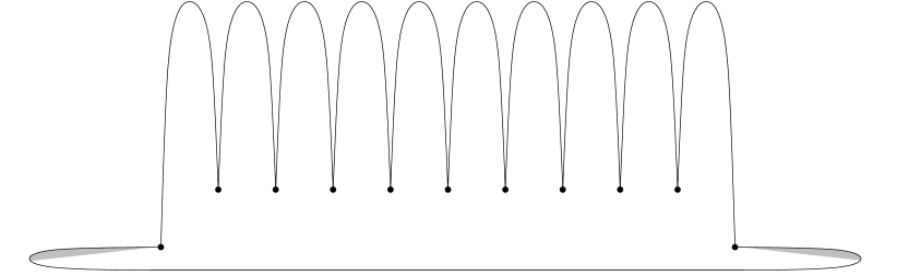
Figure 18: A monotone piecewise-convex polygon $M_{1}$ with an odd number of vertices that requires $\lfloor\frac{n}{2}\rfloor+1$ vertex guards in order to be guarded: the shaded regions require that at least one of the two endpoints of the bottom-most edge of the polygon to be in the guarding set.

\psfrag{r1}{\scriptsize$s_{1}$}\psfrag{r2}{\scriptsize$s_{2}$}\psfrag{r3}{\scriptsize$s_{3}$}\psfrag{r4}{\scriptsize$s_{4}$}\psfrag{r5}{\scriptsize$s_{5}$}\psfrag{x1}{\scriptsize$x_{1}$}\psfrag{x2}{\scriptsize$x_{2}$}\psfrag{x3}{\scriptsize$x_{3}$}\psfrag{x4}{\scriptsize$x_{4}$}\psfrag{x5}{\scriptsize$x_{5}$}\psfrag{x6}{\scriptsize$x_{6}$}\psfrag{x7}{\scriptsize$x_{7}$}\psfrag{x8}{\scriptsize$x_{8}$}\includegraphics[width=433.62pt]{fig/monotone_vertex_lb_even}

Figure 19: A monotone piecewise-convex polygon $M_{2}$ with an even number of vertices that requires $\lfloor\frac{n}{2}\rfloor+1$ vertex guards in order to be guarded.

The polygons $M_{1}$ and $M_{2}$ yielding the lower bound are shown in Figs. 18 and 19. $M_{1}$ has an odd number of vertices, whereas $M_{2}$ has an even number of vertices. Let $G_{1}$ (resp., $G_{2}$) be the vertex guarding set for $M_{1}$ (resp., $M_{2}$). Let us first consider $M_{1}$ (see Fig. 18). Notice that each prong of $M_{1}$ is fully guarded by either of its two endpoints; the other vertices of $M_{1}$ can only partially guard the prongs that they are not adjacent to. Moreover, the shaded regions of $M_{1}$ can only be guarded by $u_{1}$ or $u_{n}$. Suppose, now, we can guard $M_{1}$ with less than $\lfloor\frac{n}{2}\rfloor+1$ vertex guards. Then either two consecutive vertices $u_{i}$ and $u_{i+1}$ of $M_{1}$, $1\leq{}i\leq{}n-1$, will not belong to $G_{1}$, or $u_{1}$ and $u_{n}$ will not belong to $G_{1}$. In the former case, the prong that has $u_{i}$ and $u_{i+1}$ as endpoints is only partially guarded by the vertices in $G_{1}$, a contradiction. In the latter case, the shaded regions of $M_{1}$ are not guarded by the vertices in $G_{1}$, again a contradiction.

Consider now the polygon $M_{2}$ (see Fig. 19). The number of vertices of $M_{2}$ between $x_{1}$ and $x_{2}$ is equal to the number of vertices between $x_{7}$ and $x_{8}$, and even in number. Every prong of $M_{2}$ between $x_{1}$ and $x_{2}$ (resp., between $x_{7}$ and $x_{8}$) can be guarded by its two endpoints only; all other vertices of $M_{2}$ guard each such prong only partially. The shaded region $s_{1}$ (resp., $s_{5}$) is guarded only if either $x_{1}$ or $x_{3}$ (resp., either $x_{6}$ or $x_{8}$) belongs to $G_{2}$. The prong with endpoints $x_{2}$ and $x_{4}$ can be guarded by either both $x_{2}$ and $x_{4}$, or by $x_{3}$. If $x_{2}$ is the only vertex in $G_{2}$ among $x_{2}$, $x_{3}$ and $x_{4}$, then the shaded region $s_{4}$ is not guarded. Similarly, if $x_{4}$ is the only vertex in $G_{2}$ among $x_{2}$, $x_{3}$ and $x_{4}$, then the shaded region $s_{2}$ is not guarded. Finally, if neither $x_{4}$ nor $x_{5}$ belong to $G_{2}$, then the shaded prong $s_{3}$ is not guarded. Let us suppose now that $M_{2}$ can be guarded by less than $\lfloor\frac{n}{2}\rfloor+1$ vertex guards. By our observations above, it is not possible that two consecutive vertices $u_{i}$ and $u_{i+1}$ of $M_{2}$, $1\leq{}i\leq{}n-1$, do not belong to $G_{2}$. Hence $G_{2}$ will be a subset of the set $G_{2}^{\prime}=\{u_{2m-1},1\leq{}m\leq{}\lfloor\frac{n}{2}\rfloor\}$ or a subset of the set $G_{2}^{\prime\prime}=\{u_{2m},1\leq{}m\leq{}\lfloor\frac{n}{2}\rfloor\}$. In the former case, i.e., if $G_{2}\subseteq{}G_{2}^{\prime}$, neither $x_{6}$ nor $x_{8}$ belong to $G_{2}$, and thus the region $s_{5}$ is not guarded, a contradiction. Similarly, if $G_{2}\subseteq{}G_{2}^{\prime\prime}$, neither $x_{1}$ nor $x_{3}$ belong to $G_{2}$, and thus the region $s_{1}$ is not guarded, again a contradiction. We thus conclude that $|G_{2}|\geq{}\lfloor\frac{n}{2}\rfloor+1$.

Point guards.    We now turn our attention to guarding $P$ with point guards (refer again to Fig. 17). Define $G_{even}$ to be the vertex set $G_{even}=\{u_{2m},1\leq{}m\leq{}\lfloor\frac{n}{2}\rfloor\}$. If $u_{0}\neq{}u_{1}$, i.e., if $\kappa_{0}\neq\emptyset$, let $e_{f}$ be the first (left-most) edge of $P$, and $u_{\mu}$, $\mu>1$, the right-most endpoint of $e_{f}$ (the left-most endpoint of $e_{f}$ is necessarily $u_{1}$). If $u_{n+1}\neq{}u_{n}$, i.e., if $\kappa_{n+1}\neq\emptyset$, let $e_{l}$ be the last (right-most) edge of $P$, and $u_{\nu}$, $\nu<n$, the left-most endpoint of $e_{l}$ (the right-most endpoint of $e_{l}$ is necessarily $u_{n}$). Finally, let $u_{i}^{\prime}$, $2\leq{}i\leq{}n-1$ be the projection along $L^{\perp}$ of $u_{i}$ on the opposite monotone chain of $P$. Define the set $G$ according to the following procedure:

1. Set $G$ equal to $G_{even}$.

2. If $u_{0}\neq{}u_{1}$ and $\mu>2$, replace $u_{2}$ in $G$ by $u_{2}^{\prime}$.

3. If $u_{n+1}\neq{}u_{n}$ and $n$ is odd and $\nu<n-1$, replace $u_{2\lfloor\frac{n}{2}\rfloor}$ by $u_{2\lfloor\frac{n}{2}\rfloor}^{\prime}$.

As in the case of vertex guards, the set $G$ can be computed in linear time and space: $G_{even}$ can be computed in linear time and space, whereas determining if $u_{2}$ (resp., $u_{2\lfloor\frac{n}{2}\rfloor}$) is to be replaced in $G$ by $u_{2}^{\prime}$ (resp., $u_{2\lfloor\frac{n}{2}\rfloor}^{\prime}$) takes $O(1)$ time. The following lemma establishes that $G$ is indeed a point guarding set for $P$.

Lemma 13

The set $G$ defined according to the procedure above is a point guarding set for $P$.

Proof.  Every convex region $\kappa_{i}$, $3\leq{}i\leq{}n-3$ is guarded by either $u_{i}$ or $u_{i+1}$, since one of the two is in $G$.

Now consider the convex regions $\kappa_{0}$, $\kappa_{1}$ and $\kappa_{2}$. Both $u_{2}$ and $u_{2}^{\prime}$ lie on the common boundary of $\kappa_{1}$ and $\kappa_{2}$. Since either $u_{2}$ or $u_{2}^{\prime}$ is in $G$, we conclude that $\kappa_{1}$ and $\kappa_{2}$ are guarded. If $\kappa_{0}=\emptyset$, i.e., if $u_{0}\equiv{}u_{1}$, $\kappa_{0}$ is vacuously guarded. Suppose $\kappa_{0}\neq\emptyset$, i.e., $u_{0}\neq{}u_{1}$. Let $r_{f}$ be the room of $P$ corresponding to the edge $e_{f}$. Clearly, $\kappa_{0}\subseteq{}r_{f}$. We distinguish between the cases $\mu=2$ and $\mu>2$. If $\mu=2$, then $u_{2}\in{}G$ guards $r_{f}$ and thus $\kappa_{0}$. If $\mu>2$, the point $u_{2}^{\prime}\in{}G$ is a point on $e_{f}$. Therefore, $u_{2}^{\prime}$ guards $r_{f}$ and thus $\kappa_{0}$.

Finally, we consider the convex regions $\kappa_{n-2}$, $\kappa_{n-1}$ and $\kappa_{n}$. If $\kappa_{n}=\emptyset$, i.e., $u_{n+1}\equiv{}u_{n}$, $\kappa_{n}$ is vacuously guarded. Suppose, now, that $\kappa_{n}\neq\emptyset$, i.e., $u_{n+1}\neq{}u_{n}$. Let $r_{l}$ be the room of $P$ corresponding to the edge $e_{l}$. Clearly, $\kappa_{n}\subseteq{}r_{l}$. We distinguish between the cases “$n$ even” and “$n$ odd”. If $n$ is even, then both $u_{n-2}\equiv{}u_{2\lfloor\frac{n}{2}\rfloor-2}$ and $u_{n}\equiv{}u_{2\lfloor\frac{n}{2}\rfloor}$ belong to $G$. This immediately implies that all three $\kappa_{n-2}$, $\kappa_{n-1}$ and $\kappa_{n}$ are guarded: $\kappa_{n-2}$ is guarded by $u_{n-2}$, whereas $\kappa_{n-1}$ and $\kappa_{n}$ are guarded by $u_{n}$. If $n$ is odd, either $u_{n-1}\equiv{}u_{2\lfloor\frac{n}{2}\rfloor}$ or $u_{n-1}^{\prime}\equiv{}u_{2\lfloor\frac{n}{2}\rfloor}^{\prime}$ belongs to $G$. Since both $u_{n-1}$ and $u_{n-1}^{\prime}$ lie on the common boundary of $\kappa_{n-2}$ and $\kappa_{n-1}$, we conclude that both $\kappa_{n-2}$ and $\kappa_{n-1}$ are guarded. To prove that $\kappa_{n}$ is guarded, we further distinguish between the cases $\nu=n-1$ and $\nu<n-1$. If $\nu=n-1$, then $u_{n-1}\in{}G$ is an endpoint of $r_{l}$, and thus guards $\kappa_{n}$. If $\nu<n-1$, the point $u_{n-1}^{\prime}\in{}G$ is a point on $e_{l}$. Therefore, $u_{n-1}^{\prime}$ guards $r_{l}$ and thus $\kappa_{n}$. $\Box$

Figure 20: A comb-like monotone piecewise-convex polygon that requires $\lfloor\frac{n}{2}\rfloor$ point guards in order to be guarded: one point guard is required per prong.

As far as the minimum number of point guards required to guard a monotone piecewise-convex polygon is concerned, the polygon $M$, shown in Fig. 20, yields the sought for lower bound. Notice that is very similar to the well known comb-like linear polygon that establishes the lower bound on the number of point or vertex guards required to guard a linear polygon. In our case it is easy to see that we need at least one point guard per prong of the polygon, and since there are $\lfloor\frac{n}{2}\rfloor$ prongs we conclude that we need at least $\lfloor\frac{n}{2}\rfloor$ point guards in order to guard $M$.

We are now ready to state the following theorem that summarizes the results of this section.

Theorem 14

Given a monotone piecewise-convex polygon $P$ with $n\geq{}2$ vertices, $\lfloor\frac{n}{2}\rfloor+1$ vertex (resp., $\lfloor\frac{n}{2}\rfloor$ point) guards are always sufficient and sometimes necessary in order to guard $P$. Moreover, we can compute a vertex (resp., point) guarding set for $P$ of size $\lfloor\frac{n}{2}\rfloor+1$ (resp., $\lfloor\frac{n}{2}\rfloor$) in $O(n)$ time and $O(n)$ space.

5 Piecewise-concave polygons

In this section we deal with the problem of guarding piecewise-concave polygons using point guards. Guarding a piecewise-concave polygon with vertex guards may be impossible even for very simple configurations (see Fig. 22(a)). In particular we prove the following:

Theorem 15

Let $P$ be a piecewise-concave polygon with $n$ vertices. $2n-4$ point guards are always sufficient and sometimes necessary in order to guard $P$.

Proof.  To prove the sufficiency of $2n-4$ point guards we essentially apply the technique in [17] for illuminating disjoint compact convex sets — please refer to Fig. 21. We denote by $A_{i}$ the convex object delimited by $a_{i}$ and the chord $v_{i}v_{i+1}$ of $a_{i}$. Let $t_{i}(v_{j})$ be the tangent line to $a_{i}$ at $v_{j}$, $j=i,i+1$, and let $b_{i+1}$ be the bisecting ray of $t_{i}(v_{i+1})$, $t_{i+1}(v_{i+1})$ pointing towards the interior of $P$.

Construct a set of locally convex arcs $\mathcal{K}=\{\kappa_{1},\kappa_{2},\ldots,\kappa_{n}\}$ that lie entirely inside $P$ as such that (cf. [17]):

1. the endpoints of $\kappa_{i}$ are $v_{i}$, $v_{i+1}$,

2. $\kappa_{i}$ is tangent to $b_{i}$ (resp., $b_{i+1}$) at $v_{i}$ (resp., $v_{i+1}$),

3. if $S_{i}$ is the locally convex object defined by $\kappa_{i}$ and its chord $v_{i}v_{i+1}$, then $A_{i}\subseteq{}S_{i}$, $1\leq{}i\leq{}n$,

4. the arcs $\kappa_{i}$ are pairwise non-crossing, and

5. the number of tangencies between the elements of $\mathcal{K}$ is maximized.

Let $Q$ be the piecewise-concave polygon defined by the sequence of the arcs in $\mathcal{K}$.

\psfrag{v1}{\small$v_{1}$}\psfrag{v2}{\small$v_{2}$}\psfrag{v3}{\small$v_{3}$}\psfrag{v4}{\small$v_{4}$}\psfrag{v5}{\small$v_{5}$}\psfrag{v6}{\small$v_{6}$}\psfrag{v7}{\small$v_{7}$}\psfrag{v8}{\small$v_{8}$}\psfrag{v9}{\small$v_{9}$}\psfrag{v10}{\small$v_{10}$}\psfrag{v11}{\small$v_{11}$}\psfrag{r1}{{\color[rgb]{1,0,0}\small$u_{1}$}}\psfrag{r2}{{\color[rgb]{1,0,0}\small$u_{2}$}}\psfrag{r3}{{\color[rgb]{1,0,0}\small$u_{3}$}}\psfrag{r4}{{\color[rgb]{1,0,0}\small$u_{4}$}}\psfrag{r5}{{\color[rgb]{1,0,0}\small$u_{5}$}}\psfrag{r6}{{\color[rgb]{1,0,0}\small$u_{6}$}}\psfrag{r7}{{\color[rgb]{1,0,0}\small$u_{7}$}}\psfrag{r8}{{\color[rgb]{1,0,0}\small$u_{8}$}}\psfrag{r9}{{\color[rgb]{1,0,0}\small$u_{9}$}}\psfrag{r10}{{\color[rgb]{1,0,0}\small$u_{10}$}}\psfrag{r11}{{\color[rgb]{1,0,0}\small$u_{11}$}}\includegraphics[width=390.25534pt]{fig/piececoncaveub2}

Figure 21: The proof for the upper bound of Theorem 15. The polygon $P$ is shown with thick solid curvilinear arcs. The arcs $\kappa_{i}$ are shown as thin solid arcs. The dotted rays are the bisecting rays $b_{i}$, whereas the dashed ray is the ray $r_{8}(v_{9})$. The regions $A_{8}$, $S_{8}\setminus{}A_{8}$ and $\Pi_{8}\setminus{}S_{8}$ are also shown using three levels of gray; note that $\Pi_{8}$ has one reflex vertex at $v_{9}$. The graph $\Gamma$ (i.e., the triangulation graph $\mathcal{T}({R})$) is shown in red: the node $u_{i}$ corresponds to the arc $a_{i}$ and the polygon $R$ is depicted via thick segments.

Suppose now that $\kappa_{i}$ and $\kappa_{\sigma(j)}$ are tangent, $1\leq{}j\leq{}m$, and let $\ell_{i,\sigma(j)}$ be the common tangent to $\kappa_{i}$ and $\kappa_{\sigma(j)}$. Let $s_{i,\sigma(j)}$ be the line segment on $\ell_{i,\sigma(j)}$ between the points of intersection of $\ell_{i,\sigma(j)}$ with $\ell_{i,\sigma(j-1)}$ and $\ell_{i,\sigma(j+1)}$. Let $\Pi_{i}$ be the polygonal region defined by the chord $v_{i}v_{i+1}$ and the line segments $s_{i,\sigma(j)}$. $\Pi_{i}$ is a linear polygon with at most two reflex vertices (at $v_{i}$ and/or $v_{i+1}$). It is easy to see that placing guards on the vertices of the $\Pi_{i}$’s guards both $P$ and $Q$. Let $G_{Q}$ be the guard set of $P$ constructed this way. Construct, now, a planar graph $\Gamma$ with vertex set $\mathcal{K}$. Two vertices $\kappa_{i}$ and $\kappa_{j}$ of $\Gamma$ are connected via an edge if $\kappa_{i}$ and $\kappa_{j}$ are tangent. The graph $\Gamma$ is a planar graph combinatorially equivalent to the triangulation graph $\mathcal{T}({R})$ of a polygon $R$ with $n$ vertices. The edges of $\Gamma$ connecting the arcs $\kappa_{i}$, $\kappa_{i+1}$, $1\leq{}i\leq{}n$, are the boundary edges of $R$, whereas all other edges of $\Gamma$ correspond to diagonals in $\mathcal{T}({R})$. Let ${{Q}^{\circ}}$ denote the interior of $Q$. Observing that ${{Q}^{\circ}}$ consists of a number of faces that are in 1–1 correspondence with the triangles in $\mathcal{T}({R})$, we conclude that ${{Q}^{\circ}}$ consists of $n-2$ faces, each containing three guards of $G_{Q}$. It fact, each face of ${{Q}^{\circ}}$ can actually be guarded by only two of the three guards it contains and thus we can eliminate one of them per face of ${{Q}^{\circ}}$. The new guard set $G$ of $Q$ constructed above is also a guard set for $P$ and contains $2(n-2)$ point guards.

To prove the necessity, refer to the piecewise-concave polygon $P$ in Fig. 22(b). Each one of the pseudo-triangular regions in the interior of $P$ requires exactly two point guards in order to be guarded. Consider for example the pseudo-triangle $\tau$ shown in gray in Fig. 22(b). We need one point along each one of the lines $l_{1}$, $l_{2}$ and $l_{3}$ in order to guard the regions near the corners of $\tau$, which implies that we need at least two points in order to guard $\tau$ (two out of the three points of intersection of the lines $l_{1}$, $l_{2}$ and $l_{3}$). The number of such pseudo-triangular regions is exactly $n-2$, thus we need a total of $2n-4$ point guards to guard $P$. $\Box$

(a)

\psfrag{l1}{\small$l_{1}$}\psfrag{l2}{\small$l_{2}$}\psfrag{l3}{\small$l_{3}$}\includegraphics[width=325.215pt]{fig/concavelb}

(b)

Figure 22: (a) A piecewise-concave polygon $P$ that cannot be guarded solely by vertex guards. Two consecutive edges of $P$ have a common tangent at the common vertex and as a result the three vertices of $P$ see only the points along the dashed segments. (b) A piecewise-concave polygon $P$ that requires $2n-4$ point guards in order to be guarded.

6 Locally convex and general polygons

We have so far been dealing with the cases of piecewise-convex and piecewise-concave polygons. In this section we will present results about locally convex, monotone locally convex and general polygons.

Locally convex polygons.    The situation for locally convex polygons is much less interesting, as compared to piecewise-convex polygons, in the sense that there exist locally convex polygons that require $n$ vertex guards in order to be guarded. Consider for example the locally convex polygon of Fig. 23(a). Every room in this polygon cannot be guarded by a single guard, but rather it requires both vertices of every locally convex edge to be in any guarding set in order for the corresponding room to be guarded. As a result it requires $n$ vertex guards. Clearly, these $n$ guards are also sufficient, since any one of them guards also the central convex part of the polygon. More interestingly, even if we do not restrict ourselves to vertex guards, but rather allow guards to be any point in the interior or the boundary of the polygon, then the locally convex polygon in Fig. 23(a) still requires $n$ guards. This stems from the fact that the rooms of this polygon have been constructed in such a way so that the kernel of each room is the empty set (i.e., they are not star-shaped objects). However, we can guard each room with two guards, which can actually be chosen to be the endpoints of the locally convex arcs.

\psfrag{v1}{$v_{1}$}\psfrag{v2}{$v_{2}$}\psfrag{a1}{$a_{1}$}\psfrag{a2}{$a_{2}$}\psfrag{l}{$\ell$}\includegraphics[width=130.08731pt]{fig/locallyconvexall}

(a)

\psfrag{v1}{$v_{1}$}\psfrag{v2}{$v_{2}$}\psfrag{a1}{$a_{1}$}\psfrag{a2}{$a_{2}$}\psfrag{l}{$\ell$}\includegraphics[width=130.08731pt]{fig/nonconvexinfinite}

(b)

Figure 23: (a) A locally convex polygon with $n$ vertices that requires $n$ vertex or point guards in order to be guarded. (b) A non-convex polygon that cannot be guarded by vertex guards, and which requires an infinite number of point guards.

In fact the $n$ vertices of a locally convex polygon are not only necessary (in the worst case), but also always sufficient. Consider a point $q$ inside a locally convex polygon $P$ and let $\rho_{q}$ be an arbitrary ray emanating from $q$. Let $w_{q}$ be the first point of intersection of $\rho_{q}$ with the boundary of $P$ as we walk on $\rho_{q}$ away from $q$. If $w_{q}$ is a vertex of $P$ we are done: $q$ is visible by one of the vertices of $P$. Otherwise, rotate $\rho_{q}$ around $q$ in the, say, counterclockwise direction, until the line segment $qw_{q}$ hits a feature $f$ of $P$ (if multiple features of $P$ are hit at the same time, consider the one closest to $q$ along $\rho_{q}$). $f$ cannot be a point in the interior of an edge of $P$ since then $P$ would have to be locally concave at $f$. Therefore, $f$ has to be a vertex of $P$, i.e., $q$ is guarded by $f$. We can thus state the following theorem:

Theorem 16

Let $P$ be a locally convex polygon with $n\geq{}2$ vertices. Then $n$ vertex (the $n$ vertices of $P$) or point guards are always sufficient and sometimes necessary in order to guard $P$.

Monotone locally convex polygons.    As far as monotone locally convex polygons are concerned, it easy to see that $\lfloor\frac{n}{2}\rfloor+1$ vertex or point guards are always sufficient. Let $P$ be a locally convex polygon. As in the case of piecewise-convex polygons, assume without loss of generality that $P$ is monotone with respect to the $x$-axis. Let $u_{1},\ldots,u_{n}$ be the vertices of $P$ sorted with respect to their $x$-coordinate. To prove our sufficiency result, it suffices to consider the vertical decomposition of $P$ into at most $n+1$ convex regions $\kappa_{i}$, $0\leq{}i\leq{}n$. Corollary 12 remains valid. As a result, the vertex set $G=\{u_{2m-1},1\leq{}m\leq{}\lfloor\frac{n}{2}\rfloor\}\cup\{u_{n}\}$ is a guarding set for $P$ of size $\lfloor\frac{n}{2}\rfloor+1$: every convex region $\kappa_{i}$, $1\leq{}i\leq{}n-1$ is guarded by either $u_{i}$ or $u_{i+1}$, since at least one of $u_{i}$, $u_{i+1}$ is in $G$; moreover, $u_{1}$ and $u_{n}$ guard $\kappa_{0}$ and $\kappa_{n}$, respectively. As in the case of piecewise-convex polygons, $G$ can be computed in linear time and space.

In fact, the upper bound on the number of vertex/point guards for $P$ just presented is also a worst case lower bound. Consider the locally convex polygons $T_{1}$ and $T_{2}$ of Fig. 24, each consisting of $n$ vertices. $T_{1}$ has an odd number of vertices, while the number of vertices of $T_{2}$ is even. It is readily seen that both $T_{1}$ and $T_{2}$ need at least one point guard per prong (including the right-most prong of $T_{1}$ and both the left-most and right-most prongs of $T_{2}$). Since the number of prongs in either $T_{1}$ or $T_{2}$ is $\lfloor\frac{n}{2}\rfloor+1$, we conclude that $T_{1}$ and $T_{2}$ require at least $\lfloor\frac{n}{2}\rfloor+1$ point guards in order to be guarded. Summarizing our results about monotone locally convex polygons:

Theorem 17

Given a monotone locally convex polygon $P$ with $n\geq{}2$ vertices, $\lfloor\frac{n}{2}\rfloor+1$ vertex or point guards are always sufficient and sometimes necessary in order to guard $P$. Moreover, we can compute a vertex guarding set for $P$ of size $\lfloor\frac{n}{2}\rfloor+1$ in $O(n)$ time and $O(n)$ space.

Figure 24: Two comb-like monotone locally convex polygons $T_{1}$ (top) and $T_{2}$ (bottom) with an odd and even number of vertices, respectively. Both polygons require $\lfloor\frac{n}{2}\rfloor+1$ point guards in order to be guarded: one point guard is required per prong.

Remark 3

The results presented in this section about locally convex polygons are in essence the same with known results on the number of reflex vertices required to guard linear polygons. In particular, it is known that if a linear polygon $P$ has $r\geq{}1$ reflex vertices, $r$ vertex guards placed on these vertices are always sufficient and sometimes necessary in order to guard $P$ [28], whereas if $P$ is a monotone linear polygon, $\lfloor\frac{r}{2}\rfloor+1$ among its $r$ reflex vertices are always sufficient and sometimes necessary in order to guard $P$ [1]. In our setting, the $r$ reflex vertices of the linear polygon $P$ are the $n$ vertices of our locally convex polygons, and the locally convex polylines connecting the reflex vertices of $P$ are our locally convex edges. Clearly, the analogy only refers to the combinatorial complexity of guarding sets, since for our algorithmic analysis we have assumed that the polygon edges have constant complexity.

In the context we have just described, i.e., seeing linear polygons as locally convex polygons the vertices of which are the reflex vertices of the linear polygons, it also possible to “translate” the results of Section 3 as follows:

Consider a linear polygon $P$ with $r\geq{}2$ reflex vertices. If $P$ can be decomposed into $c\geq{}r$ convex polylines pointing towards the exterior of the polygon, then $P$ can be guarded with at most $\lfloor\frac{2c}{3}\rfloor$ vertex guards.

The analogous “translation” for the results of Section 5 is as follows:

Consider a linear polygon $P$ with $n$ vertices, $r$ of which are reflex. If $P$ can be decomposed into $c\geq{}n-r$ convex polylines pointing towards the interior of the polygon, then $P$ can be guarded with at most $2c-4$ point guards.

General polygons.    The class of general polygons poses difficulties. Consider the non-convex polygon $N$ of Fig. 23(b), which consists of two vertices $v_{1}$ and $v_{2}$ and two convex arcs $a_{1}$ and $a_{2}$. The two arcs are tangent to a common line $\ell$ at $v_{1}$. It is readily visible that $v_{1}$ and $v_{2}$ cannot guard the interior of $N$. In fact, $v_{1}$ cannot guard any point of $N$ other than itself. Even worse, any finite number of guards, placed anywhere in $N$, cannot guard the polygon. To see that, consider the vicinity of $v_{1}$. Assume that $N$ can be guarded by a finite number of guards, and let $g\neq v_{1}$ be the guard closest to $v_{1}$ with respect to shortest paths within $N$. Consider the line $\ell_{g}$ passing through $g$ that is tangent to $a_{2}$ (among the two possible tangents we are interested in the one the point of tangency of which is closer to $v_{1}$). Let $s_{g}$ be the sector of $N$ delimited by $a_{1}$, $a_{2}$ and $\ell_{g}$. $s_{g}$ cannot contain any guarding point, since such a vertex would be closer to $v_{1}$ than $g$. Since $s_{g}$ is not guarded by $v_{1}$, we conclude that $s_{g}$ is not guarded at all, which contradicts our assumption that $N$ is guarded by a finite set of guards.

7 Summary and future work

In this paper we have considered the problem of guarding a polygonal art gallery, the walls of which are allowed to be arcs of curves (our results are summarized in Table 1). We have demonstrated that if we allow these arcs to be locally convex arcs, $n$ (vertex or point) guards are always sufficient and sometimes necessary. If these arcs are allowed to be non-convex, then an infinite number of guards may be required. In the case of piecewise-convex polygons with $n$ vertices, we have shown that it is always possible to guard the polygon with $\lfloor\frac{2n}{3}\rfloor$ vertex guards, whereas $\lfloor\frac{4n}{7}\rfloor-1$ vertex guards are sometimes necessary. Furthermore, we have described an $O(n\log n)$ time and $O(n)$ space algorithm for computing a vertex guarding set of size at most $\lfloor\frac{2n}{3}\rfloor$. For piecewise-concave polygons, we have shown that $2n-4$ point guards are always sufficient and sometimes necessary. Finally, in the special case of monotone piecewise-convex polygons, $\lfloor\frac{n}{2}\rfloor+1$ vertex or $\lfloor\frac{n}{2}\rfloor$ point guards are always sufficient and sometimes necessary, whereas for monotone locally convex polygons $\lfloor\frac{n}{2}\rfloor+1$ vertex or point guards are always sufficient and sometimes necessary.

Up to now we have not found a piecewise-convex polygon that requires more than $\lfloor\frac{4n}{7}\rfloor+O(1)$ vertex guards, nor have we devised a polynomial time algorithm for guarding a piecewise-convex polygon with less than $\lfloor\frac{2n}{3}\rfloor$ vertex guards. Closing the gap between then two complexities remains an open problem. Another open problem is the worst case maximum number of point guards required to guard a piecewise-convex polygon. In this case our lower bound construction fails, since it is possible to guard the corresponding polygon with $\lfloor\frac{3n}{7}\rfloor+O(1)$ point guards. On the other hand, the comb-like polygon shown in Fig. 20, requires $\lfloor\frac{n}{2}\rfloor$ point guards. Clearly, our algorithm that computes a guarding set of at most $\lfloor\frac{2n}{3}\rfloor$ vertex guards is still applicable.

	Bounds by guard type
Polygon type	Vertex		Point
	Upper	Lower	Upper	Lower
Piecewise-convex	$\lfloor\frac{2n}{3}\rfloor$	$\lfloor\frac{4n}{7}\rfloor-1$	$\lfloor\frac{2n}{3}\rfloor$	$\lfloor\frac{n}{2}\rfloor$
Monotone piecewise-convex	$\lfloor\frac{n}{2}\rfloor+1$		$\lfloor\frac{n}{2}\rfloor$
Locally convex	$n$
Monotone locally convex	$\lfloor\frac{n}{2}\rfloor+1$
Piecewise-concave	not always possible		$2n-4$
General	not always possible		$\infty$

Table 1: The results in this paper: worst case upper and lower bounds on the number of vertex or point guards needed in order to guard different types of curvilinear polygons.

Other types of guarding problems have been studied in the literature, which either differ on the type of guards (e.g., edge or mobile guards), the topology of the polygons considered (e.g., polygons with holes) or the guarding model (e.g., the fortress problem or the prison yard problem, mentioned in Section 1); see the book by O’Rourke [28], the survey paper by Shermer [30] of the book chapter by Urrutia [33] for an extensive list of the variations of the art gallery problem with respect to the types of guards or the guarding model. It would be interesting to extend these results to the families of curvilinear polygons presented in this paper.

Last but not least, in the case of general polygons, is it possible to devise an algorithm for computing a guarding set of finite cardinality, if the polygon does not contain cusp-like configurations such as the one in Fig. 23(b)?

References

[1]
A. Aggarwal.
The art gallery problem: Its variations, applications, and
algorithmic aspects.
PhD thesis, Dept. of Comput. Sci., Johns Hopkins University,
Baltimore, MD, 1984.
[2]
D. Avis and H. ElGindy.
A combinatorial approach to polygon similarity.
IEEE Trans. Inform. Theory, IT-2:148–150, 1983.
[3]
J.-D. Boissonnat and M. Teillaud, editors.
Effective Computational Geometry for Curves and Surfaces.
Mathematics and Visualization. Springer, 2007.
[4]
W. Bronsvoort.
Boundary evaluation and direct display of CSG models.
Computer-Aided Design, 20:416–419, 1988.
[5]
B. Chazelle.
Triangulating a simple polygon in linear time.
In Proc. 31st Annu. IEEE Sympos. Found. Comput. Sci., pages
220–230, 1990.
[6]
B. Chazelle.
Triangulating a simple polygon in linear time.
Discrete Comput. Geom., 6(5):485–524, 1991.
[7]
B. Chazelle and J. Incerpi.
Triangulation and shape-complexity.
ACM Trans. Graph., 3(2):135–152, 1984.
[8]
V. Chvátal.
A combinatorial theorem in plane geometry.
J. Combin. Theory Ser. B, 18:39–41, 1975.
[9]
C. Coullard, B. Gamble, W. Lenhart, W. Pulleyblank, and G. Toussaint.
On illuminating a set of disks.
Manuscript, 1989.
[10]
J. Czyzowicz, B. Gaujal, E. Rivera-Campo, J. Urrutia, and J. Zaks.
Illuminating higher-dimensionall convex sets.
Geometriae Dedicata, 56:115–120, 1995.
[11]
J. Czyzowicz, E. Rivera-Campo, J. Urrutia, and J. Zaks.
Protecting convex sets.
Graphs and Combinatorics, 19:311–312, 1994.
[12]
M. de Berg, M. van Kreveld, M. Overmars, and O. Schwarzkopf.
Computational Geometry: Algorithms and Applications.
Springer-Verlag, Berlin, Germany, 2nd edition, 2000.
[13]
D. P. Dobkin and D. L. Souvaine.
Computational geometry in a curved world.
Algorithmica, 5:421–457, 1990.
[14]
H. Edelsbrunner, J. O’Rourke, and E. Welzl.
Stationing guards in rectilinear art galleries.
Comput. Vision Graph. Image Process., 27:167–176, 1984.
[15]
K. Eo and C. Kyung.
Hybrid shadow testing scheme for ray tracing.
Computer-Aided Design, 21:38–48, 1989.
[16]
D. Eppstein, M. T. Goodrich, and N. Sitchinava.
Guard placement for efficient point-in-polygon proofs.
In Proc. 23rd Annu. ACM Sympos. Comput. Geom., pages 27–36,
2007.
[17]
L. Fejes Tóth.
Illumination of convex discs.
Acta Math. Acad. Sci. Hungar., 29(3–4):355–360, 1977.
[18]
S. Fisk.
A short proof of Chvátal’s watchman theorem.
J. Combin. Theory Ser. B, 24:374, 1978.
[19]
J. Kahn, M. M. Klawe, and D. Kleitman.
Traditional galleries require fewer watchmen.
SIAM J. Algebraic Discrete Methods, 4:194–206, 1983.
[20]
R. Kuc and M. Siegel.
Efficient representation of reflecting structures for a sonar
navigation model.
In Proc. 1987 IEEE Int. Conf. Robotics and Automation, pages
1916–1923, 1987.
[21]
D. Lee and A. Lin.
Computational complexity of art gallery problems.
IEEE Trans. Inform. Theory, 32(2):276–282, 1986.
[22]
D. T. Lee and F. P. Preparata.
Location of a point in a planar subdivision and its applications.
SIAM J. Comput., 6(3):594–606, 1977.
[23]
T. Lozano-Pérez and M. A. Wesley.
An algorithm for planning collision-free paths among polyhedral
obstacles.
Commun. ACM, 22(10):560–570, 1979.
[24]
A. Lubiw.
Decomposing polygonal regions into convex quadrilaterals.
In Proc. 1st Annu. ACM Sympos. Comput. Geom., pages 97–106,
1985.
[26]
G. Meisters.
Polygons have ears.
Amer. Math. Monthly, 82:648–651, 1975.
[27]
J. S. B. Mitchell.
An algorithmic approach to some problems in terrain navigation.
In D. Kapur and J. Mundy, editors, Geometric Reasoning. MIT
Press, Cambridge, MA, 1989.
[28]
J. O’Rourke.
Art Gallery Theorems and Algorithms.
The International Series of Monographs on Computer Science. Oxford
University Press, New York, NY, 1987.
[29]
J.-R. Sack.
Rectilinear computational geometry.
Ph.D. thesis, School Comput. Sci., Carleton Univ., Ottawa, ON,
1984.
Report SCS-TR-54.
[30]
T. C. Shermer.
Recent results in art galleries.
Proc. IEEE, 80(9):1384–1399, Sept. 1992.
[31]
J. Stenstrom and C. Connolly.
Building wire frames for multiple range views.
In Proc. 1986 IEEE Conf. Robotics and Automation, pages
615–650, 1986.
[32]
G. T. Toussaint.
Pattern recognition and geometrical complexity.
In Proc. 5th IEEE Internat. Conf. Pattern Recogn., pages
1324–1347, 1980.
[33]
J. Urrutia.
Art gallery and illumination problems.
In J.-R. Sack and J. Urrutia, editors, Handbook of Computational
Geometry, pages 973–1027. North-Holland, 2000.
[34]
J. Urrutia and J. Zaks.
Illuminating convex sets.
Technical Report TR-89-31, Dept. Comput. Sci., Univ. Ottawa,
Ottawa, ON, 1989.
[35]
S. Xie, T. Calvert, and B. Bhattacharya.
Planning views for the incremental construction of body models.
In Proc. Int. Conf. Pattern Recongition, pages 154–157, 1986.
[36]
M. Yachida.
3-D data acquisition by multiple views.
In Robotics Research: Third Int. Symp., pages 11–18, 1986.